Ensemble learning landslide susceptibility assessment with optimized non-landslide samples selection

Abstract

Non-landslide samples influence the outcomes of landslide susceptibility assessment. Existing studies did not fully consider the equilibrium between landslide and non-landslide samples in similar environments, resulting in poor reliability of landslide susceptibility assessment. This study proposed a non-landslide samples optimization method with a constraint of disaster-pregnant environment similarity to construct the balanced landslide and non-landslide samples. We employed the heterogeneous stacking and blending ensemble learning models to generate the landslide susceptibility assessment. This study focused on the Bailong River Basin with complex environment and frequent landslides as the study area. First, we extracted 12 landslide influencing factors based on multiple sources and analyzed the spatial distribution patterns of landslides. Second, we constructed similar environments based on the assessment units obtained from the curvature watershed method and selected an equal amount of both landslide and non-landslide samples in every different environment. Finally, three classic neural network models, namely multilayer perceptron, convolutional neural network, and gated recurrent unit were used as base models for stacking and blending ensemble learning models to assess landslide susceptibility. The findings suggested that the landslide susceptibility assessment results with optimized non-landslide samples were more reliable, especially the proposed method improved the prediction results in sample-sparse regions. The stacking ensemble constructed in this study demonstrated the highest area under the curve of 0.88 for the testing dataset, outperforming the blending ensemble and three base models. The issue of unreliable landslide susceptibility assessment results in sample-sparse regions within complex environments can be effectively addressed by considering the balanced sampling of non-landslide samples under the constraint of similar environments.

Keywords:

• Landslide susceptibility
• ensemble learning
• similar environments
• non-landslide samples selection

1. Introduction

Landslides represent an extremely destructive natural geological phenomenon that is prevalent in mountainous regions of China. They seriously endanger people’s lives, disrupt normal production and daily life, and result in significant losses to the national economy (Dai, Li, et al. 2023; Chen, Gao, et al. 2024). Early identification and prevention of landslides are crucial measures for mitigating and preventing disaster-related losses. Landslide susceptibility assessment can investigate the intricate connection between landslides and environments by selecting models and data. Landslide susceptibility assessment can comprehensively assess the likelihood of unclear landslides occurring in similar environments, serving as an effective visualization technique for localizing landslide areas and managing land resources sustainably (Ma et al. 2021; Dai, Chen, et al. 2023). Additionally, landslide susceptibility assessment offers robust technical support for decision-making managers (Chang et al. 2020).

Landslide susceptibility assessment methods can generally be categorized into model-driven and data-driven. Model-driven methods involve mechanistic mechanisms and rules of thumb. Data-driven methods encompass statistical regression and machine learning (Zhu et al. 2019). Compared to other methods, machine learning methods demonstrate strong capabilities in processing nonlinear relationships and possesses robust self-learning abilities, which enable the extraction of potential feature correlations (Huang et al. 2020). Machine learning can be divided into traditional machine learning and deep learning. Traditional machine learning has gradually gained widespread application in landslide susceptibility assessment, such as support vector machines (Huang and Zhao 2018) and decision tree models including random forests (RF) (Chen et al. 2017), Extreme Gradient Boosting (XGBoost), and Light Gradient Boosting Machine (LightGBM) (Zeng, Jin, et al. 2024). With the continuous advancement of technology, deep learning models have shown outstanding performance in landslide susceptibility assessment (Dou et al. 2020; Chen, Wang, et al. 2024), such as convolutional neural network (CNN) (Wang et al. 2019) and Long Short-Term Memory (Zeng, Glade, et al. 2023). Compared with traditional machine learning methods, the deep learning model is processed layer by layer, and the original data features can be deeply extracted. Therefore, the ability to solve complex nonlinear is stronger, and the accuracy is higher when processing large sample data (Achu, Aju, et al. 2023; Zeng, Wu, et al. 2024). Deep learning has different focuses on capturing various features, which makes it prone to local optima and challenging to apply universally to all case scenarios (Merghadi et al. 2018). In a large-scale, complex, and heterogeneous geographical environments, single deep learning model can lead to poor reliability in landslide susceptibility assessment. Scholars have adopted heterogeneous ensemble strategies, extracting features from various data perspectives to address the constraints of individual models, optimize model performance, and significantly improve assessment accuracy and generalization capabilities (Wang et al. 2020; He, Zhao, et al. 2021; Lv et al. 2022; Zhao et al. 2024), such as stacking and blending ensembles (Fang et al. 2021; Zeng, Guo, et al. 2023). Zeng, Wu, et al. (2024) used Stacking to integrate RF and XGboost to obtain primary landslide susceptibility assessment, which combined with multi-temporal interferometric SAR for enhanced landslide susceptibility assessment. However, landslide susceptibility modelling relies heavily on the creation of a robust dataset.

The number of landslide samples has a great influence on the performance of deep learning (Achu, Thomas, et al. 2023). However, in complex scenarios, especially in high-altitude and densely vegetated areas, there may be no labelled samples or an insufficient number of labelled samples, which exacerbates the imbalance between landslide and non-landslide samples (Li et al. 2018; Du et al. 2020; Zhang et al. 2024). To get the balance data, there are a variety of the non-landslide sample selection method. Traditional random sampling methods involve the random selection of non-landslide samples from outside the known landslide zones (Zhou et al. 2018). This method neglects disaster-pregnant environmental characteristics that are conducive to landslide occurrence. This oversight prevents machine learning models from thoroughly exploring potential correlations in landslide features. In addition, the methods of randomly selecting non-landslide samples from initial zones with very low susceptibility (Huang et al. 2021) and non-landslide zones with slopes below or above a specific threshold (Trinh et al. 2023) are also commonly used for landslide susceptibility prediction. However, these methods have limitations that do not comprehensively represent the overall characteristics of non-landslide samples. Existing methods cannot synthesize the influence of the environment on landslides when selecting non-landslide samples. Ensuring the representativeness and balance of the collected non-landslide samples is challenging, which can lead to unbalanced prediction effects in complex environments, thereby causing elevated rates of false alarms and miss. Models trained with limited and unbalanced labelled samples inevitably result in overfitting. Especially when the samples contain noise, it may even lead to the training of incorrect models (Zhu et al. 2020), which seriously affects the reliability of machine learning methods for assessing landslide susceptibility. Accurately selecting representative and balanced non-landslide samples remains a crucial challenge in machine learning models for assessing landslide susceptibility.

In response to the challenges posed by various non-landslide sample selection methods that fail to comprehensively consider the environmental impact on landslides, resulting in imbalanced effects in complex environments, we proposed an optimized method that uses a constraint of similar environments to select non-landslide samples. This method aims to enhance the representativeness and balance of non-landslide samples, thereby addressing the unreliable susceptibility results in sparsely sampled regions within complex environments. We selected the Bailong River Basin with complex environment and frequent landslides as the study area. We selected lithology, soil type, distance to rivers, and distance to faults as disaster-pregnant environmental factors to delineate similar environments based on slope units and selected non-landslide samples using similarity constraints. We applied stacking and blending heterogeneous ensemble learning models for the landslide susceptibility mapping (LSM) based on multilayer perceptron (MLP), CNN, and gated recurrent unit (GRU) three deep learning models.

2. Study area and data

2.1. Study area

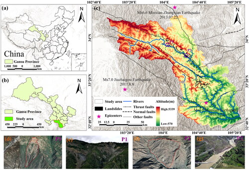
The Bailong River Basin is located in southern Gansu Province and covers an area of over 20,000 km² (Figure 1). Average annual precipitation in the southern region experiences an average annual precipitation of 450–800 mm, while the northern part is 400–700 mm. The study area is typical mountainous terrain, with significant topographic undulations and a complex geographic environment. Influenced by factors such as tectonic movements, concentrated rainfall, and human activities, the region is prone to frequent and widespread geological disasters. As a result, it is considered one of the four major high-risk areas for landslides and debris flows in China. The Wenchuan earthquake, with a magnitude of 8.0, on May 12, 2008, exacerbated the damage to mountains and geotechnical structures. It triggered a series of new landslides and mudslides and caused a large number of concealed geohazards. Subsequent earthquakes, such as the 6.6-magnitude earthquakes in Min County and Zhang County in 2013, the 4.5-magnitude earthquake in Wen County in 2013, and the 7.0-magnitude earthquake in Jiuzhaigou County in 2017, further contributed to the deformation and fragmentation of rock-soil formations. These seismic events provided favourable pathways for surface infiltration and groundwater activities, creating conducive material and structural conditions for the formation, development, and occurrence of landslides. Landslide hazards in the Bailong River Basin not only pose a serious threat to the lives and property of the local residents and vital infrastructure but also jeopardize the ecological security and sustainable development of the region and even the upstream region of the Yangtze River.

Figure 1. Study area and historical landslide distribution:(a) Gansu in China, (b)study area in Gansu province, (c) historical landslides, (d) the google image and landslide boundary of North Hill landslide, (e) the field photograph of North Hill landslide, (f) the google image and landslide boundary of Jiangdingya landslide, (g) the field photograph of Jiangdingya landslide.

2.2. Historical landslide dataset

Accurate identification of historical landslides is crucial for landslide susceptibility assessment (Wei et al. 2022). The landslide inventory was obtained through field investigation, interpretation of Google Earth imagery, and compilation of historical records, as illustrated in Figure 1(c). Moreover, Figure 1(d) displays the vector of the Beishan landslide in Lijie township, Zhouqu County, on January 18, 2021, interpreted from Google image, with corresponding field photograph shown in Figure 1(e). Similarly, Figure 1(f) shows the vector of Jiangdingya landslide that occurred in Nanyu township, Zhouqu County, on July 12, 2018, with corresponding field photograph shown in Figure 1(g). The landslide inventory has a total of 638 landslides, with the largest landslide covering an area of 4.48 km². These landslides are mainly loess landslides, debris landslides, and fractured rock landslides. They are typically triggered by seasonal rainfall and seismic activity, primarily distributed along both sides of rivers and valleys. Over 90% of landslides in the basin are concentrated within a distance of less than 4000 m from faults. There is a clear concentration of landslides at fault intersections and offsets. Furthermore, conducting landslide samples in remote, densely vegetated, and high-altitude areas presents challenges, resulting in limited landslide data.

2.3. Landslide influencing factors

Selecting the appropriate landslide influencing factors (LIFs) is a crucial step in landslide susceptibility modelling. Considering the evolution and characteristics of landslides, relevant research findings, and the specific features of the study area, 12 LIFs were selected. These factors include elevation, slope, profile curvature, terrain wetness index (TWI), rainfall, land use, normalized vegetation index (NDVI), lithology, soil type, distance to roads, distance to rivers, and distance to faults (Figure 2). The data sources are specified in Table 1. Historical landslides are primarily concentrated within proximity both faults and rivers, which jointly influence the occurrence of landslides. Therefore, they are considered as important disaster-pregnant environmental factors. Soil type and lithology exhibit a strong correlation in spatial distribution with the distance to faults and rivers. Moreover, the types of historical landslides also demonstrate distinct geological characteristics, they are also considered as disaster-pregnant environmental factors. These factors serve as the basis for subsequent environmental delineation to constrain the impact of different environments on landslide development. Due to variations in the resolution of different datasets, the collected landslide disaster factors had different scales. For the purpose of simplifying subsequent feature extraction, all LIFs were uniformly resampled to 30 × 30 m resolution.

Figure 2. The spatial distribution of LIFs: (a) altitude, (b) slope, (c) profile curvature, (d) TWI, (e) rainfall, (f) land use, (g) NDVI, (h) lithology, (i) soil type, (j) distance to roads, (k) distance to Rivers, (l) distance to faults.

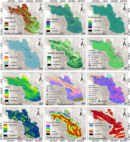
Table 1. The sources of data for LIFs used in this study.

Data name	Data source	Type	Resolution	LIFs
DEM	https://vertex.daac.asf.alaska.edu	Raster	12.5m	Altitude
				Slope
				Profile curvature
				TWI
Land use	http://globallandcover.com/	Raster	30m	Land use
River	https://www.openhistori calmap.org	Vector	1:5000	Distance to rivers
Vegetation normalization index	http://www.geodata.cn/	Raster	1000m	NDVI
Soil type	http://www.fao.org/soils-portal	Raster	1000m	Soil type
Geological map	http://geodb.cgs.gov.cn/	Vector	1:1,000,000	Lithology
				Distance to faults
Road	http://data.tpdc.ac.cn	Vector	1:1,000,000	Distance to roads
Rainfall	http://www.geodata.cn/	Raster	1000m	Annual average cumulative rainfall

3. Methods

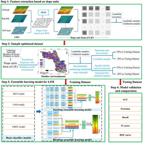
The technical workflow of this study is illustrated in Figure 3. First, the new form of LIFs is obtained by extracting LIFs using slope units, and they are categorized as landslide samples and unlabelled samples based on the landslide inventory. Second, the dataset is constructed using a balanced sampling strategy of the disaster-pregnant environment similarity to enhance the representativeness and balance of the non-landslide samples. A total of 70% of the dataset is allocated to train model, while the remaining 30% is allocated to test model. Third, ensemble models were constructed based on MLP, CNN, and GRU methods to generate landslide susceptibility assessment. Ultimately, the model’s performance is evaluated.

Figure 3. Flow chart of this study.

3.1. Evaluation methods of LIFs

3.1.1. Multiple collinearity analysis

Multicollinearity refers to the presence of a high correlation or linear relationship among LIFs. This may lead to substantial deviations or even complete reversals in the model’s predictive results compared to the actual situation (He et al. 2024). Multicollinearity is typically assessed employing metrics such as the variance inflation factor (VIF) and tolerance (TOL). Equation (1) illustrates the formula for the VIF. (1) $$\begin{array}{c}\mathit{\text{VIF}}=\frac{1}{1-A^2}=\frac{1}{\mathrm{\text{TOL}}}\end{array}$$(1)

where $A^2$ denotes the coefficient of multiple correlations when regressing the independent variable of this class against the other independent variables. As the correlation between this variable and the others increases, $A^2$ approaches 1, leading to a larger $\mathit{\text{VIF}}$ value. When $\mathrm{\text{VIF}}$ > 10 or $\mathrm{\text{TOL}}$ < 0.1, it indicates the existence of multicollinearity issues (Gao et al., 2024).

3.1.2. Rank of importance

Given that the ranking of LIFs can affect the results of GRU, it is crucial to define precise sorting criteria when constructing sequence information (Gao et al. 2023). In this study, we chose the importance of LIFs contributing to landslides as the basis for sorting these factors. By initially inputting the LIFs most correlated with landslides into the model, which can consistently contribute to the model outcomes. RF stands out as one of the frequently used techniques in feature selection. RF is characterized by high predictive accuracy, robust tolerance to outliers and noise, and capacity to handle high-dimensional data. It also provides variable importance (VI) scores during data analysis.

3.1.3. Frequency ratio

Frequency ratio (FR) can identify which categories of a particular influencing factor significantly impact landslide occurrences by calculating the frequency of each category for a given factor (Karaman et al. 2022). Especially, conducting FR analysis on disaster-pregnant environmental factors allows for the identification of typical category where the factor contributes to landslide occurrence. It involves calculating the similarity between other categories and the typical category. The FR formula is provided by Equation (2). (2) $$\begin{array}{c}{\mathrm{\text{FR}}}_{\mathit{\text{ij}}}=\frac{\raisebox{1ex}{$N_{\mathit{\text{ij}}}$}\!\left/ \!\raisebox{-1ex}{$N_r$}\right.}{\raisebox{1ex}{$A_{\mathit{\text{ij}}}$}\!\left/ \!\raisebox{-1ex}{$A_r$}\right.}\end{array}$$(2)

where $N_{\mathit{\text{ij}}}$ denotes the number of landslide grids in a specific interval of a certain factor, $N_r$ is the total number of landslide grids in the region, $A_{\mathit{\text{ij}}}$ is the number of grids of the environmental factor in the interval, $A_r$ is the total number of grids in the study area, ${\mathit{\text{FR}}}_{\mathit{\text{ij}}}$ is the frequency ratio for the $j$-th hierarchical category under the $i$-th environmental factor. A higher value indicates a greater impact of this attribute factor on landslide occurrences.

3.2. Optimization methods for non-landslide samples

3.2.1. Feature extraction based on slope units

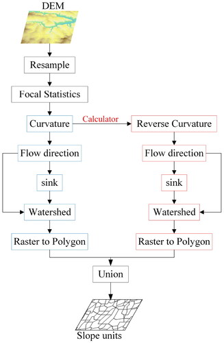
Grid units and slope units are currently two commonly used mapping units. When facing topographically diverse mountainous terrain, slope units can accurately represent the terrain characteristics of different slope segments, better characterizing the disasters influencing factors (Zhang et al. 2021; Sun et al. 2023). The curvature watershed method is currently the most adopted slope unit division method in most studies (Sun et al. 2020; Lin et al. 2024). Its principle involves calculating the average surface curvature to identify points of abrupt changes in the terrain, which enables the segmentation of watersheds (Yan et al. 2017). In this method, points with extremely high curvature are considered protrusions in the terrain, and the boundaries of concave landform elements are determined by connecting all points of maximum curvature. By identifying terrain transition points using the reversed average curvature and segmenting the watershed, it is possible to obtain the boundaries of convex landform elements. The graphic unit formed by superimposing the boundary of the convex geomorphic element and the boundary of the concave geomorphic element is considered a slope unit. The specific process is illustrated in Figure 4. All steps are implemented by tools in Arcgis software. This method needs to set few parameters, which reduces the influence of human subjectivity. The raster size in the resample step controls the size of slope units, which is set to 200 by experiment. When overlaying positive and negative terrain vectors to form slope units, certain surfaces are generated that do not conform to the terrain, such as fragmented surfaces. We eliminate these surfaces by merging slope units with an area less than 900 m² with neighboring slope cells that have the largest area or the longest common boundary. Finally, the study area was broken up into 222,916 slope units.

Figure 4. Flowcharts of slope unit generation.

Flowchart of slope unit generation.

The zonal statistical tool of Arcgis was used to extract features of factors based on slope units. For continuous factors, the attribute value is calculated as the average of all grids corresponding to the slope unit. As for discrete factors, the attribute value is determined by the most frequently occurring value among all grids matching to the slope unit. Moreover, 638 historical landslide surfaces were processed to obtain 864 landslide slope units.

3.2.2. Classifying similar environments

In complex environments, traditional sampling methods for selecting non-landslide samples may not ensure environmental balance with landslide samples. It is necessary to determine different environmental types using geo-environmental consistency constraints and then select the samples. Additionally, the division of slope units can only represent the regional topographical characteristics, without reflecting the geological environmental features at the slope scale. Therefore, using disaster-pregnant environment factors to construct similar environments enables the incorporation of prior knowledge in selecting non-landslide samples. To equally assess the impact of different factor categories on landslides, weights for different categories of disaster-pregnant environment factors were determined based on the results of normalized FRs. The normalization expression is shown in Equation (3). (3) $$\begin{array}{c}{{\mathrm{\text{FR}}}_{\mathit{\text{ij}}}}^{\prime }=\frac{{\mathrm{\text{FR}}}_{\mathit{\text{ij}}}}{\mathrm{\text{max}}\hspace{0.17em}\left({\mathrm{\text{FR}}}_{\mathit{\text{ij}}}\right)-\mathrm{\text{min}}\hspace{0.17em}\left({\mathrm{\text{FR}}}_{\mathit{\text{ij}}}\right)} \end{array}$$(3)

where ${{\mathit{\text{FR}}}_{\mathit{\text{ij}}}}^{\prime }$ denotes the weight between category $j$ of factor $i$ and the typical category of landslides under factor.

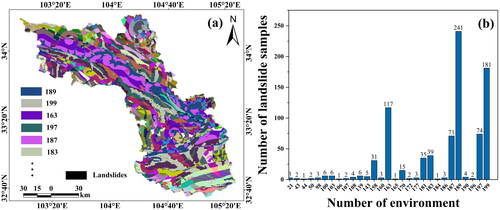
The weight results of disaster-prone environmental factors are shown in Figure 5. According to the four disaster-pregnant environment factor attribute values of slope unit, the class and weight of these values can be determined. Then, a weighted one-hot encoding array of the slope unit is generated to represent the geological environment of the slope unit. Finally, all slope units have been classified into 205 similar environments based on similarity, and the spatial distribution of these similar environments is depicted in Figure 6(a). This can provide prior knowledge for the next step of dataset construction. The distribution of landslide samples in different similar environments is shown in Figure 6(b).

Figure 5. Classes and weights of disaster-pregnant environment factors.

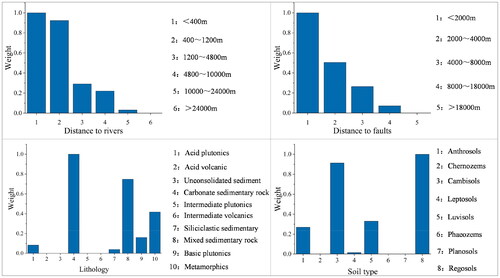
Figure 6. (a) The spatial distribution of similar environments. (b) The number of landslide samples distributed in each environment.

3.2.3. Sample-optimized dataset

We constructed the dataset using a balanced sampling strategy that considers the disaster-pregnant environments similarity, incorporating both landslide and non-landslide samples. Similar environment method (SEM) aims to balance between landslide and non-landslide samples and incorporate prior knowledge to ensure the reliability of the learning process. When assigning labels to samples, the label value for slope units experiencing landslides was set to 1, while the remaining slope units were considered as unlabelled samples. During the process of traversing environments to create the dataset, if there were no landslide samples in a particular environment, that environment was skipped, and the traversal continued. If there was only 1 landslide sample, it was directly placed into the training set. If there were more than 1 landslide samples, they were divided into training and testing sets in a 7:3 ratio. When the number of unlabelled samples in an environment exceeded the number of landslide samples, an equal number of unlabelled samples were randomly selected to serve as non-landslide samples, and their labels were set to 0. If the number of non-landslide samples selected was less than 2, they were directly placed into the training set. If the number of selected non-landslide samples was greater than or equal to 2, they were divided into training and testing sets in a 7:3 ratio. At this point, the training and testing sets covered all environments with existing landslide samples.

Additionally, we compared datasets constructed through random method (RM) with datasets constructed based on the similarity of disaster-pregnant environments. In random sampling, landslide samples were obtained from landslide inventory data, and an equal number of non-landslide samples randomly selected from outside the known landslide samples. Subsequently, the known samples were randomly divided into 70% for training and 30% for testing.

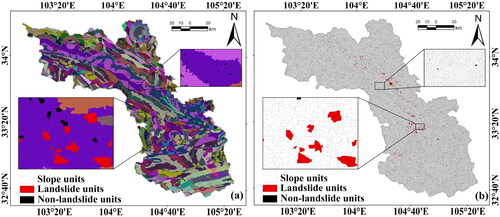
Figure 7(a) shows the spatial distribution of non-landslide samples that were selected using the balanced sampling strategy and environmental constraints, while Figure 7(b) shows the spatial distribution of randomly selected non-landslide samples. The spatial distribution maps indicate that sampling within similar environments enables the selection of non-landslide samples from nearby and distant similar environments. This enables the deep learning models to more effectively learn landslide features.

Figure 7. Distribution of sample sites: (a) non-landslide samples based on SEM, (b) non-landslide samples based on RM.

3.3. Landslide susceptibility assessment based on ensemble learning

3.3.1. Base model

3.3.1.1. MLP

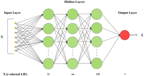
MLP is a commonly used feedforward neural network employed for solving classification and regression problems (Buscema 2002). MLP is composed of multiple neural network layers, with every layer containing neurons (Figure 8). Every neuron is connected to all the neurons in the adjacent layers, forming a fully connected structure. Each connection has a weight that can be adjusted to regulate the strength of signal transmission. The fundamental principle behind MLP is to progressively learn the complicated correlations between input and output through iterative training (He et al. 2023). Every neuron has an activation function to calculate the output value. During the training process, the network adjusts its parameters using the backpropagation algorithm to make accurate predictions for new input data.

Figure 8. The structure of MLP model.

The formula for the input layer to the hidden layer is provided by Equation (4)(4) $$\begin{array}{c}H=f\left(W_h\bullet X+b_h\right)\end{array}$$(4) . (4) $$\begin{array}{c}H=f\left(W_h\bullet X+b_h\right)\end{array}$$(4)

where $H$ denotes the output value for hidden layer; $W_h$ and $b_h$ denote the matching weights and biases, respectively; $h$ denotes the number of neurons for hidden layer.

The process from the hidden layer to the output layer is provided by Equation (5)(5) $$\begin{array}{c}O=F\left(W_o\bullet H+b_o\right)\end{array}$$(5) . (5) $$\begin{array}{c}O=F\left(W_o\bullet H+b_o\right)\end{array}$$(5)

where $O$ denotes the predicted value; $W_o$ and $b_o$ denote the matching weights and biases, respectively.

3.3.1.2. CNN

CNN is a deep learning model specialized to deal with data with a grid structure (LeCun et al. 2015). It has achieved tremendous success in computer vision, image processing, and other applications. In addition to the common input and output layers shared with ordinary neural networks, it also contains convolutional layers, pooling layers, and fully connected layers. The sliding convolutional kernels in the convolutional layers are used to capture primary features from the data. The specific calculation formula is given by Equation (6)(6) $$\begin{array}{c}{C}_j=\sum _i^{N}f\left(w_j\times x_i+b_j\right),j=1,2,\dots ,k\end{array}$$(6) : (6) $$\begin{array}{c}{C}_j=\sum _i^{N}f\left(w_j\times x_i+b_j\right),j=1,2,\dots ,k\end{array}$$(6)

where $k$ denotes the number of convolutional kernels; $C_j$ denotes the output of the $j$-th convolutional kernel; $f$ is the nonlinear activation function; $i$ denotes the spatial position of the convolution operation; $x_i$ denotes the input features to the convolution window; $w_j$ and $b_j$ denote the weight and bias, respectively.

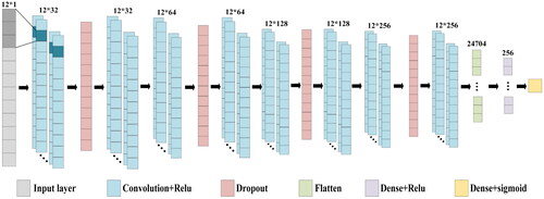
We constructed a CNN model consisting of one-dimensional (1D) convolutional layers, dropout layers, and fully connected layers to predict landslide susceptibility (Figure 9). In the convolutional layers, the input LIFs undergo convolution operations with convolutional kernels to extract low-level features, and then high-level features are obtained by combining of numerous convolutional kernels. The Dropout layer is primarily used to suppress overfitting. For the fully connected layer, the feature maps of the landslide are flattened into a 1D vector. Finally, the sigmoid function outputs the predicted landslide probability.

Figure 9. The structure of CNN model.

3.3.1.3. GRU

GRU is an improvement over the ordinary recurrent neural network model, designed to more effectively capture and leverage long-term dependencies in time series data (Dey and Salem 2017). This improvement enhances the predictive performance. In the structure of the GRU (Figure 10), a gating mechanism has been added, where the update gate $z_t$ determines whether old information is retained and new information is added, and the reset gate $r_t$ determines whether previous information is ignored. Their formula descriptions are shown in Equations (7)(7) $$\begin{array}{c}{z}_t=\sigma \left(U_z{h}_{t-1}+W_z{x}_t+b_z\right)\end{array}$$(7) and (8)(8) $$\begin{array}{c}{r}_t=\sigma \left(U_r{h}_{t-1}+W_r{x}_t+b_r\right)\end{array}$$(8) . ${\tilde{h}}_t$ denotes the status information of the new memory unit at the current time. $h_t$ denotes the updated state information at the current time step; ⊗ denotes element-wise matrix multiplication, then the status update calculation formula is shown in Equations (9)(9) $$\begin{array}{c}{\tilde{h}}_t=\mathrm{\text{tan}}\hspace{0.17em}h\left(U_h\left(r_t\text{⊗}{h}_{t-1}\right)+W_h{x}_t+b_h\right)\end{array}$$(9) and (10)(10) $$\begin{array}{c}{h}_t=z_t{\tilde{h}}_t+\left(1-z_t\right)h_{t-1}\end{array}$$(10) . (7) $$\begin{array}{c}{z}_t=\sigma \left(U_z{h}_{t-1}+W_z{x}_t+b_z\right)\end{array}$$(7) (8) $$\begin{array}{c}{r}_t=\sigma \left(U_r{h}_{t-1}+W_r{x}_t+b_r\right)\end{array}$$(8) where $x_t$ is the current input; $U$ and $W$ are parameter matrices; $b$ is the bias term matrix; $\sigma$ is the sigmoid activation function; $h_{t-1}$ is the status information of the previous moment. (9) $$\begin{array}{c}{\tilde{h}}_t=\mathrm{\text{tan}}\hspace{0.17em}h\left(U_h\left(r_t\text{⊗}{h}_{t-1}\right)+W_h{x}_t+b_h\right)\end{array}$$(9) (10) $$\begin{array}{c}{h}_t=z_t{\tilde{h}}_t+\left(1-z_t\right)h_{t-1}\end{array}$$(10)

Figure 10. The structure of GRU model.

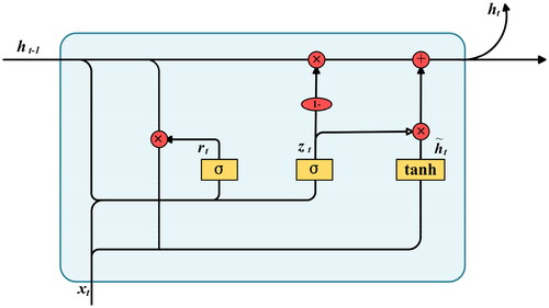
We implemented a three-layer GRU network for taking more stable landslide features. After sorting the LIFs based on their importance, a feature data sequence is formed with a size of (12, 1), where 1 indicates the number of channels.

3.3.2. Ensemble learning methods

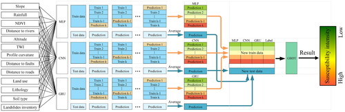
3.3.2.1. Stacking

Stacking ensemble is a type of heterogeneous ensemble model that leverages a meta-learner to fuse different base models together, forming a new model to generate more accurate predictive outcomes (Wolpert 1992). As shown in Figure 11, through cross-validation, this ensemble algorithm predicts the unused samples of the base model to generate the training sample for the meta-learner. Taking k-fold cross-validation as an example, the initial training dataset is divided into k equally sized datasets, $D_1,$ $D_2,$ …, $D_k.$ One of these datasets serves as the primary testing dataset, while the remaining k − 1 datasets serve as the primary training dataset to train the base models. The base models are then used to make predictions on the primary testing dataset, and the predicted values are incorporated into the training dataset for the meta-learner. This process is repeated k times, concatenating to form the training dataset for the meta-learner. Finally, the meta-learner is trained and used for making predictions.

Figure 11. The structure of stacking ensemble learning model.

3.3.2.2. Blending

The blending ensemble is similar to stacking ensemble, as illustrated in Figure 12. It also utilizes a meta-learner to fuse different base models together. The difference lies in the fact that blending does not use cross-validation to create training samples for the meta-learner; instead, it creates a new training dataset using the leave-one-out method on the initial training dataset. In comparison to the stacking ensemble, the blending ensemble is simpler and avoids issues related to information leakage. However, because it does not use the entire training dataset to input the base models, it may encounter overfitting issues.

Figure 12. The structure of blending ensemble learning model.

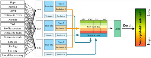
The ensemble learning models and deep learning models in this study were implemented using Python 3.9 and developed using the open frameworks TensorFlow 2.9.1 and Scikit-Learn. An iterative process was used to train and optimize the parameters. The number of folds for cross-validation in stacking ensemble was determined to be 5 through experimentation. The available samples were classified into training and testing datasets and then fed into the MLP, CNN, and GRU models. In both stacking and blending ensemble models, training was conducted using the training dataset, ultimately generating a secondary training dataset. These ensemble methods avoided using the training dataset of the base models directly to create the secondary training dataset, which reduced the overfitting. The predicted results from the base models were aggregated into new features, and the gradient boosting decision trees (GBDT) model was employed as the meta-learner to predict the final result. GBDT belongs to the boosting algorithm family and was introduced by Jerome Friedman in 1999 (Friedman 2001). GDBT iterates through multiple regression trees to fit residuals and continuously reduces residuals to achieve the purpose of joint decision-making. This approach offers good interpretability and robustness. However, this model is rarely applied in LSM (Pham et al. 2021).

3.4. Model evaluation

As the model outputs probability in a range from 0 to 1, the predicted results are classified as landslide or non-landslide using a threshold of 0.5 (Zhao et al., 2022). The landslide susceptibility prediction results for the testing set can be categorized into four groups: true positive (TP)-the actual landslide samples predicted as landslide; true negative (TN)-the actual non-landslide samples predicted as non-landslide; false positive (FP)-the actual non-landslide samples predicted as landslide; false negative (FN)-the actual landslide samples predicted as non-landslide.

Based on the types of susceptibility prediction results, the following metrics are calculated to evaluate the model: accuracy (ACC), which measures the ratio of correctly predicted samples among all samples; precision, which represents the ratio of TP predictions to the total positive predictions in the testing set; recall, which measures the proportion of actual landslide samples that are correctly predicted as landslide points; and F1-score, which is the harmonic mean of precision and recall. The calculation formulas are shown in Equations (11)(11) $$\begin{array}{c}\mathit{\text{ACC}}=\frac{\mathrm{\text{TP}}+\mathrm{\text{TN}}}{\mathrm{\text{TP}}+\mathrm{\text{FP}}+\mathrm{\text{FN}}+\mathrm{\text{TN}}}\end{array}$$(11) –(14)(14) $$\begin{array}{c}F1-\mathit{\text{score}}=2\times \frac{\mathrm{\text{Precision}}\times \mathrm{\text{Recall}}}{\mathrm{\text{Precision}}+\mathrm{\text{Recall}}}\end{array}$$(14) , respectively. (11) $$\begin{array}{c}\mathit{\text{ACC}}=\frac{\mathrm{\text{TP}}+\mathrm{\text{TN}}}{\mathrm{\text{TP}}+\mathrm{\text{FP}}+\mathrm{\text{FN}}+\mathrm{\text{TN}}}\end{array}$$(11) (12) $$\begin{array}{c}\mathit{\text{Precision}}=\frac{\mathrm{\text{TP}}}{\mathrm{\text{TP}}+\mathrm{\text{FP}}}\end{array}$$(12) (13) $$\begin{array}{c}\mathit{\text{Recall}}=\frac{\mathrm{\text{TP}}}{\mathrm{\text{TP}}+\mathrm{\text{FN}}}\end{array}$$(13) (14) $$\begin{array}{c}F1-\mathit{\text{score}}=2\times \frac{\mathrm{\text{Precision}}\times \mathrm{\text{Recall}}}{\mathrm{\text{Precision}}+\mathrm{\text{Recall}}}\end{array}$$(14)

The Receiver Operating Characteristic (ROC) curve is a comprehensive metric that measures the sensitivity and specificity for classification model (He, Yao, et al. 2021). For the ROC curve, the x-axis is the false positive rate (FPR) and the y-axis is the true positive rate (TPR), as defined in Equations (15)(15) $$\begin{array}{c}\mathit{\text{FPR}}=\frac{\mathrm{\text{FP}}}{\mathrm{\text{FP}}+\mathrm{\text{TN}}}\end{array}$$(15) and (16)(16) $$\begin{array}{c}\mathit{\text{TPR}}=\frac{\mathrm{\text{TP}}}{\mathrm{\text{TP}}+\mathrm{\text{FN}}}\end{array}$$(16) . The area under the curve (AUC) of the ROC is employed to measure the model’s ability to generalize, offering an evaluation metric for landslide susceptibility zoning results. (15) $$\begin{array}{c}\mathit{\text{FPR}}=\frac{\mathrm{\text{FP}}}{\mathrm{\text{FP}}+\mathrm{\text{TN}}}\end{array}$$(15) (16) $$\begin{array}{c}\mathit{\text{TPR}}=\frac{\mathrm{\text{TP}}}{\mathrm{\text{TP}}+\mathrm{\text{FN}}}\end{array}$$(16)

4. Results and analysis

4.1. Analysis of landslide influence factors

We calculated the multicollinearity results for LIFs using the Python programming language. As shown in Figure 13(a), rainfall has the highest VIF value (3.004) and the lowest tolerance value (0.333), indicating that all factors fall within an acceptable threshold range. They have good independence and there is no collinearity problem. All factors can be used to train deep learning models.

Figure 13. (a) Multicollinearity evaluation of LIFs. (b) Variable importance of each LIF using random Forest.

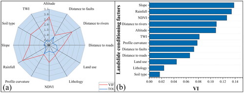
To obtain a more stable and reasonable input features sequence, RF model was employed to calculate the VI of LIFs. Importance ranking results are shown in Figure 13(b), where slope has the highest value (0.1381), and soil type has the lowest value (0.0168). Higher values indicate a stronger correlation with landslides in the region. The ranking factors are passed to the model for subsequent data processing.

To further reveal the relationship between landslides and LIFs, we classified each factor and calculated the FR values for each category. Table 2 shows the FR values for landslide in each category, revealing differences among various categories for each factor. When FR value is higher, which indicates that the area is more prone to landslides. In Bailong River Basin, most landslides occurred in areas with altitudes under 3000 m, possibly due to the prevalence of landslides near riverbanks and these riverbanks are all at lower altitudes. The likelihood of landslides is significant on slopes with a gradient of 30° to 45°. For profile curvature, Bailong River Basin has higher FR values in (−20, 0) and (0, 20). TWI can quantitatively simulate topography and soil moisture within the basin. As the FR value of TWI increases, the landslide area decreases. The rainfall results show that there is an obvious relationship between landslide and rainfall. The highest FR is category of 600–700 mm/year, and more than half of historical landslides are in the category of 700–800 mm/year. The highest FR value in land use is forest land, which accounts for 77% of the study area. Due to the increased air humidity from the strong transpiration in forests, forest areas often experience higher rainfall. Concentrated heavy rainfall is highly likely to trigger landslides. The FR values of NDVI indicate landslides mainly in areas with higher NDVI, reflecting the indirect impact of vegetation growth and coverage on slope stability. For FR values related to lithology, landslides more developed in mixed sedimentary rocks and carbonate sedimentary rocks, which are predominantly distributed near riverbanks. FR values for soil type indicate that landslides tend to occur in conical soil and highly active leached soil, which are also distributed near riverbanks and consist of finer-textured soils. Finer-textured soils have stronger water retention capacity than coarser soils under unsaturated conditions. During heavy rainfall, soils with high water retention capabilities can increase the slope weight and lead to slope movement. FR values related to the distance to faults, rivers, and roads indicate that the landslide decreases with increasing distance. Most landslides occur within 2000 m of rivers and roads, indicating a strong spatial distribution relationship. Roads are typically close to human settlements, highlighting the landslides as a threat to human life and property.

Table 2. Relationship between the historical landslides and LIFs.

Factors	Class	No. of pixels in class	Class (%)	No. of historical landslide pixels in the class	Landslide incidences (%)	FR
Altitude	<1500	2,526,579	12.28%	22,461	23.51%	1.91
	1500–2000	4,120,088	20.03%	31,891	33.37%	1.67
	2000–2500	4,816,270	23.41%	20,928	21.90%	0.94
	2500–3000	4,438,185	21.57%	14,831	15.52%	0.72
	3000–3500	3,098,194	15.06%	4644	4.86%	0.32
	3500–4000	1,344,675	6.54%	787	0.82%	0.13
	4000–4500	225,135	1.09%	13	0.01%	0.01
	>4500	4937	0.02%	0	0.00%	0.00
Slope	<15	2,061,180	10.02%	3990	4.18%	0.42
	15–30	7,692,252	37.39%	23,195	24.27%	0.65
	30–45	9,123,085	44.34%	50272	52.61%	1.19
	45–60	1,611,876	7.83%	16,931	17.72%	2.26
	60–75	84,908	0.41%	1157	1.21%	2.93
	>75	762	0.00%	10	0.01%	2.82
Profile curvature	< −40	6	0.00%	0	0.00%	0.00
	(−40, −20)	142	0.00%	0	0.00%	0.00
	(−20,0)	10,111,163	49.15%	45,233	47.33%	0.96
	(0,20)	10,462,576	50.85%	50,322	52.66%	1.04
	(20,40)	170	0.00%	0	0.00%	0.00
	>40	6	0.00%	0	0.00%	0.00
TWI	<4	10,839,476	52.69%	60,057	62.85%	1.19
	4–8	9,183,810	44.64%	34,562	36.17%	0.81
	8–12	446,010	2.17%	868	0.91%	0.42
	12–16	1641	0.01%	0	0.00%	0.00
	16–20	76,381	0.37%	48	0.05%	0.14
	>20	26,744	0.13%	20	0.02%	0.16
Rainfall	<600	12,203	0.06%	0	0.00%	0.00
	600 − 700	917,275	4.46%	28,741	30.08%	6.75
	700 − 800	10,949,641	53.22%	45,940	48.08%	0.90
	800 − 900	8,382,998	40.75%	20,631	21.59%	0.53
	>900	311,946	1.52%	244	0.25%	0.17
Land use	Cultivated land	3,620,866	17.60%	7304	7.64%	0.43
	Forest	15,927,658	77.42%	86,255	90.27%	1.17
	Grass land	814,889	3.96%	1335	1.40%	0.35
	Shrubland	12,462	0.06%	100	0.10%	1.73
	Wetland	123	0.00%	0	0.00%	0.00
	Water body	68,117	0.33%	110	0.12%	0.35
	Artificial surfaces	129,949	0.63%	451	0.47%	0.75
NDVI	0–0.1	1336	0.01%	0	0.00%	0.00
	01–0.2	72,918	0.35%	11	0.01%	0.03
	0.2–0.3	166,672	0.81%	157	0.16%	0.20
	0.3–0.4	647,169	3.15%	6357	6.65%	2.11
	0.4–0.5	3,258,216	15.84%	33,058	34.60%	2.18
	0.5–0.6	6,568,837	31.93%	32,501	34.01%	1.07
	0.6–0.7	7,316,562	35.56%	20,532	21.49%	0.60
	0.7–0.8	2,535,863	12.33%	2939	3.08%	0.25
	>0.8	6491	0.03%	0	0.00%	0.00
Lithology	Acid plutonics	198,331	0.96%	170	0.18%	0.18
	Acid volcanics	21,699	0.11%	0	0.00%	0.00
	Unconsolidated sediment	45,749	0.22%	0	0.00%	0.00
	Carbonate sedimentary rock	2,831,949	13.76%	28,972	30.32%	2.20
	Intermediate plutonics	52,083	0.25%	0	0.00%	0.00
	Intermediate volcanics	3526	0.02%	0	0.00%	0.00
	Siliciclastic sedimentary	1,366,616	6.64%	553	0.58%	0.09
	Mixed sedimentary rock	6,527,761	31.73%	49,917	52.24%	1.65
	Basic plutonics	9,419,241	45.78%	15,485	16.21%	0.35
	Metamorphics	107,108	0.52%	458	0.48%	0.92
Soil type	Anthrosols	114,800	0.56%	317	0.33%	0.59
	Chernozems	157,035	0.76%	0	0.00%	0.00
	Cambisols	5,627,339	27.35%	52,636	55.08%	2.01
	Leptosols	1,785,216	8.68%	262	0.27%	0.03
	Luvisols	12,251,539	59.55%	41,401	43.33%	0.73
	Phaeozems	537,739	2.61%	0	0.00%	0.00
	Planosols	8676	0.04%	0	0.00%	0.00
	Regosols	91,720	0.45%	939	0.98%	2.21
Distance to roads	<1500	12,824,506	62.33%	72,968	76.36%	1.23
	1500–3000	5,412,182	26.31%	18,669	19.54%	0.74
	3000–4500	1,607,589	7.81%	3883	4.06%	0.52
	4500–6000	545,821	2.65%	35	0.04%	0.01
	6000–7500	161,206	0.78%	0	0.00%	0.00
	>7500	22,760	0.11%	0	0.00%	0.00
Distance to rivers	<400	1,099,650	5.34%	16,363	17.14%	3.21
	400–1200	2,060,191	10.01%	28,284	29.62%	2.96
	1200–4800	6,719,409	32.66%	29,161	30.54%	0.94
	4800–10,000	5,963,859	28.99%	19,605	20.53%	0.71
	10000–24,000	4,602,919	22.37%	2142	2.24%	0.10
	>24,000	128,034	0.62%	0	0.00%	0.00
Distance to faults	<2000	10,353,749	50.32%	73,395	76.81%	1.53
	2000–4000	3,630,365	17.65%	13,003	13.61%	0.77
	4000–8000	4,270,319	20.76%	8018	8.39%	0.40
	8000–18,000	2,247,467	10.92%	1139	1.19%	0.11
	>18000	72,163	0.35%	0	0.00%	0.00

4.2. LSM

Results from the ensemble learning models were visually processed to generate LSMs. Landslide probability was classified into five susceptibility levels using the natural breaks method with ArcGIS software: very low, low, moderate, high, and very high (Wang et al. 2019). Figure 14 illustrates LSMs obtained using different methods for Bailong River Basin. To demonstrate the advantages of similar environmental sampling, ensemble learning models were also trained using the dataset with non-landslide samples randomly sampled.

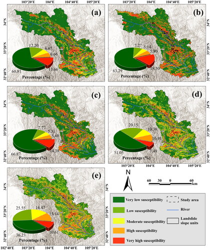
Figure 14. LSMs Generated using (a) stacking based on the RM, (b) blending based on the RM, (c) stacking based on the SEM, and (d) blending based on the SEM. Regions A and B are zoomed in to provide an intuitive visualization of LSM using different non-landslide sampling methods. The lowest subfigure shows the proportion of area at each landslide susceptibility level.

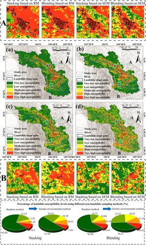
LSMs based on stacking and blending ensemble models with similar environment sampling (Figure 14c,d) show spatial similarities. When similar environments are considered in distant areas, the distribution of very high susceptibility is more reasonable. Apart from the historical landslides surroundings and the banks of central rivers, very high susceptibility is also observed in the southeast coastal and some mountainous areas, and the northwest mountainous regions. LSMs generated using stacking and blending ensembles with random sampling (Figure 14a,b) show a high concentration of very high susceptibility around historical landslides and along central riverbanks. These maps show underfitting in areas lacking landslide samples. In contrast, proposed non-landslide sample selection method based on similar environments perfectly overcomes this drawback. Additionally, the stacking ensemble model with random sampling generates many false positives globally, where very high susceptibility is generated in very small regions, while the blending ensemble model does not exhibit such occurrences. In the subgraph for region A, non-landslide samples distribution based on random sampling appears to be random and less numerous, resulting in a larger very high susceptibility area around landslide samples. However, non-landslide samples distribution based on similar environmental sampling shows some correlation with landslide. Compared to random sampling, very high susceptibility area around landslide samples significantly decreases, yielding more accurate results. Similar findings are shown in region B, indicating that the optimized dataset enables the models to more thoroughly learn landslide features, leading to better landslide predictions. Through sample optimization, the proportions of very low susceptibility in both ensemble models decreased by 14.8 and 24.43, while the proportions of low, moderate, and high susceptibility increased. For stacking ensemble model, the proportion of individuals with very high susceptibility decreased by 2.81, consistent with region A and B. For blending ensemble model, the proportion of very high susceptibility decreased by 0.96, indicating differences in the ability to identify very high susceptibility between the two models.

4.3. Model evaluation and precision analysis

Predictive results were evaluated for accuracy to quantify the predictive ability of the models. We compared ensemble models based on different non-landslide sample sampling methods using the accuracy metrics shown in Table 3. In the case of similar environment sampling of non-landslide samples, stacking ensemble demonstrates higher values for ACC, F1-score, and AUC compared to the blending ensemble. Similar results are observed when using random sampling. The stacking ensemble demonstrates superior predictive capability compared to the blending ensemble, resulting in better performance in landslide susceptibility assessment. For both stacking and blending ensemble models, ACC, F1-score, and AUC are slightly higher with random sampling than with similar environmental sampling. However, the spatial performance of LSM is poorer in random sampling, and they do not enhance predictions in regions with scarce landslide samples. Since machine learning models are data-driven and feature acquisition depends on training dataset. When the parameters and structure of a model are the same but trained on different datasets, models may demonstrate varying degrees of learning. Therefore, relying solely on the evaluation metrics may not be sufficient to determine the superiority or inferiority of a dataset construction method.

Table 3. Accurate metrics for ensemble models using different testing dataset.

		ACC	Precision	Recall	F1-score	AUC
SEM	Stacking	80.11%	0.7630	0.8736	0.8146	0.88
	Blending	79.37%	0.7883	0.8030	0.7956	0.85
RM	Stacking	81.16%	0.8031	0.8485	0.8252	0.89
	Blending	80.85%	0.7656	0.8523	0.8066	0.87

5. Discussion

5.1. Random sampling and similar environment sampling

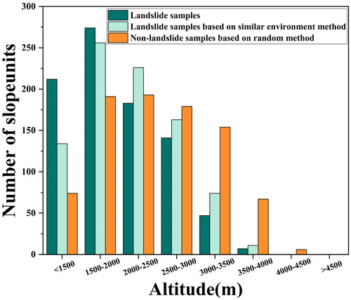
Non-landslide samples selection introduces significant uncertainty, and different non-landslide sample selection methods have a noticeable impact on LSM (Dou et al. 2023). RM is the most common method for selecting non-landslide samples (Yu et al. 2024; Xiao et al. 2024). Landslide samples are not uniformly distributed globally, non-landslide samples are uniformly distributed globally. Their only association with the landslide samples is the equal number. When the study area is larger and the environment is more complex, the RM will have a large randomness and increase the uncertainty (Chang et al. 2023). In Figure 15, non-landslide samples selection based on RM is not influenced by altitude and does not show similarity to landslide samples distribution. This inevitably leads to underfitting in areas with a shortage of samples. However, non-landslide samples selection constrained by disaster-pregnant environment factors can better choose a reasonable number of non-landslide samples within each altitude range. This results in samples with strong robustness (Liu et al. 2022). In LSMs, ensemble models trained using RM show a very high susceptibility distribution mainly around historical landslides and along the central rivers. Underfitting also occurs in areas where landslide samples are scarce. In contrast, the proposed non-landslide sample selection based on similar environments perfectly overcomes this drawback. When comparing the spatial distribution and proportion of susceptibility levels trained using two different sampling methods for stacking and blending ensemble models, it is evident that similar environmental sampling can provide rich information, enabling the model to better discriminate samples and make accurate predictions. It identified very high susceptibility areas far from the landslide samples across different spatial regions.

Figure 15. The distribution of samples in each class of altitude.

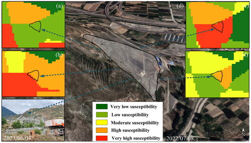
Furthermore, LSM was validated by Google Earth images and field verifications. Figures 16 and 17 depict landslides at two different locations in the same environment (ID 189), each situated in different counties, with no landslide and non-landslide samples used in training models around them. In Figure 16, both ensemble models based on RM predicted very low susceptibility, while the stacking ensemble model based on SEM predicted very high susceptibility, and the blending ensemble model predicted high susceptibility. In Figure 17, the stacking ensemble model based on RM predicted low susceptibility, the blending ensemble model predicted high susceptibility, and the stacking ensemble model based on SEM predicted very high susceptibility, while the blending ensemble model predicted high susceptibility. This demonstrates that models trained by similar environmental sampling dataset can identify distant landslides whose environment is similar to existing landslide samples. It is more comprehensive to learn the features from both landslide and non-landslide samples.

Figure 16. (a) LSM generated using stacking based on RM, (b) LSM generated using blending based on RM, (c) field verification photograph, (d) Google earth image, (e) LSM generated using stacking based on SEM, (f) LSM generated using blending based on SEM.

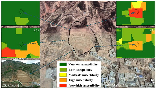
Figure 17. (a) LSM generated using stacking based on RM, (b) LSM generated using blending based on RM, (c) field verification photograph, (d) Google Earth image, (e) LSM generated using stacking based on SEM, (f) LSM generated using blending based on SEM.

5.2. Base models and ensemble models

Deep learning is widely used in landslide susceptibility assessment, different types of deep learning pay different attention to features (He, Zhao, et al. 2021; Zhao et al. 2024; Achu et al. 2024). When the study area is larger and its environment is more complex, the prediction results of a single model are weakly supported for landslide prevention and control. In contrast, stacking and blending ensemble learning utilize meta-learners to correct deficiencies in the base model learning process, resulting in higher predictive capabilities (Fang et al. 2021). In Figure 18, the LSM of MLP shows very high susceptibility near the bottom of the river, while CNN and GRU have fewer very high susceptibility areas in the same region. Additionally, MLP has fewer areas of very high susceptibility near the southwest edge, while CNN and GRU have more in the same region, indicating a bias in the attention of different models towards to landslide-prone areas. Stacking and blending ensemble collectively address this situation by reducing the range of very high susceptibility in the same locations. This suggests that ensemble learning model can prioritize to detect areas with the highest probability of landslide (Zeng, Wu, et al. 2023). In addition, the proportion of very high susceptibility in the ensemble model decreased compared to the base model. Ensemble models show a significantly reduced area of very high susceptibility around historical landslides compared to base models. This further emphasizes the higher accuracy of stacking ensemble, which can facilitate landslide prevention efforts by relevant authorities.

Figure 18. LSM generated using (a) MLP, (b) CNN, (c) GRU, (d) stacking and (e) blending.

In Table 4 and Figure 19, the evaluation metrics for base models and ensemble models are summarized. Stacking outperforms blending and base models in terms of ACC, F1-score, and AUC. We calculated the FR of historical landslides in the LSM levels for each model using ArcGIS software (Figure 20). For very high susceptibility, FR values for MLP, CNN, GRU, stacking ensemble, and blending ensemble are 5.76, 4.81, 5.73, 10.49, and 7.36, respectively. Stacking ensemble is 3.13 higher than blending ensemble. Both the metrics and FR results indicate that stacking exhibits higher accuracy. This is attributed to the use of cross-validation to generate training data for the meta-learner in stacking ensemble model. Cross-validation enables the base models to thoroughly learn the environmental features of the samples, resulting in more accurate predictions. Stacking ensemble models have great potential for application in predicting complex areas or new scenarios.

Figure 19. ROC curves of different models using testing dataset.

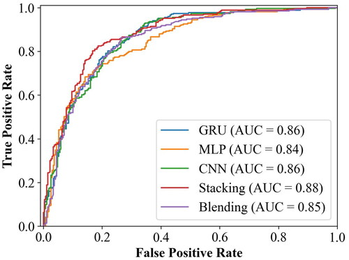
Figure 20. FR values for the levels of landslide susceptibility across different models.

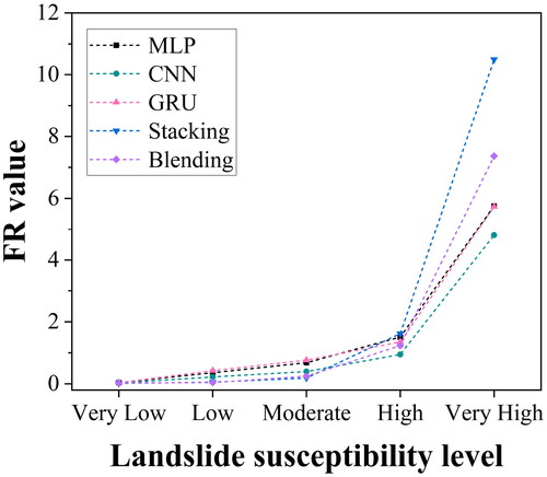
Table 4. Accurate metrics for each model using testing dataset based on SEM.

	Model	ACC	Precision	Recall	F1-score
Base model	MLP	75.28%	0.7313	0.7992	0.7638
	CNN	78.81%	0.7558	0.8513	0.8007
	GRU	78.81%	0.7645	0.8327	0.7971
Ensemble model	Stacking	80.11%	0.7630	0.8736	0.8146
	Blending	79.37%	0.7883	0.8030	0.7956

6. Conclusion

Taking Bailong River Basin with complex environments as an example, this study presents a novel non-landslide sample sampling method and uses ensemble learning methods for landslide susceptibility assessment. Based on slope units, LIFs such as distance to faults, distance to rivers, lithology, and soil type were collected as landslide-pregnant environmental factors. Considering environmental consistency constraints, a dataset was obtained by selecting an equal number of non-landslide samples to match the landslide samples distribution in similar environments. The performance of the proposed SEM in landslide susceptibility assessment was evaluated using the Stacking and Blending ensemble models. The main conclusions are as follows:

1. Comparing the RM and SEM datasets and their corresponding LSM results, the non-landslide samples selected by SEM method exhibit less randomness and uncertainty, and the use of the SEM datasets can improve the prediction results of sample-scarce areas. Considering consistent geographic constraints is an effective method to solve the uncertainty of non-landslide sample selection.

2. Comparing the base models and the ensemble models on SEM, the stacking ensemble demonstrated the highest prediction accuracy, with an ACC of 80.11% and an AUC of 0.88. Heterogeneous ensemble learning models can effectively enhance predictive abilities of base models and more accurately reflect the landslide susceptibility in the study area.

3. In complex environments, sample optimization selection with prior knowledge and heterogeneous ensemble learning model can be adopted to solve the underfitting in sample-scarce areas. The combination of these two methods can obtain more scientific and accurate LSM, which holds significant theoretical and practical value for reducing landslide disaster losses and improving the efficiency of landslide disaster prevention and control.

Disclosure statement

The authors declare that they have no known competing financial interests or personal relationships that have appeared to influence the work reported in this paper.

Data availability statement

The datasets used or analysed during this study are available from the corresponding author on reasonable request.

Additional information

Funding

This work was supported in part by the Gansu Science and Technology Program under Grant 23JRRA881, in part by the National Natural Scientific Foundation of China under Grant 42201459, in part by the Key Research and Development Project of Lanzhou Jiao Tong University under Grant LZJTU-ZDYF2301, and in part by the Key Science and Technology Project of Jiangxi Provincial Department of Natural Resources, Research on Key Technologies of Ground Settlement Monitoring and Landslide Monitoring and Early Warning Model in Nanchang City Based on InSAR under Grant ZRKJ20232424.

References

- Achu AL, Aju CD, Di Napoli M, Prakash P, Gopinath G, Shaji E, Chandra V. 2023. Machine-learning based landslide susceptibility modelling with emphasis on uncertainty analysis. Geosci Front. 14(6):101657. doi: 10.1016/j.gsf.2023.101657.
- Achu AL, Thomas J, Aju CD, Remani PK, Gopinath G. 2023. Performance evaluation of machine learning and statistical techniques for modelling landslide susceptibility with limited field data. Earth Sci Inform. 16(1):1025–1039. doi: 10.1007/s12145-022-00910-8.
- Achu AL, Thomas J, Aju CD, Vijith H, Gopinath G. 2024. Redefining landslide susceptibility under extreme rainfall events using deep learning. Geomorphology. 448:109033. doi: 10.1016/j.geomorph.2023.109033.
- Buscema M. 2002. A brief overview and introduction to artificial neural networks. Subst Use Misuse. 37(8–10):1093–1148. doi: 10.1081/JA-120004171.
- Chang Z, Du Z, Zhang F, Huang F, Chen J, Li W, Guo Z. 2020. Landslide susceptibility prediction based on remote sensing images and GIS: comparisons of supervised and unsupervised machine learning models. Remote Sensing. 12(3):502. doi: 10.3390/rs12030502.
- Chang Z, Huang J, Huang F, Bhuyan K, Meena SR, Catani F. 2023. Uncertainty analysis of non-landslide sample selection in landslide susceptibility prediction using slope unit-based machine learning models. Gondwana Res. 117:307–320. doi: 10.1016/j.gr.2023.02.007.
- Chen T, Gao X, Liu G, Wang C, Zhao Z, Dou J, Niu R, Plaza AJ. 2024. BisDeNet: a new lightweight deep learning-based framework for efficient landslide detection. IEEE J Sel Top Appl Earth Observ Remote Sensing. 17:3648–3663. doi: 10.1109/JSTARS.2024.3351873.
- Chen T, Wang Q, Zhao Z, Liu G, Dou J, Plaza A. 2024. LCFSTE: landslide conditioning factors and swin transformer ensemble for landslide susceptibility assessment. IEEE J Sel Top Appl Earth Observations Remote Sensing. 17:6444–6454. doi: 10.1109/JSTARS.2024.3373029.
- Chen W, Xie X, Wang J, Pradhan B, Hong H, Bui DT, Duan Z, Ma J. 2017. A comparative study of logistic model tree, random forest, and classification and regression tree models for spatial prediction of landslide susceptibility. CATENA. 151:147–160. doi: 10.1016/j.catena.2016.11.032.
- Dai K, Chen C, Shi X, Wu M, Feng W, Xu Q, Liang R, Zhuo G, Li Z. 2023. Dynamic landslides susceptibility evaluation in Baihetan Dam area during extensive impoundment by integrating geological model and InSAR observations. Int J Appl Earth Obs Geoinf. 116:103157. doi: 10.1016/j.jag.2022.103157.
- Dai K, Li Z, Xu Q, Tomas R, Li T, Jiang L, Zhang J, Yin T, Wang H. 2023. Identification and evaluation of the high mountain upper slope potential landslide based on multi-source remote sensing: the Aniangzhai landslide case study. Landslides. 20(7):1405–1417. doi: 10.1007/s10346-023-02044-4.
- Dey R, Salem FM. 2017. Gate-variants of Gated Recurrent Unit (GRU) neural networks. In: 2017 IEEE 60th International Midwest Symposium on Circuits and Systems (MWSCAS). Boston, MA: IEEE. p. 1597–1600. doi: 10.1109/MWSCAS.2017.8053243.
- Dou H, He J, Huang S, Jian W, Guo C. 2023. Influences of non-landslide sample selection strategies on landslide susceptibility mapping by machine learning. Geomatics Nat Hazards Risk. 14(1):2285719. doi: 10.1080/19475705.2023.2285719.
- Dou J, Yunus AP, Bui DT, Merghadi A, Sahana M, Zhu Z, Chen C-W, Han Z, Pham BT. 2020. Improved landslide assessment using support vector machine with bagging, boosting, and stacking ensemble machine learning framework in a mountainous watershed, Japan. Landslides. 17(3):641–658. doi: 10.1007/s10346-019-01286-5.
- Du J, Glade T, Woldai T, Chai B, Zeng B. 2020. Landslide susceptibility assessment based on an incomplete landslide inventory in the Jilong Valley, Tibet, Chinese Himalayas. Eng Geol. 270:105572. doi: 10.1016/j.enggeo.2020.105572.
- Fang Z, Wang Y, Peng L, Hong H. 2021. A comparative study of heterogeneous ensemble-learning techniques for landslide susceptibility mapping. Int J Geogr Inf Sci. 35(2):321–347. doi: 10.1080/13658816.2020.1808897.
- Friedman JH. 2001. Greedy function approximation: a gradient boosting machine. Ann. Statist. 29(5):1189–1232. doi: 10.1214/aos/1013203451.
- Gao B,He Yi,Chen X,Chen H,Yang W,Zhang L. 2024. A Deep Neural Network Framework for Landslide Susceptibility Mapping by Considering Time-Series Rainfall. IEEE J Sel Top Appl Earth Observations Remote Sensing. 17:5946–5969. 10.1109/JSTARS.2024.3370218.
- Gao B, He Y, Chen X, Zheng X, Zhang L, Zhang Q, Lu J. 2023. Landslide risk evaluation in Shenzhen based on stacking ensemble learning and InSAR. IEEE J Sel Top Appl Earth Observ Remote Sensing. 16:1–18. doi: 10.1109/JSTARS.2023.3291490.
- He Y, Wang W, Zhang L, Chen Y, Chen Y, Chen B, He X, Zhao Z. 2023. An identification method of potential landslide zones using InSAR data and landslide susceptibility. Geomatics Nat Hazards Risk. 14(1):2185120. doi: 10.1080/19475705.2023.2185120.
- He Y, Yao S, Yang W, Yan H, Zhang L, Wen Z, Zhang Y, Liu T. 2021. An extraction method for glacial lakes based on Landsat-8 imagery using an improved U-Net network. IEEE J Sel Top Appl Earth Observ Remote Sensing. 14:6544–6558. doi: 10.1109/JSTARS.2021.3085397.
- He Y, Zhao Z, Yang W, Yan H, Wang W, Yao S, Zhang L, Liu T. 2021. A unified network of information considering superimposed landslide factors sequence and pixel spatial neighbourhood for landslide susceptibility mapping. Int J Appl Earth Obs Geoinf. 104:102508. doi: 10.1016/j.jag.2021.102508.
- He Y, Zhao Z, Zhu Q, Liu T, Zhang Q, Yang W, Zhang L, Wang Q. 2024. An integrated neural network method for landslide susceptibility assessment based on time-series InSAR deformation dynamic features. Int J Digital Earth. 17(1):2295408. doi: 10.1080/17538947.2023.2295408.
- Huang F, Cao Z, Guo J, Jiang S-H, Li S, Guo Z. 2020. Comparisons of heuristic, general statistical and machine learning models for landslide susceptibility prediction and mapping. CATENA. 191:104580. doi: 10.1016/j.catena.2020.104580.
- Huang F, Pan L, Yao C, Zhou C, Jiang Q, Chang Z. 2021. Landslide susceptibility prediction modelling based on semi-supervised machine learning. J Zhejiang Univ Eng Sci. 55:1705–1713. doi: 10.3785/j.issn.1008-973X.2021.09.012.
- Huang Y, Zhao L. 2018. Review on landslide susceptibility mapping using support vector machines. CATENA. 165:520–529. doi: 10.1016/j.catena.2018.03.003.
- Karaman MO, Çabuk SN, Pekkan E. 2022. Utilization of frequency ratio method for the production of landslide susceptibility maps: karaburun Peninsula case, Turkey. Environ Sci Pollut Res Int. 29(60):91285–91305. doi: 10.1007/s11356-022-21931-2.
- LeCun Y, Bengio Y, Hinton G. 2015. Deep learning. Nature. 521(7553):436–444. doi: 10.1038/nature14539.
- Li C, Wang M, Liu K. 2018. A decadal evolution of landslides and debris flows after the Wenchuan earthquake. Geomorphology. 323:1–12. doi: 10.1016/j.geomorph.2018.09.010.
- Lin S, Wang X, Nan C. 2024. Slope unit-based genetic landform mapping on Tibetan plateau – a terrain unit-based framework for large spatial scale landform classification. CATENA. 236:107757. doi: 10.1016/j.catena.2023.107757.
- Liu J, Liang E, Xu S, Liu M, Wang Y, Zhang F, Luo A. 2022. Multi-kernel support vector machine considering sample optimization selection for analysis and evaluation of landslide disaster susceptibility. Acta Geod Cartogr Sin. 51(10):2034–2045. doi: 10.11947/1.AGCS,2022.20220326.
- Lv L, Chen T, Dou J, Plaza A. 2022. A hybrid ensemble-based deep-learning framework for landslide susceptibility mapping. Int J Appl Earth Obs Geoinf. 108:102713. doi: 10.1016/j.jag.2022.102713.
- Ma Z, Mei G, Piccialli F. 2021. Machine learning for landslides prevention: a survey. Neural Comput Applic. 33(17):10881–10907. doi: 10.1007/s00521-020-05529-8.
- Merghadi A, Abderrahmane B, Tien Bui D. 2018. Landslide susceptibility assessment at Mila Basin (Algeria): a comparative assessment of prediction capability of advanced machine learning methods. IJGI. 7(7):268. doi: 10.3390/ijgi7070268.
- Pham QB, Achour Y, Ali SA, Parvin F, Vojtek M, Vojteková J, Al-Ansari N, Achu AL, Costache R, Khedher KM, et al. 2021. A comparison among fuzzy multi-criteria decision making, bivariate, multivariate and machine learning models in landslide susceptibility mapping. Geomatics Nat Hazards Risk. 12(1):1741–1777. doi: 10.1080/19475705.2021.1944330.
- Sun D, Gu Q, Wen H, Xu J, Zhang Y, Shi S, Xue M, Zhou X. 2023. Assessment of landslide susceptibility along mountain highways based on different machine learning algorithms and mapping units by hybrid factors screening and sample optimization. Gondwana Res. 123:89–106. doi: 10.1016/j.gr.2022.07.013.
- Sun X, Chen J, Han X, Bao Y, Zhou X, Peng W. 2020. Landslide susceptibility mapping along the upper Jinsha River, south-western China: a comparison of hydrological and curvature watershed methods for slope unit classification. Bull Eng Geol Environ. 79(9):4657–4670. doi: 10.1007/s10064-020-01849-0.
- Trinh T, Luu BT, Nguyen DH, Le THT, Pham SV, VuongThi N. 2023. A study of non-landslide samples and weights for mapping landslide susceptibility using regression and clustering methods. Earth Sci Inform. 16(4):4009–4034. doi: 10.1007/s12145-023-01144-y.
- Wang Y, Fang Z, Hong H. 2019. Comparison of convolutional neural networks for landslide susceptibility mapping in Yanshan County, China. Sci Total Environ. 666:975–993. doi: 10.1016/j.scitotenv.2019.02.263.
- Wang Y, Feng L, Li S, Ren F, Du Q. 2020. A hybrid model considering spatial heterogeneity for landslide susceptibility mapping in Zhejiang Province, China. CATENA. 188:104425. doi: 10.1016/j.catena.2019.104425.
- Wei A, Yu K, Dai F, Gu F, Zhang W, Liu Y. 2022. Application of tree-based ensemble models to landslide susceptibility mapping: a comparative study. Sustainability. 14(10):6330. doi: 10.3390/su14106330.
- Wolpert DH. 1992. Stacked generalization. Neural Netw. 5(2):241–259. doi: 10.1016/S0893-6080(05)80023-1.
- Xiao X, Zou Y, Huang J, Luo X, Yang L, Li M, Yang P, Ji X, Li Y. 2024. An interpretable model for landslide susceptibility assessment based on Optuna hyperparameter optimization and Random Forest. Geomatics Nat Hazards Risk. 15(1):2347421. doi: 10.1080/19475705.2024.2347421.
- Yan G, Liang S, Zhao H. 2017. An approach to improving slope unit division using GIS technique. Sci Geogr Sin. 37:1764–1770. doi: 10.13249/j.cnki.sgs.2017.11.019.
- Yu L, Wang Y, Pradhan B. 2024. Enhancing landslide susceptibility mapping incorporating landslide typology via stacking ensemble machine learning in Three Gorges Reservoir, China. Geosci Front. 15(4):101802. doi: 10.1016/j.gsf.2024.101802.
- Zeng T, Glade T, Xie Y, Yin K, Peduto D. 2023. Deep learning powered long-term warning systems for reservoir landslides. Int J Disaster Risk Reduct. 94:103820. doi: 10.1016/j.ijdrr.2023.103820.
- Zeng T, Guo Z, Wang L, Jin B, Wu F, Guo R. 2023. Tempo-Spatial Landslide Susceptibility Assessment from the Perspective of Human Engineering Activity. Remote Sensing. 15(16):4111. doi: 10.3390/rs15164111.
- Zeng T, Jin B, Glade T, Xie Y, Li Y, Zhu Y, Yin K. 2024. Assessing the imperative of conditioning factor grading in machine learning-based landslide susceptibility modeling: A critical inquiry. CATENA. 236:107732. doi: 10.1016/j.catena.2023.107732.
- Zeng T, Wu L, Hayakawa YS, Yin K, Gui L, Jin B, Guo Z, Peduto D. 2024. Advanced integration of ensemble learning and MT-InSAR for enhanced slow-moving landslide susceptibility zoning. Eng Geol. 331:107436. doi: 10.1016/j.enggeo.2024.107436.
- Zeng T, Wu L, Peduto D, Glade T, Hayakawa YS, Yin K. 2023. Ensemble learning framework for landslide susceptibility mapping: different basic classifier and ensemble strategy. Geosci Front. 14(6):101645. doi: 10.1016/j.gsf.2023.101645.
- Zhang Q, He Y, Zhang L, Lu J, Gao B, Yang W, Chen H, Zhang Y. 2024. A landslide susceptibility assessment method considering the similarity of geographic environments based on graph neural network. Gondwana Res. 132:323–342. doi: 10.1016/j.gr.2024.04.013.
- Zhang S, Ma Z, Li Y, Hu K, Zhang Q, Li L. 2021. A grid-based physical model to analyze the stability of slope unit. Geomorphology. 391:107887. doi: 10.1016/j.geomorph.2021.107887.
- Zhao Z,He Yi,Yao S,Yang W,Wang W,Zhang L,Sun Q. 2022. A comparative study of different neural network models for landslide susceptibility mapping. Adv. Space Res. 70(2):383–401. 10.1016/j.asr.2022.04.055.
- Zhao Z, Chen T, Dou J, Liu G, Plaza A. 2024. Landslide susceptibility mapping considering landslide local-global features based on CNN and transformer. IEEE J Sel Top Appl Earth Observ Remote Sensing. 17:7475–7489. doi: 10.1109/JSTARS.2024.3379350.
- Zhou C, Yin K, Cao Y, Ahmed B, Li Y, Catani F, Pourghasemi HR. 2018. Landslide susceptibility modeling applying machine learning methods: a case study from Longju in the Three Gorges Reservoir area, China. Comput Geosci. 112:23–37. doi: 10.1016/j.cageo.2017.11.019.
- Zhu Q, Chen L, Hu H, Pirasteh S, Li H, Xie X. 2020. Unsupervised feature learning to improve transferability of landslide susceptibility representations. IEEE J Sel Top Appl Earth Observ Remote Sensing. 13:3917–3930. doi: 10.1109/JSTARS.2020.3006192.
- Zhu Q, Zeng H, Ding Y, Xie X, Liu F, Zhang L, Li H, Hu H, Zhang J, Chen L. 2019. A review of major potential landslide hazards analysis. Acta Geod Cartogr Sin. 48(12):1551–1561. doi: 10.11947/j.AGCS.2019.20190452.