Increasing pressure on US men for income in order to find a spouse

ABSTRACT

In contemporary societies, social status – especially income – is one of the most important determinants of ever marrying among men. Using U.S. census data, we estimated the importance of income for ever marrying among men and women, analyzing birth cohorts from 1890 to 1973. We examined individuals between the ages of 45 and 55, a total of 3.5 million men and 3.6 million women. We find that for men, the importance of income in predicting ever being married increased steadily over time. Income predicted only 2.5% of the variance in ever marrying for those born in 1890–1910, but about 20% for the 1973 cohort. For women, the opposite is true: the higher a woman’s income among those born between 1890 and 1910, the lower her odds of ever being married, explaining 6% of the variance, whereas today a woman’s income no longer plays a role in ever being married. Thus, our results provide evidence that income may represent a very recent selection pressure on men in the US, a pressure that has become increasingly stronger over time in the 20th and early 21st centuries.

KEYWORDS:

• men
• never being married
• income
• time series
• US

Introduction

Social status has been determined by a variety of indicators throughout history, depending on ecological, social, and political conditions (Von Rueden, Gurven, and Kaplan 2008, 2011). These indicators have been applied to hunter-gatherers (Chagnon 1988; Irons 1979), ancient despotic societies (Betzig 1986), pre-industrial societies (Clark 2008; Voland 1990) to modern societies (Fieder & Huber, 2022) (Hopcroft 2015)., In all cases, men’s social status has been and continues to be important for success in the competition for mating and reproduction. Social status is thus one of the traits on which selection acts (Stearns et al. 2010). Accordingly, status may have exerted strong selective pressure throughout our evolution. However, it is only recently that income has become one of the most important, if not the most important, determinant of social status. This is due to its advantage of being almost universally convertible into all other forms of resources (Clark 2008).

With this in mind, numerous articles have been published in the last decade demonstrating that in modern societies, men of higher social status, especially when measured by income, have more children than men of lower status (Fieder and Huber 2007; Fieder et al. 2005; Fieder, Huber, and Bookstein 2011; Hopcroft 2006, 2015; Irons 1979; Nettle and Pollet 2008; Weeden et al. 2006). Such an association has long been known for traditional and pre-industrial societies (Borgerhoff Mulder 1988; Chagnon 1988; Cronk 1989; Irons 1979; Mealey 1985; Voland 1990; Von Rueden, Gurven, and Kaplan 2011). However, in contrast to pre-industrial societies, this positive association between male status and number of children in modern societies is mainly driven by increased childlessness among men of lower social status/lower income (Fieder and Huber 2007; Hopcroft 2015), (Hopcroft, 2021). The latter association mainly reflects female mate choice, as men of lower income are more likely to remain unmarried. Indeed, using US data (data from the Wisconsin Longitudinal Study (WLS), Fieder and Huber (Fieder and Huber 2022) showed that being married explains by far the most variance in the number of children for men (~74%) and, to a lesser extent, for women (59%). Accordingly, evolutionary assumptions of mate choice, the so-called Bateman’s principle (Bateman 1948), predict that the sex with the higher reproductive effort (in humans: females (Bateman 1948; Fieder and Huber 2022) should be choosier than the sex with the lower reproductive effort (in humans: males), thereby increasing the variance in mating and reproduction among that sex (i.e. males).

SES is an important mate choice criterion for both men and women, but it is more important for women because it is usually associated with better access to resources and greater protection, which benefits the choosing women and their children (Chagnon 1988; Gurven and Von Rueden 2006), perhaps also indirectly (Hawkes 2019). Thus, as predicted by evolutionary assumptions and already reported on the basis of other data (including the WLS data), men of lower SES have a higher chance of remaining unmarried and, consequently, a higher chance of remaining childless (Fieder and Huber 2007, 2022; Fieder, Huber, and Bookstein 2011). In most observed contemporary developed societies, men with higher incomes have more children on average than men with lower incomes, and childlessness is a major contributor to observed low fertility (Hopcroft 2006, 2015; Weeden et al. 2006), (Hopcroft, 2021) (Fieder and Huber 2022; Stulp et al. 2017), the United Kingdom (Nettle and Pollet 2008), Norway (Jalovaara et al. 2019), Sweden (Fieder and Huber 2007; Kolk 2022; Kolk and Barclay 2021), and Finland (Nisén et al. 2018). For Sweden, for example (Fieder and Huber 2007), found an association between marital status and childlessness that was stronger for men than for women. In addition, income explained most of the variance (~18%) of ever being married for men (Fieder and Huber 2022). This is consistent with the fact that income has emerged as one of the most important determinants of social status in contemporary societies.

For women, income also explained most of the variance in ever being married (although only 6.5%), but in the opposite direction than for men: the higher a woman’s income, the lower her likelihood of ever being married (Fieder and Huber 2022)

In both Europe and the United States, studies show that the association between personal income and fertility among women is generally negative (Hopcroft 2006, 2015; Weeden et al. 2006); (Hopcroft, 2021) (Fieder and Huber 2022; Nettle and Pollet 2008; Stulp et al. 2017),; which has also been reported for Norway (Jalovaara et al. 2019), Sweden (Fieder and Huber 2007; Goodman and Koupil 2010), and Finland (Nisén et al. 2018). This most likely reflects the well-known problems of combining family and work (McIntosh et al. 2012) and also a possible reverse causality, as women with more children are more likely to leave the labor force. However, the impact of income on fertility may be more complex at the level of societies (Hackman and Hruschka 2020). Moreover, in the US, Europe, and across cultures, women married to lower-income men also have a higher risk of remaining childless (Fieder and Huber 2020; Huber, Bookstein, and Fieder 2010).

For a comprehensive review of many aspects and the longitudinal evolution of women’s work and family, see (Goldin 2021). Again, most of the data point to a negative relationship between SES and women’s reproduction. With regard to education, for example, (Nisén et al (Nisén et al. 2014), found, based on women born in the late 1960s and early 1970s in 15 European countries, that women with higher education had a lower average number of children than women with low education. However, there is also evidence from more recent cohorts in Europe that the negative relationship between a woman’s education and her fertility has actually become U-shaped or even positive, especially in the more economically developed regions of Western Europe (Jalovaara et al. 2019).; One of the reasons for the development of a positive relationship between education and fertility among European women is the increasing childlessness among the low-educated (Brzozowska, Beaujouan, and Zeman 2022). However, the emerging positive or U-shaped relationship between women’s education and fertility in Europe does not seem to be replicated for the United States (Guzzo and Hayford 2020; Hopcroft 2006, 2015). On the other hand, the association between education and never being married has changed for U.S. women: in 1940, women with a college education were the least likely to have ever married, whereas in 2000, women with a college education were the most likely to have ever married (Torr 2011). Data from the General Social Survey of Europe also show that in more traditional societies, better-educated women are less likely to have ever married, but in less traditional societies, better-educated women are more likely to have ever married (Koropeckyj-Cox and Call 2007).

Data are now also available from non-Western countries, which also suggest that a higher proportion of men with lower incomes remain unmarried and thus childless than men with higher incomes (Fieder, Huber, and Bookstein 2011; Zhang and Santtila 2022), for example, using data from China, find that men with higher SES are more likely to have long-term partners or to be married, have a lower probability of marital disruption, and thus have higher fertility than men with lower SES, mainly due to a lower risk of childlessness. Again, this does not seem to hold true for women, as Chinese women of higher SES were less likely to mate and reproduce than those of lower SES (Zhang and Santtila 2022). In addition, the authors find that couples in which the husband had a higher status relative to the wife had more children, which is also consistent with the findings of Huber et al (Huber, Bookstein, and Fieder 2010). using a US census sample.

Previous studies have shown that in modern societies, income is an important indicator of social status and thus an important criterion (or “the criterion”) for mate selection. However, we still do not know whether the relationship between a man’s income and his chances of ever marrying is a long-standing phenomenon or a recent development. To answer this question, we analyzed U.S. census data from birth cohorts between 1890 and 1973 to examine how much of the total variance in ever being married is explained by income. We conducted this analysis separately for men and women and controlled for other status indicators, such as education and whether the dwelling was owned or not.

Methods

We used US census data provided by IPUMS USA (Ruggles et al., 2023) for the years 1940, 1950, 1960, 1970, 1980, 1990, 2000, 2010, and 2019. This resulted in a total of 3,542,834 men and 3,60,0368 women born between 1890 and 1973 and aged 46 to 55 years. The census samples provided by IPUMS USA are representative of the U.S. population, although some samples miss some U.S. states and sample sizes vary. A detailed description of each sample as provided by IPUMS USA can be found in the supplement. Detailed counts for each census year and birth year (birth year cohort) are presented in Supplementary Tables S1 and 2. We included the following parameters in our analysis: i) Total income, including earnings, salaries, commissions, cash bonuses, tips, and other money received from an employer (expressed in current U.S. dollars). We further scaled income by year of birth, separately for men and women, to adjust for inflation; ii) education, encoded by IPUMS in 12 levels as 0= N/A or no schooling; 1= Nursery school to grade 4; 2= grade 5, 6, 7, or 8; 3= grade 9; 4= grade 10, 5= grade 11, 6= grade 12; 7 = 1 year of college; 8 = 2 years of college; 9 = 3 years of college; 10 = 4 years of college; 11 = 5+ years of college; for purposes of comparison across birth years, we scaled education by birth year, separately for men and women (see Supplementary Table S3 for detailed educational attainment for each census year); and iii) as an additional indicator of SES, whether or not a person owns the housing they live in, coded as 0 = does not own housing, 1 = does own housing (Supplementary Table S4 shows ownership by birth year cohort). We also included race in our analysis, coded in nine categories (see Supplementary Table S5 for categories and number of cases). As a dependent variable, we used whether or not a person was ever married (1 = ever married, 0 = never married), encoded as a dummy variable from the survey item “marital status” (originally encoded as: 1 = married, spouse present; 2 = married, spouse absent; 3 = separated; 4 = divorced; 5 = widowed; and 6 = never married). Thus, all flags indicating that a person was ever married were set to 1, and never married was set to zero. From the census data, we also calculated the sex ratio (% males) for each birth year cohort by summing the total number of males and females and dividing the number of males by the total number of males and females. Because the samples are representative of the U.S. population, we may have a fairly accurate measure of the sex ratio for each birth cohort. We included these variables in the model because the existing literature shows the relevance of these variables for mating and reproduction (Fieder et al. 2005; Fieder, Huber, and Bookstein 2011; Hopcroft 2006, 2015; Nettle and Pollet 2008; Weeden et al. 2006), and the variables were available in the census data.

Table 1. Ever married (0 = never married, 1 = ever married) among men, regressed on total income, education, home ownership, and sex ratio, based on a binomial error structure and with year of birth and race as random factors.

	Estimate	Std. Error	t-value	DF	P	% of the variance explained
Intercept	5.4362	1.5642	2569770	3.4753	0.0005
Total income	0.6072	0.0061	2569770	99.325	P < 0.001	6.2
Education	0.0072	0.0036	2569770	2.0025	0.0452	0.54
Owned yes (ref. no)	0.7539	0.0065	2569770	116.6442	P < 0.001	0.99
Sex Ratio	−0.0755	0.032	598	−2.3609	0.0185	0.21
Random		Intercept	Residual
Birth Year	StdDev:	0.58	1.27			2.3
Race	StdDev:	0.33	1.02			0.52
Sum Random Factors						2.82

Table 2. Ever married (0= never married, 1= ever married) among women, regressed on total income, education, home ownership, and sex ratio based on a binomial error structure and with year of birth and race as random factors.

	Estimate	Std. Error	t-value	DF	P	% of the variance explained
Intercept	4.1208	1.2091	3.4082	2741653	0.0007
Total income	−0.081	0.002	−39.9279	2741653	P < 0.001	0.042
Education	−0.2009	0.0029	−69.1742	2741653	P < 0.001	0.19
Owned yes (ref. No)	0.8988	0.0054	165.3775	2741653	P < 0.001	0.59
Sex Ratio	−0.0455	0.0247	−1.8391	592	0.0664	0.091
Random		Intercept	Residual
Birth Year	StdDev:	0.2889	1.0001			0.87
Race	StdDev:	0.3336	1.0042			1.80
Sum Random Factors						2.67

Based on these variables, we calculated the following models:

1. A general linear mixed model using the glmmPQL function from the R library MASS, based on the full dataset but separately for men and women: Ever married regressed on scaled total income, scaled education (to control for potential postponement of marriage due to time spent in education, (Ní Bhrolcháin & Beaujouan, 2012) dwelling ownership, sex ratio (to control for potential deviations in the main sex ratio across cohorts), and individuals nested in birth year cohorts (to control for birth year cohort-specific marriage habits, (Goodwin 2009) and race (to control for racial differences in marriage habits (Bulanda and Brown 2007) as random factors based on a binomial error structure and “logit” as the link function. Because education and income are correlated, we also computed models without education.

2. Linear mixed models separately for each birth cohort, separately for men and women, and separately for each of the explanatory variables, regressing ever being married on i) scaled total income, ii) scaled education, and iii) home ownership, with race as a random factor based on a binomial error structure and “logit” as the link function. We included race as a random factor rather than as a fixed effect in the models because i) the non-detailed coding of race in IPUMS USA is too coarse, and including all detailed characterizations of race (including mixed races) would result in too many categories for a fixed factor, and ii) we wanted to control for race to examine patterns common to all races. However, we also performed the calculations for white Americans only, but the main results did not change (data not shown).

For each model, we estimated the variance explained by the fixed and random factors using the method proposed by (Nakagawa, Schielzeth, and O’Hara 2013) and Nakagawa et al (Nakagawa, Johnson, and Schielzeth 2017). This approach decomposes the variance of a general linear mixed model into two separate components: i) the variance explained by the fixed factors only (“marginal variance”), and ii) the variance explained by the full model: the sum of the fixed and random factors. The remainder of the total variance not explained by the model is 1 minus the conditional variance (the sum of the variance explained by fixed and random factors). Estimates of R2 for binomial distributions are based on transformations to latent scales and have been implemented as a “delta method” using a first-order Taylor series expansion to approximate the standard error. A detailed description of the statistics can be found in (Nakagawa, Johnson, and Schielzeth 2017; Nakagawa, Schielzeth, and O’Hara 2013). The variance decomposition into a marginal and a conditional part for multiple distributions was implemented in the function r.squaredGLMM in the R library MuMIn (https://cran.r-project.org/web/packages/MuMIn/index.html).

We also plotted the variance explained by i) total income, ii) education, and iii) home ownership for each year of birth and separately for men and women, as well as the regression estimates for i) total income, ii) education, and iii) home ownership as time series using the R library ggplot2. Finally, we calculated and plotted a smooth curve based on a local regression (loess) through the values of these time series (implemented in ggplot2 - https://ggplot2.tidyverse.org/). A loess smoother is short for “local regression,” a nonparametric algorithm that fits multiple regressions only in the “local neighborhood” of the data points. It is based on least-squares fitting of neighboring data points to approximate a polynomial that best fits the observed data point.

Results

Percentage of persons never married

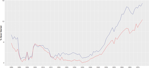
For both men and women, the proportion of never-married individuals decreased from the 1890 to 1899 birth cohorts, increased for the 1905 to 1910 birth cohorts, decreased again until 1915, remained at about the same level with some fluctuations until 1940, and then increased until the 1973 birth cohort, reaching about 15% for men and about 12% for women. With the exception of the 1895 to 1910 birth cohorts, the proportion of never-married men has always been higher than that of never-married women. Moreover, the gap between the proportions of never-married men and women widened after 1945 (Figure 1). Since differences in sex ratios are too small to explain this pattern, it may be due to higher remarriage rates for men than for women, leaving more men unmarried. Evidence for this comes from Hopcroft 2021 (Hopcroft, 2021), who uses U.S. census data to show that men with higher incomes are more likely than women to remarry after divorce and may be “snatching” potential marriage partners from men with lower incomes.

Figure 1. Percentage of never-married individuals by birth year cohort. Blue line for men, red line for women.

Men

For men of all birth cohorts, all three explanatory variables in the full mixed model (of ever married regressed on total income, education, and dwelling ownership) are significantly positively associated with ever married. By far the most variance is explained by total income (6.19%), followed by homeownership (1.0%) and education (0.54%). The random factors year of birth and race together explain 2.82% (2.3% year of birth, 0.52% race) of the total variance in ever married. The sex ratio for each birth year is significantly negatively associated with ever married, but the sex ratio explains only 0.21% of the variance; thus, the course of the time series of ever married is only partially explained by the sex ratio for each birth year. Moreover, both the evolution of the sex ratio and the evolution of the percentage of never-married men by birth year show a substantially different pattern (Supplementary Figure S1). When education is omitted from the model, the estimates change only at the third decimal place Table 1.

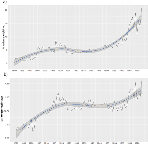
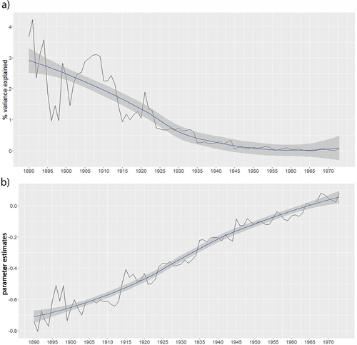
Looking at birth cohorts separately, the variance of ever married explained by total income rises sharply, especially after the 1945 birth cohort. While total income explains only 2.5% of ever married for men born in 1890, the share of variance explained by total income rises to more than 20% for men born in 1973; based on the Loess smoother, the values rise from just over 0% to 17.5% (Figure 2a). For each year of birth, the association between total income and ever married remains positive throughout the time series (Figure 2b). The time series of the regression estimates for total income how much the same pattern, but with a steeper rise from the 1890 to 1920 birth cohorts, followed by a trough and a rise again from 1945 onwards (Figure 2b). Both the variance explained by total income and the regression estimates indicate that, for men, income became increasingly important for ever being married over the time series from 1890 to 1973.

Figure 2. a) Men: Time series of the variance of ever married explained by total income (in %) by birth year cohort. b) Time series of the corresponding regression estimates. Original time series (black line) and loess smoother with confidence intervals.

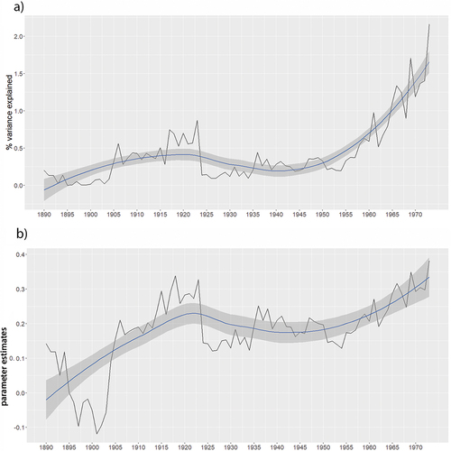
The pattern is very similar for the variance explained by education, but lower by a factor of about 10 (Figure 3a). Again, the values range from almost 0% variance explained for men born in 1890 to 2.2% for men born in 1973 (Figure 3a). The variance explained by education increases until about 1920, then enters a local “valley” and increases again from the birth cohort of about 1942. For each birth year, the estimates of the association between education and having ever been married are positive, except between 1896 and 1903, and rise again until 1920, followed by a trough and a further rise from about 1945 (Figure 3b). In this sense, the pattern of estimates is somewhat similar to that of the variance explained by education (see Figure 3a,b).

Figure 3. 3a) Men: Time series of the variance of ever married explained by education (in %) by birth year cohort. b) Time series of the corresponding regression estimates. Original time series (black line), loess smoother with confidence intervals.

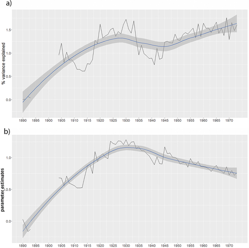
The time series of the variance explained of ever married by dwelling ownership for men shows a steep increase from the birth years 1890 to 1917 and a smaller increase after 1945 (Figure 4a). This suggests that home ownership became more important for ever-marrying over time. Note that data are missing for the birth cohorts from 1893 to 1903. With the exception of the 1890–1892 birth cohorts, the regression estimates of homeownership remain positive throughout the time series, but in contrast to the variance explained, they slowly decline after 1930 (Figure 4b).

Figure 4. a) Men: Time series of the variance of ever-married explained by homeownership (in %) by birth year cohort. b) Time series of the corresponding regression estimates. Original time series (black line), loess smoother with confidence intervals. Data are missing for the birth years 1893–1913.

The results also show that for men, the variance of ever married explained by race fluctuates over the time series, but only occasionally explains more than 2% of the total variance; we cannot explain the outlier between 1905 and 1911 (Supplementary Figure S3a).

Women

For women, with the exception of home ownership, the picture is reversed. Based on the entire data set, total income and education are significantly negatively associated with ever married, while home ownership shows a significant positive association with ever married (Table 2). Overall, the variance explained by each of the three explanatory factors is much lower than for men, especially for total income (0.04% compared to 6.19% for men). The variance of ever married explained by education is 0.19% (compared to 0.54% for men) and that of home ownership is 0.59% (1% for men). The positive associations and the variance explained by the random factors year of birth and race are similar to those found for men (year of birth 0.87%, race 1.8%) (Table 2). Also as for men, sex ratio for each birth year is negatively but only marginally significantly associated with ever married, explaining only 0.091% of the variance. As with men, omitting education from the model only changes the estimates at the third decimal place.

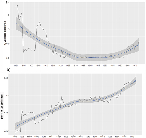
The relationship between income and ever-marrying is reversed for women compared to men, which is also evident when analyzing birth cohorts separately. With the exception of birth cohorts starting in 1964, the association between total income and ever married among women is always negative throughout the time series. This indicates that women with higher incomes have a lower probability of ever being married (Figure 5b). Moreover, not only is the variance explained by total income lower for women than for men over the entire time series (birth years 1890 to 1973), but the time series proceeds in the opposite direction: the variance explained is highest for women born close to 1890 and almost zero for those born in 1973 (Figure 5a).

Figure 5. a) Women: Time series of the variance of ever married explained by income (in %) by birth year cohort. b) Time series of the corresponding regression estimates. Original time series (black line), loess smoother with confidence intervals.

Similarly, the association between ever married and education for women is always negative until the 1960 birth cohort, after which it increases to positive estimates (Figure 6b). Similarly to income, the share of variance explained by education declines until 1955 and then more or less levels off, with a slight increase toward the end (Figure 6a).

Figure 6. a) Women: Time series of the variance of ever married explained by education (in %) by birth year cohort. b) Time series of the corresponding regression estimates. Original time series (black line), loess smoother with confidence intervals.

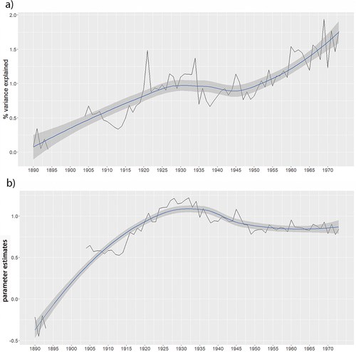
In contrast to the association with income and education, the association between ever married and home ownership is quite similar for men and women. As for men, the variance of ever married explained by home ownership increases from birth years 1890 to 1973 (Figure 7a). The regression estimates of homeownership also show a similar pattern over time for both women and men, with negative values only at the beginning of the time series (Figure 7b).

Figure 7. a) Women: Time series of the variance of ever married explained by home ownership (in %) by birth year cohort. b) Time series of the corresponding regression estimates. Original time series (black line), loess smoother with confidence intervals. Data are missing for birth years 1893–1913.

For women, race generally explains more of the variance in ever married than for men, with a peak at the beginning of the time series, a low around 1939, and a steady increase thereafter (Supplementary Figure S3b).

Discussion

The proportion of never-married men and women is the same for those born between 1895 and 1910. In each of the later birth cohorts, however, more men than women remain unmarried, and the gap widens from the 1945 birth cohort onwards. The average sex ratio at birth over the time series is rather balanced, with only a small overhang of males (about 1059 male births per 1000 female births (https://www.cdc.gov/nchs/pressroom/05facts/moreboys.htm). Thus, the increasing and substantially higher proportion of never-married men compared to women, especially in the later birth cohorts, cannot be explained by an unequal sex ratio at birth. It rather reflects asymmetries in the recruitment into marriage between men and women. Specifically, since the male overhang in the general sex ratio is not large enough to explain the higher proportion of never-married men compared to never-married women, we assume that more men than women have been married more than once, leaving a higher proportion of men unmarried. Following Hopcroft 2021 (Hopcroft, 2021), we further assume that men with higher incomes in particular may remarry more frequently, leaving fewer mating opportunities for men with lower incomes, a pattern that is also consistent with the assumptions of Bateman (Bateman 1948). Unfortunately, our data do not include individual remarriage rates. Thus, we are unable to prove or disprove this claim.

Also, in European countries, preliminary data (see Supplement Fig. 4a-g) suggest that, similar to our results, the proportion of never-married men relative to women increases over time in most countries. In the older cohorts, however, the proportion of never-married women exceeds that of never-married men, probably due to a lower sex ratio at the beginning of the time series, presumably caused by the First and Second World Wars. Koropecki-Cox and Call (Koropeckyj-Cox and Call 2007), using cross-cohort samples from several societies (Australia, Finland, Germany, Japan, the Netherlands, the United Kingdom, and the United States) that included only older cohorts, also reported that men were more likely to be married than women. The discrepancy with our results may be explained by cohort effects, as in our sample the excess of never-married men over never-married women was much smaller in the older cohorts, although the proportion of never-married women never exceeded the proportion of never-married men. We suggest that the surplus of never-married men in the second half of the twentieth century may be explained to some extent by economic development and an increase in inequality. Indeed, in several countries, inequality as measured by the GINI coefficient has increased (Hasell, Morelli, and Roser 2019), which would support the view that income may have become more important for women’s mate choice. However, based on our data, this must remain speculation for now.

Our data are consistent with the notion that the widening gap between the proportions of men and women who never married over time is explained by the increasing pressure on men to earn high incomes in order to find a mate. For men born in 1890, about 2.5 percent of the variance in ever-married status is explained by their respective total earnings; this variance gradually increases to more than 20 percent, especially for birth cohorts from 1945 onward, a time frame that fits well with the widening gap in the proportion of never-married men and women. Importantly, the opposite is found for women: at the beginning of the time series, the effect of income on ever-married is negative, becoming positive only in the most recent cohorts, but then explaining almost nothing of the variance in ever-married.

Although the time series analyzed is far too small to permit definitive conclusions about selection from an evolutionary perspective, this drastic increase in the importance of income for men’s ever-marrying suggests a recent and increasing selection pressure on men exerted by income. This interpretation is supported by studies showing that among men, income predicts ever being married, and marriage predicts ever reproducing (Fieder and Huber 2007, 2022),(Hopcroft, 2021) (Hopcroft 2015)., Thus, income could be viewed as a recent but profound selection pressure on contemporary U.S. men. Although it could be argued that reverse causality may be at work (i.e., ever-married men have higher incomes because they are more ambitious once married), the patterns of divorce and remarriage found by Hopcroft (Hopcroft, 2021) do not support such reverse causality. Moreover, preliminary data suggest that an increase in income increases a man’s chances of marrying shortly thereafter (Huber & Fieder unpublished data).

The time series of the association between education and ever-married among men is similar to that between income and ever-married, although the explained variance is about a factor of 10 lower. Similar to income, education is positively associated with ever married among men (except for the 1896–1903 birth cohorts). In addition, education is increasingly positively associated with income over the time series, with a steep increase up to the 1930 birth cohort and a further slight increase from the 1950 birth cohort onwards (Supplementary Figure S2a). The intermediate flattening of the positive association between education and income may reflect the economic crisis following the Great Depression of the 1930s and the Second World War. However, education explains only a small fraction of the variance in ever-married among men and can thus be considered more as a prerequisite for social status than as a robust status indicator like income (Fieder and Huber 2022), even if education gains in importance over the time series. Education has a substantial hereditary component (~40%) (Bates, 2008) (Branigan, McCallum, and Freese 2013; Engzell and Tropf 2019), and may thus be more indicative of “general cognitive ability” (Plomin and Von Stumm 2018; von Stumm and Plomin 2021) than of status per se, and thus possibly signal the chances of earning a high income. Indeed, a very recent finding shows that increased childlessness among men is mediated by traits such as fluid intelligence, income, and education, with men low on these traits less likely to find a mate and reproduce (Gardner et al. 2022; Kolk and Barclay 2021) also found in a Swedish sample that both low income and low cognitive ability independently predicted low fertility and high childlessness among men. They further found that the main reason for the observed lower fertility among men with lower cognitive ability is their failure to find a partner for a stable union for childbearing.

For women, the effect of income on ever-married turns from negative to positive, but explains less of the variance in ever-married and virtually none of the variance in the most recent cohorts. The time series of the variance in ever married explained by women’s education is similar to that explained by income, with a decline until the 1960 birth cohort and a slight increase thereafter (Figure 6a). Overall, however, education explains little of the total variance. In addition, the sign of the association between ever married and education for women is negative until the 1961 birth cohort (Supplementary Figure 6b). The overall correlation between education and income is lower for women than for men (see Figures S2a,b), increases slightly until about the 1930 birth cohort, increases more steeply until about the 1955 birth cohort, and then flattens out (Supplementary Figure S2b). Thus, education pays off less in terms of income for women than for men, which may be due to the problems women face in reconciling family and work.

For both sexes, home ownership is positively associated with having ever been married for most of the study period, with a peak in the 1931 birth year. However, the variance explained by home ownership is no more than 1.5%, despite a steady increase until the end of the time series. Thus, compared to income, home ownership explains only a small fraction of the variance of ever married. Caution should be exercised in interpretation and causality, as home ownership may increase the probability of marriage, but marriage may also induce investment in home ownership. The time series of home ownership is quite similar for men and women, probably because home ownership is not measured as an individual characteristic but as a household characteristic.

Although cohabitation may have played a less important role than marriage, since marriage was prevalent for most of the time series examined and most children in the US were born within marriages throughout the period considered, we also examined recent patterns of cohabitation and found comparable results, which are presented in the Supplement (Supplement Cohabitation in the US).

We have no explanation yet, why the random factor race explains more of the variance in ever being married among women.

Our results allow only speculation about possible “evolutionary forces,” but suggest that income exerts a recent but substantial selective pressure on men to find a mate and thus reproduce. In contrast, for women there was, if anything, a negative selection pressure from income, which disappeared in the cohorts born after 1945. Social status has been very important for men to find a mate and reproduce throughout human history. This ranges from traditional societies (Borgerhoff Mulder 1988; Chagnon 1988; Cronk 1989; Irons 1979; Mealey 1985; Voland 1990; Von Rueden, Gurven, and Kaplan 2008) to industrial societies (Fieder and Huber 2007; Fieder et al. 2005; Fieder, Huber, and Bookstein 2011; Hopcroft 2006, 2015; Nettle and Pollet 2008; Weeden et al. 2006),(Barthold et al., 2012). Similarly, a meta-analysis by (Von Rueden and Jaeggi 2016) based on 288 outcomes from 33 nonindustrial populations shows that, overall, male social status is significantly positively associated with male reproductive success. In these 33 nonindustrial populations, regardless of how status is defined and how status is actually measured, it is an important characteristic for male reproduction in particular. Nevertheless, over the course of the 20th and early 21st centuries, what counts as “social status” has apparently become increasingly narrow, with income appearing to outperform all other male status indicators as a mate selection criterion. Indeed, we have recently shown that income outperforms other mate selection criteria such as attractiveness (Fieder and Huber 2022). This is of particular interest because social status has historically been defined differently across societies and circumstances. With income, a globally valid, convertible “measure” of social status has emerged. It can act as a selective force not only in individual populations, but also globally, and thus may represent a historically unprecedented, broad selective force.

(Buss et al. 2001) showed that the importance of good financial prospects in a potential marriage partner is increasing for both men and women, although this trend is stronger for men than for women, thereby reducing the gender difference in the importance of good financial prospects in a potential spouse. These changes in preferences may be the result of changes in women’s participation in the labor force, leading to higher incomes and financial independence for women. However, these preferences found by Buss et al. (2001) do not manifest themselves in actual marriage patterns, as our data show, on the contrary, that the importance of income has increased over time for male, but not for female, marriage partners. Thus, despite women’s greater financial independence, the importance of their spouse’s income has increased rather than decreased. Our data suggest that as women’s education and income increase, so do their demands for education and income in a potential spouse, a trend that leads to greater pressure on men to earn higher incomes.

Beyond speculation about evolutionary outcomes, however, we must also consider that the social consequences of the patterns described may be very problematic. For example, the incel (involuntary celibacy (https://www.theglobeandmail.com/canada/article-the-incel-community-and-the-dark-side-of-the-internet/ (Hoffman, Ware, and Shapiro 2020; O’Malley, Holt, and Holt 2020); movement that has emerged over the past 20 years or so may be a consequence of the increasing proportion of never-married men and the increasing pressure on men to earn high incomes in order to find a mate. Indeed, using Twitter data (Brooks, Russo-Batterham, and Blake 2022), found that incel-related tweets are more common in places where mating competition among men is high due to male-biased sex ratios, few single women, high income inequality, and small gender gaps in income. The more important a man’s income is to a woman’s mating decision, the higher the proportion of men who are “left behind” and never find a mate, with all the social and political consequences that can disrupt societies. Thus, the number of “left-behind men” may also have increased due to rising inequality in the US and also in some European countries (Hasell, Morelli, and Roser 2019).

Acknowledgments

Steven Ruggles, Sarah Flood, Ronald Goeken, Megan Schouweiler and Matthew Sobek. IPUMS USA: Version 12.0 [dataset]. Minneapolis, MN: IPUMS, 2022. https://doi.org/10.18128/D010.V12.0

Steven Ruggles, Catherine A. Fitch, Ronald Goeken, J. David Hacker, Matt A. Nelson, Evan Roberts, Megan Schouweiler, and Matthew Sobek. IPUMS Ancestry Full Count Data: Version 3.0 [dataset]. Minneapolis, MN: IPUMS, 2021.

Disclosure statement

No potential conflict of interest was reported by the author(s).

Supplemental data

Supplemental data for this article can be accessed online at https://doi.org/10.1080/19485565.2023.2220950

Additional information

Funding

The author(s) reported there is no funding associated with the work featured in this article.

References

- Bateman, A. J. 1948. Intra-sexual selection in Drosophila. Heredity 2 (3):349–68. doi:10.1038/hdy.1948.21.
- Betzig, L. L. 1986. Despotism and differential reproduction: A Darwinian view of history. Milton Park, UK: Aldine Publishing Co.
- Barthold, J. A., Myrskylä, M., & Jones, O. R. 2012. Childlessness drives the sex difference in the association between income and reproductive success of modern Europeans. Evolution and Human Behavior, 33 (6): 628-638.
- Borgerhoff Mulder, M. 1988. Reproductive success in three Kipsigis cohorts. In Reproductive Success, 419–38. Chicago: Univ. Chicago Press.
- Branigan, A. R., K. J. McCallum, and J. Freese. 2013. Variation in the heritability of educational attainment: An international meta-analysis. Social Forces 92 (1):109–40.
- Brooks, R. C., D. Russo-Batterham, and K. R. Blake. 2022. Incel activity on social media linked to local mating ecology. Psychological Science 33 (2):249–58. doi:10.1177/09567976211036065.
- Brzozowska, Z., E. Beaujouan, and K. Zeman. 2022. Is two still best? Change in parity-specific fertility across education in low-fertility countries. Population Research and Policy Review 41 (5):2085–114. doi:10.1007/s11113-022-09716-4.
- Bulanda, J. R., and S. L. Brown. 2007. Race-ethnic differences in marital quality and divorce. Social Science Research 36 (3):945–67. doi:10.1016/j.ssresearch.2006.04.001.
- Buss, D. M., T. K. Shackelford, L. A. Kirkpatrick, and R. J. Larsen. 2001. A half century of mate preferences: the cultural evolution of values. Journal of Marriage & Family 63 (2):491–503.
- Chagnon, N. A. 1988. Life histories, blood revenge, and warfare in a tribal population. Science 239 (4843):985–92. doi:10.1126/science.239.4843.985.
- Clark, G. 2008. A farewell to alms. Princeton University Press. doi: 10.1515/9781400827817.
- Cronk, L. 1989. Low socioeconomic status and female‐biased parental investment: the Mukogodo example. American Anthropologist 91 (2):414–29. doi:10.1525/aa.1989.91.2.02a00090.
- Engzell, P., and F. C. Tropf. 2019. Heritability of education rises with intergenerational mobility. Proceedings of the National Academy of Sciences 116 (51):25386–88. doi:10.1073/pnas.1912998116.
- Fieder, M., and S. Huber. 2007. The effects of sex and childlessness on the association between status and reproductive output in modern society. Evolution and Human Behavior 28 (6):392–98. doi:10.1016/j.evolhumbehav.2007.05.004.
- Fieder, M., and S. Huber. 2020. Effects of wife’s and husband’s income on wife’s reproduction: An evolutionary perspective on human mating. Biodemography and Social Biology 65 (1):31–40. doi:10.1080/19485565.2019.1689351.
- Fieder, M., and S. Huber. 2022. Contemporary selection pressures in modern societies? Which factors best explain variance in human reproduction and mating?. Evolution and Human Behavior 43 (1):16–25. doi:10.1016/j.evolhumbehav.2021.08.001.
- Fieder, M., S. Huber, and F. L. Bookstein. 2011. Socioeconomic status, marital status and childlessness in men and women: An analysis of census data from six countries. Journal of Biosocial Science 43 (5):619–35. doi:10.1017/S002193201100023X.
- Fieder, M., S. Huber, F. L. Bookstein, K. Iber, K. Schäfer, G. Winckler, and B. Wallner. 2005. Status and reproduction in humans: new evidence for the validity of evolutionary explanations on basis of a university sample. Ethology 111 (10):940–50. doi:10.1111/j.1439-0310.2005.01129.x.
- Gardner, E. J., M. D. Neville, K. E. Samocha, K. Barclay, M. Kolk, M. E. Niemi, G. Kirov, H. C. Martin, and M. E. Hurles. 2022. Reduced reproductive success is associated with selective constraint on human genes. Nature 603 (7903):858–63. doi:10.1038/s41586-022-04549-9.
- Goldin, C. 2021. Career and family. Career and Family, Princeton University Press. 10.1515/9780691226736
- Goodman, A., and I. Koupil. 2010. The effect of school performance upon marriage and long-term reproductive success in 10,000 Swedish males and females born 1915–1929. Evolution and Human Behavior 31 (6):425–35. doi:10.1016/j.evolhumbehav.2010.06.002.
- Goodwin, P. 2009. Who Marries and When?: Age at First Marriage in the United States, 2002. Atlanta: US Department of Health and Human Services, Centers for Disease Control and. 19.
- Gurven, M., and C. Von Rueden. 2006. Hunting, social status and biological fitness. Biodemography and Social Biology 53 (1–2):81–99. doi:10.1080/19485565.2006.9989118.
- Guzzo, K. B., and S. R. Hayford. 2020. Pathways to parenthood in social and family contexts: decade in review, 2020. Journal of Marriage & Family 82 (1):117–44. doi:10.1111/jomf.12618.
- Hackman, J., and D. Hruschka. 2020. Disentangling wealth effects on fertility in 64 low-and middle-income countries. Evolutionary Human Sciences 2:e58. doi:10.1017/ehs.2020.62.
- Hasell, J., S. Morelli, and M. Roser. 2019. Recent trends in educing social inequalities in cancer: evidence and priorities for research, International Agency for Research on Cancer. Eds.: Vaccarella S, Lortet-Tieulent J, Saracci R., 2019, Lyon, France.
- Hawkes, K. 2019. Why do men hunt? Benefits for risky choices. In Risk and uncertainty in tribal and peasant economies, 145–66. Milton Park, UK: Routledge.
- Hoffman, B., J. Ware, and E. Shapiro. 2020. Assessing the threat of incel violence. Studies in Conflict & Terrorism 43 (7):565–87. doi:10.1080/1057610X.2020.1751459.
- Hopcroft, R. L. 2006. Sex, status, and reproductive success in the contemporary United States. Evolution and Human Behavior 27 (2):104–20. doi:10.1016/j.evolhumbehav.2005.07.004.
- Hopcroft, R. L. 2015. Sex differences in the relationship between status and number of offspring in the contemporary US. Evolution and Human Behavior 36 (2):146–51. doi:10.1016/j.evolhumbehav.2014.10.003.
- Hopcroft, R. L. 2021. High income men have high value as long-term mates in the US: Personal income and the probability of marriage, divorce, and childbearing in the US. Evolution and Human Behavior 42 (5):409–17. doi:10.1016/j.evolhumbehav.2021.03.004.
- Huber, S., F. L. Bookstein, and M. Fieder. 2010. Socioeconomic status, education, and reproduction in modern women: an evolutionary perspective. American Journal of Human Biology 22 (5):578–87. doi:10.1002/ajhb.21048.
- Irons, W. 1979. Natural selection, adaptation, and human social behavior. In Eds: N. Chagnon & W. Irons Evolutionary Biology and Human Behavior, 4–39. Duxbury, Boston, MA
- Jalovaara, M., G. Neyer, G. Andersson, J. Dahlberg, L. Dommermuth, P. Fallesen, and T. Lappegård. 2019. Education, gender, and cohort fertility in the Nordic countries. European Journal of Population 35 (3):563–86. doi:10.1007/s10680-018-9492-2.
- Kolk, M. 2022. The relationship between life-course accumulated income and childbearing of Swedish men and women born 1940–70. Population Studies 1–19. doi:10.1080/00324728.2022.2134578.
- Kolk, M., and K. Barclay. 2021. Do income and marriage mediate the relationship between cognitive ability and fertility? Data from Swedish taxation and conscriptions registers for men born 1951–1967. Intelligence 84:101514. doi:10.1016/j.intell.2020.101514.
- Koropeckyj-Cox, T., and V. R. Call. 2007. Characteristics of older childless persons and parents: cross-national comparisons. Journal of Family Issues 28 (10):1362–414. doi:10.1177/0192513X07303837.
- McIntosh, B., R. McQuaid, A. Munro, and P. Dabir‐Alai. 2012. Motherhood and its impact on career progression. Gender in Management: An International Journal 27 (5):346–64. doi:10.1108/17542411211252651.
- Mealey, L. 1985. The relationship between social status and biological success: A case study of the Mormon religious hierarchy. Ethology and Sociobiology 6 (4):249–57. doi:10.1016/0162-3095(85)90017-2.
- Nakagawa, S., P. C. Johnson, and H. Schielzeth. 2017. The coefficient of determination R 2 and intra-class correlation coefficient from generalized linear mixed-effects models revisited and expanded. Journal of the Royal Society Interface 14 (134):20170213. doi:10.1098/rsif.2017.0213.
- Nakagawa, S., H. Schielzeth, and R. B. O’Hara. 2013. A general and simple method for obtaining R2 from generalized linear mixed-effects models. Methods in Ecology and Evolution 4 (2):133–42. doi:10.1111/j.2041-210x.2012.00261.x.
- Nettle, D., and T. V. Pollet. 2008. Natural selection on male wealth in humans. The American Naturalist 172 (5):658–66. doi:10.1086/591690.
- Nisén, J., P. Martikainen, M. Myrskylä, and K. Silventoinen. 2018. Education, other socioeconomic characteristics across the life course, and fertility among Finnish men. European Journal of Population 34 (3):337–66. doi:10.1007/s10680-017-9430-8.
- Nisén, J., P. Martikainen, K. Silventoinen, and M. Myrskylä. 2014. Age-specific fertility by educational level in the Finnish male cohort born 1940–1950. Demographic Research 31:119–36. doi:10.4054/DemRes.2014.31.5.
- O’Malley, R. L., K. Holt, and T. J. Holt. 2020. An exploration of the involuntary celibate (incel) subculture online. Journal of Interpersonal Violence 37 (7–8):NP4981–NP5008. doi:10.1177/0886260520959625.
- Plomin, R., and S. Von Stumm. 2018. The new genetics of intelligence. Nature Reviews Genetics 19 (3):148–59. doi:10.1038/nrg.2017.104.
- Stearns, S. C., S. G. Byars, D. R. Govindaraju, and D. Ewbank. 2010. Measuring selection in contemporary human populations. Nature Reviews Genetics 11 (9):611–22. doi:10.1038/nrg2831.
- Steven Ruggles, Sarah Flood, Matthew Sobek, Danika Brockman, Grace Cooper, Stephanie Richards, and Megan Schouweiler. 2023. IPUMS USA: Version 13.0 [dataset]. Minneapolis, MN: IPUMS. doi:10.18128/D010.V13.0.
- Stulp, G., M. J. Simons, S. Grasman, and T. V. Pollet. 2017. Assortative mating for human height: A meta‐analysis. American Journal of Human Biology 29 (1):e22917. doi:10.1002/ajhb.22917.
- Torr, B. M. 2011. The changing relationship between education and marriage in the United States, 1940–2000. Journal of Family History 36 (4):483–503. doi:10.1177/0363199011416760.
- Voland, E. 1990. Differential reproductive success within the Krummhörn population (Germany, 18th and 19th centuries). Behavioral Ecology and Sociobiology 26 (1):65–72. doi:10.1007/BF00174026.
- Von Rueden, C., M. Gurven, and H. Kaplan. 2008. The multiple dimensions of male social status in an Amazonian society. Evolution and Human Behavior 29 (6):402–15. doi:10.1016/j.evolhumbehav.2008.05.001.
- Von Rueden, C., M. Gurven, and H. Kaplan. 2011. Why do men seek status? Fitness payoffs to dominance and prestige. Proceedings of the Royal Society B: Biological Sciences 278 (1715):2223–32. doi:10.1098/rspb.2010.2145.
- Von Rueden, C. R., and A. V. Jaeggi. 2016. Men’s status and reproductive success in 33 nonindustrial societies: Effects of subsistence, marriage system, and reproductive strategy. Proceedings of the National Academy of Sciences 113 (39):10824–29. doi:10.1073/pnas.1606800113.
- von Stumm, S., and R. Plomin. 2021. Using DNA to predict intelligence. Intelligence 86:101530. doi:10.1016/j.intell.2021.101530.
- Weeden, J., M. J. Abrams, M. C. Green, and J. Sabini. 2006. Do high-status people really have fewer children?. Human Nature 17 (4):377–92. doi:10.1007/s12110-006-1001-3.
- Zhang, Y., and P. Santtila. 2022. Social status predicts different mating and reproductive success for men and women in China: Evidence from the 2010–2017 CGSS data. Behavioral Ecology and Sociobiology 76 (7):101. doi:10.1007/s00265-022-03209-2.