Numerical investigation of interfacial mass transfer in two phase flows using the VOF method

ABSTRACT

A mass transfer model is developed using the volume-of-fluid (VOF) method with a piecewise linear interface calculation (PLIC) scheme in ANSYS FLUENT for a free-rising bubble. The mass flow rate is defined via the interface by Fick's law and added into the species equation as a source term in the liquid phase using the user-defined functions (UDFs) in ANSYS FLUENT. The interfacial concentration field for the mass flow rate is discretized by two numerical methods. One of them is based on the calculation of the discretization length between the centroid of the liquid volume and the interface using the liquid void fraction and interface normal vectors at the interface cells, while in the second method the discretization length is approximated using only the liquid void fraction at the interface cells. The influence of mesh size, schemes, and different Schmidt numbers on the mass transfer mechanism is numerically investigated for a free-rising bubble. Comparison of the developed mass transfer model with the theoretical results shows reasonable and consistent results with a smaller time-step size and with cell size.

KEYWORDS:

• interfacial mass transfer
• VOF method
• free-rising bubble

Nomenclature

Roman Symbols
A	=	Interfacial area (m2)
d	=	Diameter (m)
k	=	Mass transfer coefficient (m/s)
a	=	Mesh scale (m)
	=	Mass transfer rate (kg/s)
N	=	Number of mesh cells (–)
S	=	Source term (kg/m3 s)
U	=	Velocity (m/s)
V	=	Volume (m3)

Greek Symbols

	=	Discretization length at the interface cells (m)
	=	Rate of energy dissipation per unit mass viscosity (m3/s2)
	=	Void fraction (–)
	=	Pi number (–)

Subscripts

0	=	Initial
avg	=	Average
bat	=	Batchelor
bub	=	Bubble
dis	=	Dissolution
int	=	Interface
Kol	=	Kolmogorov
l	=	Liquid phase
g	=	Gas phase
norm	=	Normalized
sat	=	Saturation
x	=	Cell index in x direction
y	=	Cell index in y direction
z	=	Cell index in z direction

Acronyms

Re	=	Reynolds number
Pe	=	Peclet Number
Sc	=	Schmidt number
Gr	=	Grashof number

1. Introduction

Micro process engineering offers the advantage of fast heat removal and considerable increase in mass transfer through a high gas–liquid interfacial area in continuous operation. The description of the interfacial mass transfer rate between the gas and liquid phases is necessary to predict the degree of process intensification. In order to optimize the process conditions and reactor geometry, a detailed understanding of the mass transfer process is essential. A combination of the shortcomings of micro scale measurement techniques and the advantages of computational fluid dynamics (CFD) code to visualize, for example, concentration profiles encourages the usage and improvement of CFD research and tools. A trend in the CFD field is to model gas/liquid and liquid/liquid systems in the systems using commercial CFD code and in-house CFD code based on the volume-of-fluid (VOF) method for process development and intensification (Kreutzer, Kapteijn, Moulijna, & Heiszwolf, 2005; Qian & Lawal, 2006). Nowadays commercial CFD code can capture the interface between two immiscible phases (Özkan, Wörner, Wenka, & Soyhan, 2007). The VOF method gives consistent results in experimental research (Ozmen-Cagatay & Kocaman, 2011; Wang, Su, Wang, Zhu, & Liu, 2014). The implementation of interfacial mass transfer with coupled mass balance to provide gas volume shrinkage and the implementation of chemical reactions in multiphase systems are missing or under development. However, this is necessary to understand the effects occurring due to mass transfer between the dispersed phase and continuous phase and to describe the yield and selectivity of chemical reactions in micro-structured devices (Kröger, Alke, Bothe, & Warnecke, 2007).

In the present research we have focused on the discretization of the local mass transfer equation through the application of Fick's law using two numerical concepts in ANSYS FLUENT (ANSYS, 2009). Since ANSYS FLUENT offers the usage of mass transfer source term using the VOF method and the piecewise linear interface calculation (PLIC) scheme, it is possible to add the interfacial mass transfer based on the concentration difference via user-defined functions (UDFs). Therefore, like the study of Sato, Jung, and Abe (2000) we set the saturation concentration at the interface cells as a boundary condition. The VOF method with the PLIC scheme is based on a generalization of the method of Youngs (1982) can be considered in ANSYS Fluent as one of the most accurate scheme to calculate the void fraction (ANSYS, 2009). The standard multiphase species equation is used in ANSYS FLUENT to get the dissolution concentration in the liquid phase. In order to integrate a mass source based on Fick's law at the interface cells, the discretization liquid length (the distance between the interface and the centroid of the liquid volume) must be calculated. We applied two different numerical concepts. One is based on the calculation of discretization length between the centroid of the liquid volume and the interface using the liquid void fraction and the interface normal vectors delivered from the VOF–PLIC scheme, while in the other the discretization length is approximated using only the liquid void fraction at the interface cells. By applying these concepts it is possible to directly link mass transfer with the bubble volume change. In all simulations, ANSYS FLUENT version 12 was used. In order to implement interfacial mass transfer, the define mass transfer (DMT) macro was used for the calculation of the relevant source terms.

2. Calculation of

UDFs allow users to modify the behavior of ANSYS FLUENT in order to meet their specific modeling needs. The interfacial mass transfer model based on Fick's law is implemented using the DMT macro in the VOF–PLIC model with species transport equations. Multiphase species transport equation is taken account of at the liquid phase cells in the macro (0<al≤1) since the internal mass transfer in the bubble is not considered in the present research. More detail about the methodology is available in the ANSYS FLUENT theory guide (ANSYS, 2009).

is the mass transfer from the gas phase to the liquid phase. Since mass transfer from liquid to gas is not considered, is not accounted for and therefore the source term (S) is: (1) where is the interfacial mass transfer source between species O₂ in air and the liquid mixture from gas phase to liquid phase. It can be calculated by Fick's first law as: (2) where A is the interfacial area and it can be calculated for each cell by multiplying the cell volume and the magnitude of the void fraction gradient (Wielage, 2005): (3)

The derivation of the gas void fraction () in the x, y, z direction is 0 except at the interface cells. This restriction provides the selection of interface cells since S is 0 except at the interface cells.

For the gas volume fraction in the cell, , the following three conditions are possible:

 = 0: The cell is empty of gas.

 = 1: The cell is full of gas.

0 <  < 1: The cell contains the interface between gas and liquid

The void fraction for the gas phase in terms of the mass transfer is (4)

Calculation of at the interface cells is achieved as long as the void fraction of the liquid phase is greater than .05 to keep the convergence. Otherwise the concentration gradient approaches infinity, since the discretization length approaches zero without the liquid void fraction restriction. The gradient of concentration in Equation (2) is calculated by (5) where is the saturation concentration and set by the user, is the dissolution concentration in the liquid phase, and finally is the missing discretization length. is normally stored at the center of the mesh cell but it is assumed that it is at the center of gravity of the cut liquid volume. The determination of is based on the two alternative numerical concepts presented in Figure 3.

Figure 1. A typical 3D uniform cubic mesh cell (left), and 2D uniform quadratic mesh cells for the mesh refinement strategy (right).

Figure 2. A cross-section of the computational domain at z = 8 mm in 3D (left) and 2D (right).

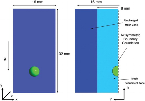
Figure 3. 2D schematic of interface cells and calculation of based on the PLIC-1 and PLIC-2 methods.

Figure 4. Flowchart for calculating in the PLIC method.

The local void fraction of liquid and normal vectors at the interface are required in order to calculate (for the PLIC-1 method). The VOF method using the PLIC scheme delivers this information. Therefore, the numerical concept of the PLIC-1 calculation of is more accurate. In the concept of the PLIC-2 method, only the void fraction equation is used from the PLIC scheme. However, in order to calculate from the void fraction value, it is assumed that the interface is parallel to a certain interface cell (in contrast to the PLIC scheme itself). The discretization length in Equation (5) is thus approximated.

In the PLIC-1 method the normal vectors of the interface and the -value are provided from the ANSYS FLUENT code to calculate . Figure 4 shows the flowchart of the calculation. More detail about mathematical calculation method are available in Oezkan (2013). In order to identify the position of the interface in the cells, the code iterates. Starting with an initial point in the middle of the cell, the phase volumes are calculated using the normal vector and this initial point is given as a position of the interface plane (Figure 5). These phase volumes are compared with the -value. If the phase volumes are not consistent with , the position of the plane is changed until this criterion is fulfilled. Then is calculated. Determination of the discretization length is easier in PLIC-2 method; since cubic cells are used, the individual phases are separated into cuboid sections and the normal vector is rectangular to one of the cell walls. Thus can easily be calculated according to the following equation for a unit cell length (a): (6)

Figure 5. Demonstration of iteration in the PLIC-1 method.

3. Results and discussion

The rise of an air bubble in a water system is simulated in order to investigate the implementation of the mass transfer. The oxygen transfer in air is considered for the interfacial mass transfer. The results for mass transfer are compared against the numerical approach published by Bothe, Koebe, Wielage, and Warnecke (2003) and a Sherwood correlation by Chao (1962) and Calderbank and Moo-Young (1961). The approach of Bothe et al. (2003) is applied here for a 1.6 × 3.2 × 1.6·10⁻² m 3D computational domain, discretized with 50 × 100 × 50 uniform cubic mesh cells. In the 3D simulations, the computational domain of Bothe's benchmark was used for the one-to-one comparisons. However, in the 2D simulations, the computational domain is modified to avoid the influence of the wall on the bubble rise velocity. Therefore, the channel diameter in the 2D simulations is increased to 3.2·10⁻² m.

A locally uniform square mesh refinement is provided in the 2D simulations in the center in order to investigate the influence of grid resolution on mass transfer. After the refinement process, the mesh size is 1.6·10⁻⁴ m in the first mesh refinement, 0.8·10⁻⁴ m in the second mesh refinement, and 0.4·10⁻⁴ m in the third mesh refinement for a size of 1.6 × 3.2·10⁻² m (Figures 1 and 2). In order to minimize the difference of the velocity gradient between unchanged mesh cells and mesh refinement cells, the mesh size is reduced step by step.

The bubble is at fluid rest at x,y,z = (8, 8, 8) 10⁻³ m in 3D and h,r = (8, 0) 10⁻³ m in 2D cylindrical coordinates (Figure 2). The initial bubble diameter at these positions should have been 4·10⁻³ m according to Bothe's benchmark. In our calculations, it was possible to initialize the bubble diameter as 3.84·10⁻³ m using the mesh size 3.2·10⁻⁴ m. The four sides and the bottom wall are defined with no-slip boundary conditions, while a boundary condition of pressure outlet is implemented on the top side.

In the present research, the external mass transfer from air into a miscible water–glycerol mixture at 1 bar and room temperature was investigated. The physical properties at 1 bar and room temperature under simulation are listed in Table 1.

Table 1. Physical properties of liquid and gas at 1 bar and room temperature.

Medium	Liquid		Gas
Viscosity (Pa.s)	7.5 × 10^−2		18.24 × 10^−6
Density (kg/m^3)	1205		1.122
Surface tension (N/m)		0.063
Gas diffusivity in liquid (m^2/s)		62.24 × 10^−8
Saturation concentration (kg/m^3)		0.008

The comparisons for volume change are based on a history of normalized diameter () which is calculated as (7) where is the bubble diameter during the free rising and is the initial bubble diameter. Figure 6 shows the progression of the normalized diameter of the bubble due to mass transfer calculated by the PLIC-1 and PLIC-2 methods with a 50 × 100 × 50 cells and uniform mesh. We should note that the results are dependent on the mesh. The influence of the mesh on the 3D calculations is not investigated in this study due to the high CPU time, but it is examined in the 2D simulations. From Figures 6–11 the mesh interval size is 3.2·10⁻⁴ m.

Figure 6. Normalized diameter of the free-rising bubble for the two different calculation methods.

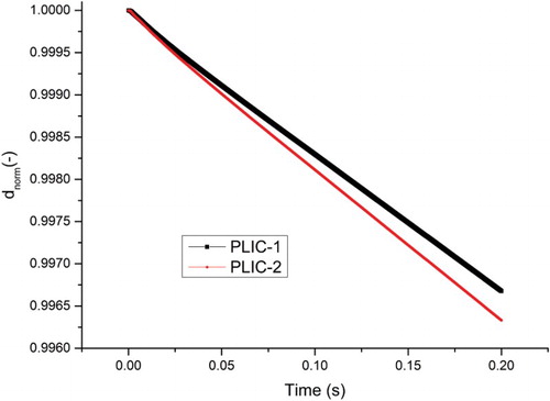
Figure 7. Concentration profile in the flow direction (y-axis) in the middle of the channel using the PLIC-1 and PLIC-2 methods. Note: CWL = concentration wake length of traceable gaseous species in the liquid.

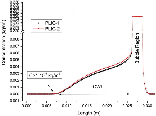
Figure 8. Comparison of the numerical results with the empirical Sherwood correlations.Note: In the numerical results of PLIC-1, the first-order scheme for the momentum and species equation and a 50 × 100 × 50 mesh resolution are used.

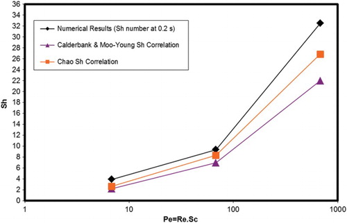
Figure 9. The concentration distribution at Sc = 1 (left), Sc = 10 (middle), and Sc = 100 (right) at 0.2 s. Note: The colored scale represents the concentration of oxygen in kg/m³. In the numerical results of PLIC-1, the first-order scheme for the momentum and species equation and a 50 × 100 × 50 mesh resolution are used.

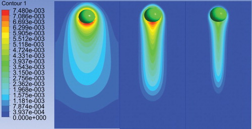
Figure 10. Comparison of the numerical results with empirical Sherwood correlations.

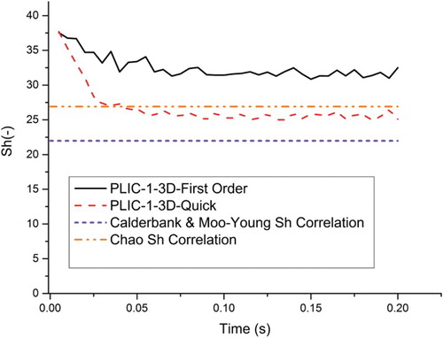
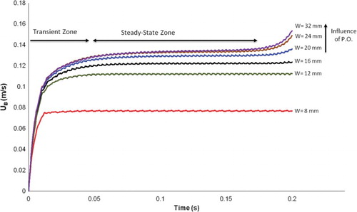
Figure 11. Temporal evolution of bubble velocity for different channel diameters with an interval mesh size of 3.2·10⁻⁴ m in 2D. Note: W = channel diameter.

The concentration profile at the middle line of the computational domain is shown in Figure 7. Calculation of using the same void fractions in cubic cells gives similar results for both methods. PLIC-1 is more accurate but on the other hand the calculation time of in PLIC-2 is fast, since the iteration progress is not needed.

Consistent results are obtained in comparison to results from literature (Bothe et al. 2003; Onea, 2006; Raymond & Rosant, 2000; see Table 2). The bubble aspect ratios and bubble velocities of the different numerical analyses are very near to our results. The hydrodynamic results as well as the aspect ratio of the bubble also show good agreement with the experimental observations of Raymond and Rosant (2000).

Table 2. Comparison of the experimental results with the data in the literature at 0.2 s absorption time.

	Bothe (2003)	Onea (2006)	Raymond (2000)	PLIC-1 results
CWL (m)	0.014	0.018	–	0.018
AR	0.86	0.87	0.86	0.87
Ubub(m/s)	0.12	0.11	0.13	0.11

Note: CWL = concentration wake length of traceable gaseous species in the liquid; AR = aspect ratio of bubble).

There is no available experimental data with which to compare the concentration distributions. One of the difficulties lies in measuring the concentration distribution and values in spatial and time resolution. Investigations of the bubble dissolution in continuous phases are under development. However, in the numerical results, some assumptions are still made, which may produce differences in the experiment; for example, piecewise incompressible fluids, contaminated influence and the Marangoni effect are not considered. Therefore we tried to compare our results with theoretical correlations to prove the models’ under parameter variation.

A well-known Sherwood correlation from Calderbank and Moo-Young (1961) for free-rising bubbles () is (8) where the Grashof (Gr) number is (9)

The Sherwood (Sh) number correlation from Chao (1962) is a function of Re and Sc for bubble spheres with mobile interfaces as follows: (10)

The Reynolds number is calculated according to (11) where d_bub is the diameter of the bubble and U_bub is the bubble velocity calculated by (12) where is the y-component of the velocity in all gas cells, the subscripts x, y and z denote the mesh cell index in the x-,y-, and z-directions, and Nx, Ny and Nz denote the number of mesh cells in these directions within the computational domain. (13)

In order to compare the numerical results with the empirical correlations we altered the diffusion coefficient artificially by a factor of 10 and 100 (corresponding to Sc = 10 and Sc = 1, respectively). Figure 8 shows the Sherwood numbers over the logarithmic Peclet numbers. The numerical Sh results calculated in Figure 8 overestimate the mass transfer calculated from the empirical results.

Figure 9 shows the concentration gradients in the liquid at Re = 7.06 for different Sc numbers. For Sc = 1, a very long concentration wake length and width can be observed. The concentration gradient at Sc = 10 is less in comparison to the concentration gradient at Sc = 1. The concentration length and width is also smaller. In the real physical case (at Sc = 100) the concentration length and width are qualitatively similar to the experimental observations by Francois, Dietrich, Guiraud, and Cock (2011).

In all simulations for the pressure-velocity coupling scheme, the pressure-implicit with splitting of operators (PISO), which is based on a higher degree of approximate relation between the corrections for pressure and velocity, is implemented. The comparison of quadratic upstream interpolation for convective kinetics (QUICK) and first-order schemes for mass and species equations is shown in Figure 10 by plotting the numerical Sherwood number against the bubble rising-time. In first-order schemes quantities at cell faces are determined by assuming that the cell-center values of any field variable represent a cell average value and the face quantities are identical to the cell quantities. For the quadrilateral and hexahedral meshes, ANSYS FLUENT also provides the QUICK scheme for computing a higher-order value of the variable at a face. QUICK-type schemes are based on a weighted average of second-order-upwind and central interpolations of the variable, and give more accurate solutions on structured meshes. From Figure 10 it can be seen that the numerical Sherwood number is high at the beginning of the bubble rise since there is almost no gas concentration in the liquid phase. In the comparison of the schemes, the numerical Sherwood number with QUICK scheme is between the theory of Chao (1962) and the theory of Calderbank and Moo-Young (1961), whereas the first-order scheme overestimates the mass transfer. The QUICK scheme is used in the 2D simulations because of its greater accuracy.

For the geometry of the computational domain, the approach of Bothe et al. (2003) was followed for one-to-one comparison in the 3D simulations. However, the investigations for the influence of wall boundary condition on bubble rise velocity have been done in 2D using an interval mesh size of 3.2·10⁻⁴ m to save CPU time. The diameter of the channel was varied between approximately two and eight times the diameter of the bubble. The line W = 16·10⁻³ m corresponds to the bubble velocity using the benchmark of Bothe et al. (2003) in Figure 11. As the channel diameter increases, so does the bubble rise velocity. The influence of the channel diameter on the bubble velocity minimizes after the channel width reaches six times the bubble diameter and it almost disappears at a channel diameter of 32·10⁻³ m. Interestingly, the bubble velocity at the steady-state zone approaches 0.13 m/s, which is an experimental observation from Raymond and Rosant (2000) (see Table 2). Influence of the pressure outlet on bubble velocity can be observed after 0.17 s when the channel diameter is greater than 16 mm. The bubble velocity at the channel diameter of 8·10⁻³ mm reaches clearly a steady state earlier compared to other bubble velocities at channel diameter bigger than 8·10⁻³ mm. It reaches a steady state earlier. If the channel diameter is greater than 8 mm then the required time in the transient zone increases. Since the channel diameter of 32·10⁻³ m has no influence on the bubble rise velocity, it was selected for the investigation of interfacial mass transfer calculations.

In order to continue the investigations on the influence of the mesh size on mass transfer, we switched to axis-symmetric 2D simulations and implemented the PLIC-1 method. A time-step size (10⁻⁶ s) on mass transfer for the smallest mesh size (4·10⁻³ m) was implemented in all 2D simulations. For momentum and species equations, the QUICK scheme was implemented.

The influence of the mesh size on the Sherwood number is shown in Table 3. The numerical average of the Sherwood number between 0.05 and 0.15 s (in the steady-state zone) is calculated as follows: (14)

Table 3. Influence of grid resolution on mass transfer.

Mesh size (m)	3.2×10^−4	1.6×10^−4	0.8×10^−4	0.4×10^−4
	1.12×10^−9	1.4×10^−9	1.44×10^−9	1.4×10^−9
	3.5×10^−3	4.3×10^−3	4.4×10^−3	4.3×10^−3
	20.1	26.3	27.7	27.2

where n is the number of selected time points and k_avg is the average mass transfer coefficient, defined as (15)

For the direct numerical simulations, the consistency of the minimum-length scale is essential. The Kolmogorov length scale should be used for velocity gradients as its implementation avoids viscosity domination and provides the smallest scales of turbulence. In addition, for the concentration field the Batchelor scale describes the smallest length scales of large fluctuations in concentration before molecular diffusion dominates. Determination of the Batchelor length scale provides a true numerical coupling between the diffusive transport of species equation and the momentum equation (Batchelor, 1959). Therefore, for a precise and direct numeric simulation, the length scale of the unit cell and thus in the interface cell should be in the range of the Kolmogorov and/or Batchelor length scales, which should be considered for the velocity and concentration gradients.

The correlation of the Kolmogorov length scale is: (16) where is the kinematic viscosity and the energy dissipation is defined as (17)

The Kolmogorov length scale is 6.7·10⁻⁴ m. The Batchelor length is the ratio of Kolmogorov length scale to the root of the Schmidt number: (18)

The Batchelor length (0.67·10⁻⁴ m) is 10 times smaller than the Kolmogorov length scale for our case. It can be seen that in the case of mass transfer simulations, when the Schmidt number is greater than unity it plays a significant role in determining the mesh size in the computational domain.

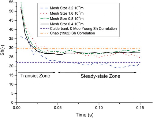
According to the Batchelor length scale, the required minimum mesh size is 0.67·10⁻⁴ m for having the realistic concentration gradients in our case. The independent mesh size on mass transfer was found in the range of the Batchelor length scale. The influence of the mesh size on diminishing bubble diameters (calculated with an assumption of spherical bubble) is shown in Figure 12. The influence of the mesh size on the bubble diameter disappears after the second mesh refinement. Figure 13 shows the influence of the grid resolution on the numerical Sherwood number against time. Oscillations are observed at a lower grid resolution, perhaps due to the parasitic currents and/or huge concentration difference at the interface cells. They disappear only with the finest mesh size. After the second mesh refinement, the Sherwood number approaches 27 (see Table 3).

Figure 12. Influence of mesh size on the normalized diameter of the bubble versus time using the PLIC-1 method in 2D. Note: P.O. = pressure outlet.

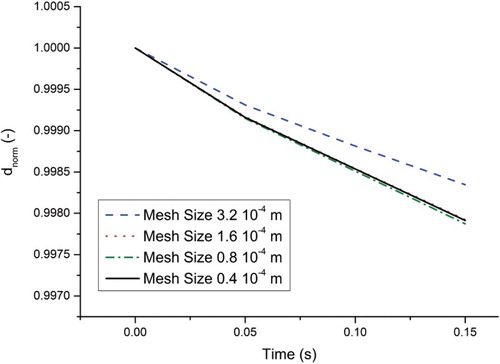
Figure 13. Influence of grid resolution on the numerical Sherwood number using the PLIC method.

4. Conclusions

In this present direct numerical mass transfer investigation for a free-rising bubble, two numerical methods (PLIC-1 and PLIC-2) of calculating discrete interfacial concentration gradients at the interface cells were compared, and the results are very similar. The PLIC-1 method is more accurate but also more time consuming than the PLIC-2 method. The interfacial mass transfer source term in the mass balance equation was linked to the void fraction and the species conservation equation using a DMT macro in ANSYS FLUENT.

The results of the numerical Sherwood number are in accordance with the theoretical results as long as sufficient grid resolution and high-order schemes for spatial discretization with low time-step sizes are implemented. However, the challenge of direct measurement of the local concentration field in two-phase flows makes it difficult to quantitatively evaluate the comparison of numerical results with experimental results. This developed tool works well for immiscible fluids when their density ratio is around unity. Deviation from unity causes mismatching of the mass flow rate and the volume shrinkage rate. In order to provide the balance of mass and volume change, the void fraction equation as well as the velocity field at the interface should be defined accordingly. Therefore it is more meaningful to use the individual source term macros instead of the DMT macro.

Disclosure statement

No potential conflict of interest was reported by the authors.

References

- ANSYS. (2009). FLUENT theory guide, user guide.
- Batchelor, G. K. (1959). Small-scale variation of convected quantities like temperature in turbulent fluid Part 1. General discussion and the case of small conductivity. Journal of Fluid Mechanics, 5, 113–133. doi: 10.1017/S002211205900009X
- Bothe, D., Koebe, M., Wielage, K., & Warnecke, H. J. (2003). VOF-Simulation of mass transfer from single bubbles and bubble chains rising in aqueous solutions. In Proceedings of the Fourth ASME—JSME Joint Fluids Engineering Conference. Hawaii, USA.
- Calderbank, H., & Moo-Young, M. B. (1961). The continuous phase heat and mass-transfer properties of dispersions. Chemical Engineering and Science, 16, 39–54. doi: 10.1016/0009-2509(61)87005-X
- Chao, B. T. (1962). Motion of spherical gas bubbles in a viscous liquid at large Reynolds numbers. Physics of Fluids, 5, 69–79. doi: 10.1063/1.1706493
- Francois, J., Dietrich, N., Guiraud, P., & Cock, A. (2011). Direct measurement of mass transfer around a single bubble by micro-PLIFI. Chemical Engineering Science, 66, 3328–3338. doi: 10.1016/j.ces.2011.01.049
- Kreutzer, M. T., Kapteijn, F., Moulijna, J. A., & Heiszwolf, J. J. (2005). Multiphase monolith reactors: chemical reaction engineering of segmented flow in microchannels. Chemical Engineering Science, 60, 5895–5916. doi: 10.1016/j.ces.2005.03.022
- Kröger, M., Alke, A., Bothe, D., & Warnecke, H. J. (2007). A VOF-based approach for the simulation of reactive mass transfer from rising bubbles. In Proceedings of 4th International Berlin Workshop on Transport Phenomena with Moving Boundaries (pp. 290–301). Berlin, Germany.
- Oezkan, F. (2013). Investigation and modeling of heterogeneously catalyzed G/L reactions in microreactors. Karlsruhe: PhD Thesis, Karlsruhe Institute of Technology.
- Onea, A. (2006). Numerical simulation of mass transfer with and without first order chemical reaction in two-fluid flows. PhD Thesis, University of Karlsruhe, Department of Mechanical Engineering.
- Özkan, F., Wörner, M., Wenka, A., & Soyhan, H. S. (2007). Critical evaluation of CFD codes for interfacial simulation of bubble-train flow in a narrow channel. International Journal for Numerical Methods in Fluids, 55, 537–564. doi: 10.1002/fld.1468
- Ozmen-Cagatay, H., & Kocaman, S. (2011). Dam-break flow in the presence of obstacle: Experiment and CFD simulation. Engineering Applications of Computational Fluid Mechanics, 5(4), 541–552. doi: 10.1080/19942060.2011.11015393
- Qian, D., & Lawal, A. (2006). Numerical study on gas and liquid slugs for Taylor flow in a T-junction microchannel. Chemical Engineering Science, 61, 7609–7625. doi: 10.1016/j.ces.2006.08.073
- Raymond, F., & Rosant, J. M. (2000). A numerical and experimental study of the terminal velocity and shape of bubbles in viscous liquids. Chemical Engineering Science, 55, 943–955. doi: 10.1016/S0009-2509(99)00385-1
- Sato, T., Jung, R. T., & Abe, S. (2000). Direct simulation of droplet flow with mass transfer at interface. ASME Journal of Fluids Engineering, 122, 510–516. doi: 10.1115/1.1287504
- Wang, S., Su, Y., Wang, Z., Zhu, X., & Liu, H. (2014). Numerical and experimental analyses of transverse static stability loss of planing craft sailing at high forward speed. Engineering Applications of Computational Fluid Mechanics, 8(3), 44–54. doi: 10.1080/19942060.2014.11015496
- Wielage, K. (2005). Analysis of non-newtonian and two phase flows. Paderborn: Dissertation, University of Paderborn.
- Youngs, D. L. (1982). Numerical methods for fluid dynamics. New York: Academic Press.