Insights derived from CFD studies on the evolution of planar wall jets

ABSTRACT

The main objective of this paper is to demonstrate that a simple and cost-effective 2D Reynolds-averaged Navier–Stokes (RANS) simulation approach can often be efficiently used in industrial design applications. We simplified the designing approach of a racetrack jet dryer to a problem involving the streamwise evolution of an offset wall jet. We compared our simple 2D RANS simulations with experiments and large eddy simulation (LES), and were encouraged to see that our simplified approach produced a better correlation with the experiments compared to LES, which is expected to be much more accurate (even though computationally orders of magnitude more expensive). We conclude that under certain circumstances a simple 2D approach can lead to a dependable solution. Additionally, we used the results from these simulations to enhance our understanding of the evolution of offset wall jets. The insights derived from these simulations suggest the existence of scaling parameters that can express offset wall jets as a family of self-similar flows.

KEYWORDS:

• CFD
• RANS
• wall jet
• offset wall jet
• jet dryer

1. Introduction

The National Association for Stock Car Auto Racing (NASCAR) is the largest sanctioning body for auto racing in the United States (US), and the NASCAR Sprint Cup Series is the premier motorsports competition in the US. From the point of view of television-viewer popularity, it is second only to the National Football League (NFL) Super Bowl. NASCAR racecars race on slick tires meant for dry racetracks. As such, whenever it rains the race needs to be stopped or red-flagged until the track has dried out completely. From a private communication with NASCAR's Managing Director of Business Planning and Operations, Mr. Shawn Rogers, we understood that for every minute of rain-induced delay, the TV viewer-ship drops significantly, which has an adverse commercial impact. Subsequently, NASCAR feels that it is critical for them to reduce this downtime by improving the existing racetrack drying methodology, which includes both the redesign of existing drying equipment and on-track dryer movement pattern.

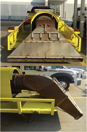
A typical NASCAR track jet dryer consists of a nozzle mounted at the exhaust end of an aircraft-type jet engine. The hot exhaust out of the jet engine is used to dry the wet tracks. As can be seen in Figure 1, these jet dryers show a wide range of variations both in terms of the jet engine and the shape of the exhaust nozzle that is mounted at the engine exhaust end. In the most common variant of these jet dryers, used during 2012 race season, the hot jet engine exhaust is discharged on the track from a rectangular exit. If one ignores the effect of the side walls, this discharge can be simplified as a planar jet. Since this jet impinges on the racetrack, from a pure fluid dynamics point of view, it can be treated as an offset wall jet. The jet has two effects on the layer of rainwater on the track: firstly, it scrapes the fluid film and atomizes it, and secondly, the heat in the exhaust causes evaporation. Since turbulence enhances mixing and evaporation, it was conjectured that a well-controlled turbulent jet with a low spreading rate and a nearly uniform turbulent kinetic energy (TKE) distribution in the wall-normal direction would have a better drying-time efficiency. The low spread rate of the jet will maximize the time period during which the water film is in contact with the hot jet exhaust. This means that an optimum design of such a device boils down to the problem of controlling the jet spread and its turbulent characteristics which, in turn, requires a good understanding of the spatial evolution of an offset wall jet.

Figure 1. The two most widely used variants of NASCAR racetrack jet dryers.

A wall jet, as shown in Figure 2, is obtained when a fluid stream is injected along a wall at a velocity higher than the ambient flow. Figure 2 also shows the coordinates system used in this study, along with the parameters pertinent to the study of wall jets. Per this figure, and are the streamwise and wall-normal coordinates while and are the velocity components in and , is the jet width, is the jet bulk velocity at the exit, is the maximum value of the velocity at a given , and is the wall-normal location of at that location. All symbols used in this study are defined in the nomenclature section at the end of the paper.

Figure 2. The schematic configuration of a planar wall jet.

Evidently, the study of wall jets presents one level of complexity over basic flows as this involves an interaction of two canonical flows: one edge of this flow is a free shear flow while the other one is wall bounded. Besides being a topic of popular fundamental interest, wall jets have been widely investigated because of their importance in various practical engineering and environmental applications. Examples include, but are not limited to, the exhaust of vehicles (Ockfen & Matveev, 2009), the cooling of energy-conversion devices (e.g., film cooling of gas turbine blades; Ashok Kumar & Prasad, 2009) and, environmental problems, (e.g., horizontal outfall near the seabed modeled as the submerged discharge of a dense jet; Shao & Law, 2011).

From a fundamental point of view, the most distinctive and interesting feature of a wall jet is the interaction between the near-wall layers. The inner layer of the planar wall jet is similar to that of the turbulent boundary layer, while the outer layer resembles that of a free (planar) jet. The interaction of large turbulence scales in the outer layer with smaller scales in the inner layer creates a complicated flow field and determines the development of the wall jet.

The development and characterization of wall jets has been studied extensively in the past using both experimental and numerical investigations – cf. Bourque and Newman (1960), Bourque (1967), Launder and Rodi (1981), Hoch and Jiji (1981), Nasr and Lai (1998), Eriksson, Karisson, and Persson (1998), and Gao and Ewing (2007) to name but a few. These works, which span a period of more than forty years, involved both wall jets tangential to the wall and wall jets with a small offset distance from the wall, the so-called ‘offset wall jet’. For instance, Eriksson et al. carried out laser Doppler velocimetry (LDV) measurements in a planar turbulent wall jet attached to the wall at a Reynolds number of 9600 in which the inner region of the flow () was specifically investigated. Nasr and Lai studied both experimentally and numerically the mean velocities and turbulent characteristics of a jet with an offset ratio, defined as , of 2.125. Here, is the jet width, and is the vertical offset of the jet from the wall. In their LDV measurements, Nasr and Lai observed a high turbulence recirculating flow near the nozzle exit between the jet and the offset wall. In the computational fluid dynamics (CFD) part of their project, they tested the veracity of three different turbulence models to predict this type of flow and concluded that the standard turbulence model produced the best agreement between CFD and their LDV measurements. More recent experimental investigations of turbulent planar wall jets include those by Gao and Ewing, and Rostamy, Bergstrom, Sumner, and Bugg (2011). Gao and Ewing studied the development of the planar jets at a Reynolds number of 44,000. They observed that the normalized jet reattachment distance was approximately 6 for , a value that decreases with the increase of offset distance. A more recent study by Rostamy et al. would have been more relevant to the ultimate objective of this project had it been carried out at a higher Reynolds number with wall offsets; their study included the effects of surface roughness on the jet development. This study was carried out at a Reynolds number of 7500 and considered the development of wall jets on both smooth and transitionally rough walls; they used 36-grit sandpaper to create a rough wall. They quantified the effect of roughness on the momentum field and found that it caused up to a 140% increase in skin friction coefficient when compared to the smooth wall. They concluded that this effect is mostly confined to the inner region of the wall jet, where it causes increased thickness of the inner layer and a faster streamwise decay rate of the maximum velocity. However, the spread rate of the jet seems to be unaffected by the roughness and, thus, roughness has minimal effect on the characteristics of mean flow in the outer region of the flow.

Researchers have used many forms of numerical simulation techniques, including direct numerical simulation (DNS; Ahlman, Brethouwer, & Johansson, 2007), large eddy simulation (LES; Dejoan, & Leschziner, 2005; Le Ribault, Sarkar, & Stanley, 1999; Uddin, Pollard, & Braly, 2004) and Reynolds-averaged Navier–Stokes (RANS; Craft, Graham, & Launder, 1993; Raisee, Noursadeghi, Hejazi, Khodaparast, & Besharati, 2007; Tangemann, & Gretler, 2000). The two-equation eddy-viscosity-based turbulence models used by Craft et al. (1993) appeared to over-predict the TKE production by almost an order of magnitude which leads to high entrainment of the free stream fluid and, thus, the wall jet becomes too thick while the level of peak velocity becomes too low. However, the more recent simulations of Tangemann and Gretler (2000) using a standard model show significant improvement: their results showed very good agreement with the experimental measurements.

As a part of the optimum jet dryer nozzle design, it became essential to investigate the effects of the nozzle aspect-ratio and offset distance on the flow evolution. Since this process requires a large number of simulations to be run with a number of nozzle shapes and offset distances, it was decided that a RANS-based CFD approach would be the best option. In order to make the design process even faster, 2D simulations were used as the first-order design decision arbitrator. The data sets presented in this paper were generated from this point of view. Because of the uncertainties associated with RANS predictions, a sanity check for the CFD procedure is required which, among other things, require the identification of the most optimum turbulence model and mesh setup. The experimental data of Eriksson et al. (1998) and Gao, & Ewing (2007) were used for this purpose.

2. Computational details

2.1. Governing equations

Using Einstein's compact notation, where the repeating index variable represents the sum over all possible values, the time-averaged or RANS equations can be written as follows:

Continuity Equation: (1)

Momentum Equation: (2) where the overbar denotes a temporal or time-averaged quantity, represents the effect of external body forces, and is the rate of strain defined as (3)

In a based RANS model, two additional transport equations are solved: one for , the TKE, and the other for the rate of kinetic energy dissipation or simply dissipation . The transport equations for and are:

TKE: (4)

Dissipation: (5) where is the kinematic eddy viscosity, and , , , , and are closure coefficients. In the standard model, the kinematic eddy viscosity is defined as and the closure coefficients are set as , , , , and . In the realizable model, is expressed as a function of the mean flow and turbulence properties, rather than assumed to be constant as in the standard model: (6)

Here, the constants and are given by and , where , and .

The model is another two-equation model family which, like the family, solves a transport equation for but, instead of it solves a transport equation for , the specific dissipation rate or dissipation rate per unit TKE. However, the family of turbulence modeling uses a different transport equation for and a somewhat modified definition for the eddy viscosity, where , and .

TKE: (7)

Specific dissipation rate: (8)

Closure coefficients and auxiliary relationships for the standard turbulence model are: and the vorticity tensor .

Compared to the standard, the Shear Stress Transport (SST) model adds an additional non-conservative cross- diffusion term in the TKE equation containing the dot product .

2.2. Computational grids and STAR-CCM+ discretization

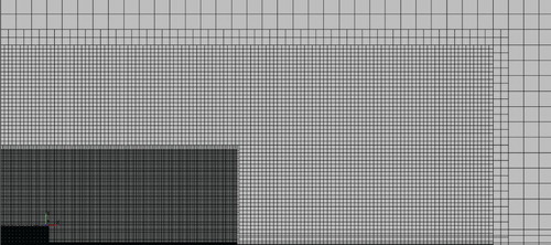
All simulations presented in this paper were carried out on a 16-core 256 GB RAM HP Z820 workstation using the commercial CFD code STAR-CCM+ (version 7.04) by CD-ADAPCO. During the pre-processing stage, another commercial package (ANSA) was used for geometry preparation and surface meshing. STAR-CCM+ was used for volume meshing, simulation and post-processing operations. All simulations were performed at the Reynolds number, based on the bulk inlet velocity and jet height, of 9600 to match the experiments of Eriksson et al. (1998). A 7×1.45 m tank with a nominal jet height of 9.6 mm was used; the computational domain had the same size and consisted of 47,500 cells in 2D. As can be seen from Figure 3, very fine mesh was used in the region around the jet; the streamwise and wall-normal extents of this fine mesh region are and respectively. An even finer mesh was applied to the very beginning of the jet exit, with streamwise and lateral extents of and respectively.

Figure 3. The computational domain and mesh.

STAR-CCM+ is a finite-volume-based code where a second-order discretization is used for the source and diffusion terms while the second-order upwind scheme is used for the convection terms in the case of steady-state simulations. The segregated flow model in STAR-CCM+ used in this study solves the flow equations in a segregated, or uncoupled, manner. The linkage between the momentum and continuity equations is achieved with a predictor-corrector approach. The complete formulation can be described as using a collocated variable arrangement (as opposed to staggered) and a Rhie, and Chow (1984) pressure-velocity coupling combined with a SIMPLE-type algorithm.

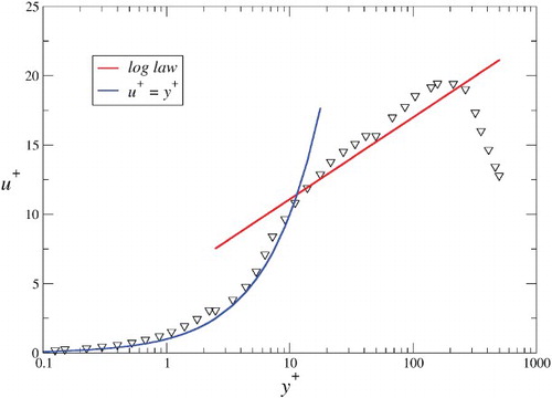
In order to verify whether the mesh resolution used in this study is sufficient or not, in Figure 4, a mean velocity distribution is presented in inner flow scaling at . In this figure the blue line represents and the red line represents the log-law of the wall , where the characteristic constant the von Karman constant , , the wall shear velocity and is the wall shear stress. Figure 4 shows that the flow is very resolved at the wall with a large number of data points in the region .

Figure 4. Mean velocity distribution in inner scaling at .

3. Results

3.1. Turbulence model veracity check

RANS CFD predictions of the wall shear velocity () and , the location (the local maximum mean streamwise velocity), at are compared with those from the experiment and LES simulations in Table 1. The RANS models considered include:

• the standard model of Launder, & Spalding (1974) with the two-layer wall treatment of Rodi (1991),

• Realizable model of Shih et al. (1995) with two-layer wall treatment,

• Standard model of Wilcox (2006) with all wall treatment

• the SST model of Menter (1994) with all wall treatment. The term wall treatment, requires some additional clarification.

Table 1. Comparison between the experimental and CFD-predicted values of the normalized wall friction velocity and location of the maximum streamwise mean velocity at .

Case
Experiment (Eriksson et al., 1998)	0.05244	167
LES (Dejoan & Leschziner, 2005)	0.04692	138
RANS Standard with two-layer wall treatment	0.05350	159
RANS Realizable two-layer wall treatment	0.05332	158
RANS Standard all y+ wall treatment	0.05318	158
RANS SST all y+ wall treatment	0.04948	122

Wall treatment in STAR-CCM⁺ is a set of near-wall modeling assumptions for each turbulence model. This term is a little different from the traditional wall functions, which refers to only one type of wall treatment. Three types of wall treatment are available in STAR-CCM⁺, per the user manual:

• The high wall treatment implies the traditional wall-function-type approach which assumes that the near-wall cell lies within the logarithmic region of the boundary layer or the wall node ;

• The low wall treatment assumes that the near wall mesh is resolved to viscous sublayer , and thus no wall function is applied;

• The all wall treatment is a hybrid treatment that attempts to emulate the high-wall treatment for coarse meshes, and the low-wall treatment for fine meshes. It is also formulated with the desirable characteristic of producing reasonable answers for meshes of intermediate resolution (that is, when the wall-cell centroid falls within the buffer region of the boundary layer).

It is rather fortuitous in Table 1 that our RANS predictions of both and appear to match better with the experiment than those from the carefully executed well-resolved LES studies of Dejoan and Leschziner (2005). In their work the wall-nearest computational domain is located at in the wall region, while in the outer shear layer ranges from 0.02 to 0.05; the streamwise and lateral direction, and are kept approximately at 24 and 23 respectively. The RANS predictions of is within 2% of the experiment, while the LES predictions are off by 10%. Similarly, except for the SST model, RANS predicted the location of maximum mean velocity within about 5%, while the LES predictions are off by as much as 17%. Overall, the agreement between our 2D CFD predictions and the experiment is excellent; however, it appears that the standard turbulence model is slightly better than the rest; thus, it was subsequently used to predict the jet flow development with other wall offsets. It can be noted that Nasr and Lai (1998) also came to a similar conclusion. Although not shown on the table, the standard model with all wall treatment shows results which are off by about 50%, and hence is excluded from all discussions. This simply implies that the traditional wall function approach should be avoided in RANS-based CFD analysis of wall jet flows.

The two approaches of wall treatments used in this study, viz. the two-layer and all , require some further corroboration. The two-layer approach allows the model to be applied in the viscous sublayer where the computation is divided into two layers. The first layer is the layer next to the wall where the turbulent dissipation rate and the turbulent eddy viscosity are specified as functions of the wall distance. The values of specified in the near-wall are then blended smoothly with the values computed from solving the transport equations far from the wall. However, the equation for the TKE is solved in the entire flow. The all wall treatment is a hybrid treatment that emulates a wall treatment depending on the value of the wall node: (a) the high wall treatment, which implies the wall function approach, if the mesh is too coarse and (b) a low wall treatment for the finer mesh if the wall node lies in the viscous sublayer, that is .

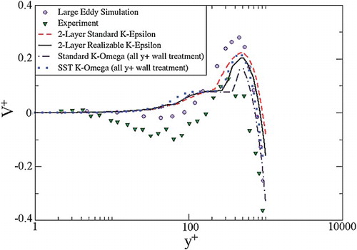
Streamwise and wall-normal velocity distributions at obtained from our CFD simulations are compared against the experiment and LES predictions in Figures 5 and 6. Except for the SST model, the rest appear to show very good correlations with the experiment. It is a pleasant surprise that our RANS predictions, like the predictions of the wall shear velocity and the location of the maximum streamwise mean velocity, are closer to the experiments than the LES predictions. The wall-normal velocity predictions, however, do not show the same degree of correlation. Although the CFD predictions in the inner and outer regions match fairly well with the experiment, they differ significantly in the region . However, the LES and RANS approach shows a reasonably good match in this regime. As mentioned earlier, compared to the LES of Dejoan and Leschziner (2005), our RANS predictions of are a better match with experiment. This, in turn, results in a better match between the RANS CFD and the experimental values of the streamwise and wall-normal mean velocities in inner flow scaling. Dejoan and Leschziner explain this discrepancy between the LES and experiment in terms of the inability of the LES approach to capture the transition in the outer shear layer and in the boundary layer with very high accuracy, as the prediction of transition shows sensitivity to resolution, the perturbations present at the discharge plane and the sub-grid-scale model. The reason of the mismatch between the RANS prediction and the experiment probably lies with the wall function approach, which heavily relies on the existence of the log-law of the wall which is particularly valid for the streamwise component of the flow only. This discrepancy indicates that additional refinement to the wall treatment is required to make this approach better predict non-tangential velocity components.

Figure 5. Profiles of the streamwise velocity at , scaled with inner variables.

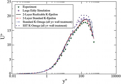
Figure 6. Profiles of the wall-normal velocity at , scaled with inner variables.

Profiles of Reynolds shear stress at equal to 10 and 20 are shown in Figure 7. When compared to the Eriksson et al. (1998) data, the predicted profiles show good agreement with the experiment except for the region at . This slight lack of agreement can, partly, be linked to the under-prediction of the wall-normal velocity component, as in Figure 6. However, the discrepancy in the prediction of Reynolds stress is less prominent than that of the wall-normal velocity in inner-flow scaling. Additionally, the peak values of the shear stress at both and 20 are slightly over-predicted.

Figure 7. Comparison between the experimental data and CFD predictions of Reynolds shear stress at and 20.

The jet half-width at a given streamwise location is defined as the cross-stream distance at which the velocity is equal to . It is often the most quoted cross-stream length scale in an evolving jet, and its round simple jet counterpart is the jet half-radius . The CFD-predicted (using the realizable turbulence model) streamwise evolution of the jet half-width is compared with the experiments of Eriksson et al. (1998) in Figure 8.

Figure 8. Comparison between the experimental and CFD-predicted (a) jet growth rate and (b) decay of streamwise mean velocity.

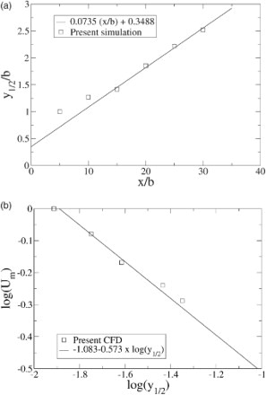
By fitting their experimental data, Eriksson et al. showed that there exists a linear relationship between and . They expressed the relationship as which is shown in Figure 8(a) as a solid line. Figure 8(b) shows that the RANS-predicted results are in excellent agreement with the experimental results. The exponential decay of the jet maximum velocity can also be investigated by plotting the maximum jet velocity against the jet half-width on a log-log plot, as in Figure 8(b). This, again, shows a good correlation between the experiment and our CFD.

3.2. Effect of jet offset

To facilitate the discussion on the effect of jet offset, the distinctive flow regimes in a wall jet are shown schematically in Figure 9 using the conventions of Nasr and Lai (1998). In this figure, a Cartesian coordinate system is used with the origin of the coordinate system at the intersection of the nozzle plate and the wall. The x-axis is measured in the flow direction along the wall and is the cross-stream wall-normal direction. A planar incompressible, turbulent air jet is discharged parallel to the wall from a plane nozzle with an offset distance above the wall and represents the jet width. As shown in the figure, there are three discernible regions in an evolving offset wall jet: (i) the converging region, (ii) the reattachment region, and (iii) the wall jet region. The converging region is the low pressure zone formed in the area bounded by the jet and the wall. This causes the jet to develop towards the wall and eventually attach to the wall at the reattachment point or impingement point. The lower part of the jet is deflected upstream from the reattachment point into the low pressure region, forming a recirculation zone. In the reattachment region, the jet flow is strongly affected by the boundary layer developing on the wall. However, downstream of the reattachment region, in the wall jet region, the flow continues to develop as a normal no-offset wall jet.

Figure 9. Schematic diagram of an offset jet showing zones of primary interest.

The locus of , where represents the value corresponding to the maximum of the local mean streamwise velocity at a given , is shown in Figure 9. It can be seen that in the converging and reattachment regions has a downward trend implying that decreases as the flow evolves downstream. However, the onset of the wall jet region is marked by the reversal of this trend when reaches its minimum and starts to increase slowly with increasing . Essentially, this converging region is the major difference between an offset wall jet and a simple wall jet. In some ways, the offset wall jet flow and the flow past a backward-facing step have few topological characteristics in common. It is seen in the literature that, for a backward-facing step flow, two-equation turbulence models have trouble predicting the flow separation and recirculation as well as Reynolds stresses. The numerical investigations of Thangam and Spezialet (1992) suggested that for the turbulent flow past a backward-facing step, when compared to other turbulence models, the standard model can yield good predictions with eddy viscosity modifications. The offset wall jet has similar flow development except that it has an additional outer shear layer. Based on this and our earlier conclusion with no offset wall jet, we investigated the effect of the wall offset using the two-layer standard model. A total of four offset distances of equal to 0.5, 1.0, 1.5 and 2.0 are considered.

In order to investigate the effect of wall offset on the downstream evolution of wall jets, plots of the streamwise variations of and are shown in Figures 10 and 11 respectively using two different forms of scaling: is scaled by the reattachment length () in top profiles and by the jet height () in bottom profiles. Both of these two figures show good resemblances with Gao and Ewing's (2007) experiment. Figure 10 (top) suggests that the decay rate prior to the reattachment is non-linear, and the order of non-linearity depends strongly on . However, up to , these profiles seem to show a regional self-similarity, i.e., all of the profiles collapse to each other with essentially constant at 1. This region is very similar to the laminar core region of a free jet. This decay stops at certain values, which seems strongly influenced by . Beyond this point, the streamwise development of goes through a transition before the decay of becomes linear, like a free jet. Though, at this point in time, it is unclear what factors determine the onset of this linear decay region, the almost constant rate of linear decay of for all of the profiles suggests the existence of possible scaling parameters. Due to the limited number of profiles considered in this study, combined with the uncertainties of the RANS simulations, further conclusions regarding this matter are not drawn.

Figure 10. The streamwise decay of the maximum streamwise local mean velocity ; is scaled with the reattachment length (top), and with the jet height (bottom).

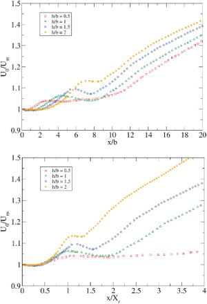
Figure 11. The streamwise evolution of the jet half-width (); is scaled with the reattachment length (top), and with the jet height (bottom).

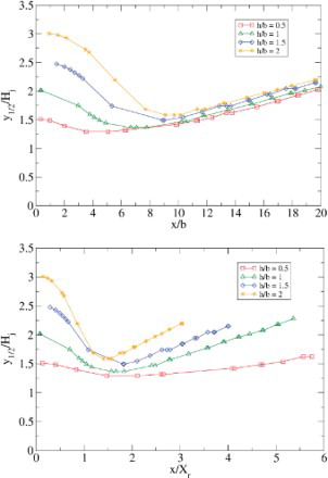
It appears from Figure 11 that for all of the ratios considered in this study, for smaller, the jet half-width drops with non-linearly until it reaches its minimum, and then starts to increase linearly. Like the profiles, the non-linear rate at which drops off is a strong function of , while the growth rate of in the linear region seems to be constant and independent of . Note that in these plots is scaled with the jet height . However, the plots in Figure 10 (bottom) suggest that, if an alternative scaling which is again a function of is used instead, profiles corresponding to various are likely to collapse onto a single curve. However, because of the limitations cited earlier, further analysis is not provided, and the need for additional work is emphasized.

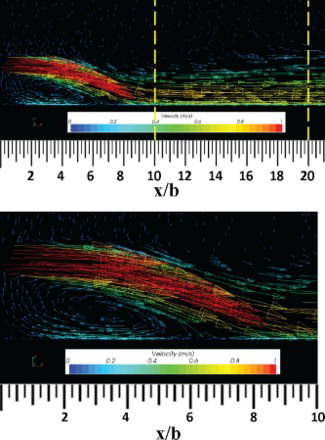
The flow regions of an evolving offset wall jet become distinctive as the wall offset increases. For that matter, the mean velocity vectors corresponding to the offset distance are shown in Figure 12. The zoomed-in view shows the entire recirculation region and the beginning of the reattachment region. Downstream of the recirculation region, the flow starts to develop as a traditional wall jet. For this , the reattachment length appears to be approximately equal to which compares very well with the experimental value of from Nasr and Lai (1998). Although, this slight discrepancy is not discernible, the under-prediction of the reattachment length is not unexpected, as studies involving backward-facing steps also show that the two-equation standard model tends to under-predict reattachment lengths (cf. Lakehal & Rodi, 1997). The detached vortical flow in the recirculation region is characterized by a low-pressure vortex core and strong reverse or back-flow. In addition to the reattachment length, the other two often-quoted characteristics of this type of separation bubble are the magnitude and location of the maximum back-flow velocity. The CFD-predicted maximum back-flow velocity of and its streamwise location of compare very well with the experimental values of and respectively, again from Nasr and Lai (1998). These indicate that our CFD has captured the dynamics in the recirculation region very well.

Figure 12. Mean velocity vectors corresponding with the wall offset of , whole flow view (top), and zoomed-in view (bottom).

Contour plots of mean streamwise velocity are shown in Figure 13 for all five jet offsets considered in this study. At , the maximum velocity extends to , and at it only reaches out to . This indicates that the larger the offset distance, the lower the streamwise velocity at the reattachment point. The vertical velocity distributions in Figure 14 show that the jet is moving more towards the wall. In other words, an increasing wall distance will cause a stronger vertical velocity when the jet gets reattached. At the same time, a higher positive vertical velocity close to the jet exit in the converging region indicates stronger recirculation behavior. In terms of jet dryer nozzle design (which was the original intent of this project), the nozzle cannot be too far away from the wall since the larger the offset distance, the shorter the high streamwise velocity. This means that the jet will not cover as much longitudinal area over the racetrack.

Figure 13. Contours of the mean streamwise velocity with , 0.5, 1.0, 1.5 and 2.0.

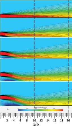
Figure 14. Contours of the mean wall-normal velocity with , 0.5, 1.0, 1.5 and 2.0.

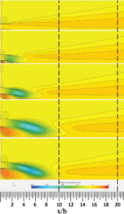
However, the flow that comes out of the nozzle has to have both a sufficiently strong streamwise velocity and a downward velocity to be able to scrape the water off the track, which will make the evaporation process more efficient. So, the negative vertical velocity component of the jet also has a positive impact on the efficiency of the jet dryer. Besides, the recirculation zone caused by the offset can be treated as a minor jet to dry the area behind the main jet flow.

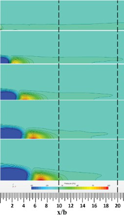
Looking at the pressure distribution for different offset jets in Figure 15, a low-pressure region is formed close to the nozzle exit. This is because the jet converges toward the wall as it proceeds downstream from the nozzle, forming the recirculation zone as mentioned earlier. The positive pressure area after it is the reattachment region, where the peak value occurs at the reattachment point. A larger positive pressure area means more interaction between the jet and the wall. In other words, the moisture exchange in that area is faster, and as a result, the drying efficiency is better in the region.

Figure 15. Contours of the mean pressure with , 0.5, 1.0, 1.5 and 2.0.

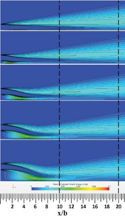
The TKE produced by shear stresses is characterized by the RMS velocity fluctuations. In RANS, it is quantified by the mean of turbulence normal stresses . Figure 16 shows the contours of TKE for all offset distances. We can see that the flow is highly turbulent at the reattachment location and at the offset distance of , while the TKE is relatively low on the ground with smaller offset distances or even no offset. It was conjectured that a higher TKE and turbulence intensity would improve the drying efficiency in certain areas.

Figure 16. Contours of the mean TKE with, 0.5, 1.0, 1.5 and 2.0.

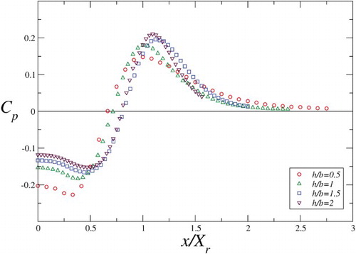
The streamwise mean wall pressure coefficient variations for different offset distances are shown in Figure 17. The static wall pressure for all offset distances decreases to the minimum at approximately , which is a little different from the value of 0.65 reported by Gao and Ewing (2007). One of the reasons that might have caused this discrepancy is the higher Reynolds number (Re = 44,000) used in Gao and Ewing which may have caused a longer reattachment length. Figure 16 also shows that the pressure increases rapidly to the maximum value in the reattachment region. The magnitude of the maximum and minimum values of the pressure coefficients increase when the offset distance of the jet increases; this is due to the differences in the trajectory of the jet toward the wall. The mean wall pressure downstream of the reattachment point decreases to the free-stream pressure more gradually in jets with lower offset distances, indicating that these jets recovered more smoothly (Gao & Ewing, 2007).

Figure 17. Streamwise distributions of the wall pressure coefficient for different jet offsets.

Figure 18 shows the reattachment length for the jets with in the range 0.5 to 2. This figure also contains the experimental results of Lund (1986). The CFD-predicted results agree well with the experimental data except for one data point at, which might just be an outlier among the cases that have been studied. The reattachment point of the jet is moving forward along the streamwise direction with increasing offset distances. A similar conclusion can be seen in the work of Gao and Ewing (2007).

Figure 18. Dependence of the reattachment length on the wall offset.

4. Conclusion

In summary, RANS simulations of planar turbulent wall jets with small offset distances have been performed with an objective of investigating the efficacy of 2D simulations in industrial design applications. The first part of this study involves the establishment of a best practice for simulating a flow that resembles our application; this step involves setting up correct discretization strategies and choice of turbulence models. This was accomplished by comparing our 2D CFD results with those obtained from experiments and LES. The parameters of our interest include crucial factors that impact the effectiveness of a typical jet dryer; these include the jet reattachment length, the location of the maximum streamwise velocity, wall friction, and the streamwise velocity, pressure, and TKE distributions. The specific conclusion drawn from this study are:

• In general, 2D RANS simulations have good agreements with the experimental results of Eriksson et al. (1998). In this particular case, results from the realizable , standard , SST and standard models fared well in terms of predicting the mean velocity of the jet along the streamwise direction. However, the standard model with two-layer approach is slightly favorable.

• From a better agreement between our 2D RANS predictions of the wall shear velocity, the location of the maximum streamwise mean velocity, and velocity distributions with the experimental results, we conclude that, under some circumstances, a 2D RANS approach can outperform LES predictions of the same quantities.

• Our simulations indicate that additional refinement to the wall-function approach of turbulence modeling is required in order to achieve a reliable prediction of the wall-normal component of turbulent fluctuations.

• With a small offset distance, the jet has a greater streamwise velocity near the nozzle exit and less recirculation effect. In terms of the jet dryer designing process, a small offset jet will help to scrape water off the track more efficiently.

• With a relatively large offset distance, jets will have a higher vertical velocity in the reattachment region and a higher TKE, which will lead to more effective evaporation. Thus, an optimum design requires something in between these two.

In conclusion, 2D wall jet studies could be the first step in designing or improving a racetrack jet dryer. Further work involving 3D simulations with heat transfer are necessary to investigate how the nozzle aspect ratio, side wall boundary layers, flow temperature and other factors will impact the drying efficiency and, thus, the design.

5. Nomenclature

	=	Jet height
	=	Pressure coefficient
	=	Offset distance of the wall from the edge of the nozzle
	=	Reynolds number
	=	Mean streamwise velocity
	=	Mean streamwise velocity at the nozzle exit
	=	Local maximum streamwise velocity
	=	Dimensionless streamwise velocity,
	=	Friction velocity
	=	Reynolds shear stress
	=	Mean lateral velocity
	=	Dimensionless lateral velocity,
	=	Spatial coordinate in the streamwise direction
	=	Reattachment length (offset wall jet)
	=	Spatial coordinate in the wall-normal direction
	=	Jet half-width, the y position at which
	=	Wall-normal location of
K	=	Von Karman constant
ν	=	Kinematic viscosity

Disclosure statement

No potential conflict of interest was reported by the authors.

Funding

This work was supported by a NASCAR grant against UNCC proposal number 2012-0777.

References

- Ahlman, D., Brethouwer, G., & Johansson, A. V. (2007). Direct numerical simulation of a plane turbulent wall-jet including scalar mixing. Physics of Fluids, 19, 065102. doi: 10.1063/1.2732460
- Ashok Kumar, M., & Prasad, B. V. S. S. S. (2009). Computational investigation of flow and heat transfer on an effused concave surface with a single row of impinging jets for different exit configurations. Engineering Applications of Computational Fluid Mechanics, 3(4), 530–542. doi: 10.1080/19942060.2009.11015289
- Bourque, C. (1967). Reattachment of a two-dimensional jet to an adjacent flat plate. Advances in fluidics (pp. 192–204). New York: ASME.
- Bourque, C., & Newman, B. (1960). Reattachment of a two-dimensional jet to an adjacent flat plate. Aeronaut Quart, 11, 201–232.
- Craft, T. J., Graham, L. J. W. & Launder, B. E. (1993). Impinging jet studies for turbulence model assessment—II. An examination of the performance of four turbulence models. International Journal of Heat and Mass Transfer, 36(10), 2685–2697. doi: 10.1016/S0017-9310(05)80205-4
- Dejoan, A., & Leschziner, M. A. (2005). Large eddy simulation of a plane turbulent wall jet. Physics of Fluids, 17(2), 025102. doi: 10.1063/1.1833413
- Eriksson, J. G., Karisson, R. I., & Persson, J. (1998). An experimental study of a two-dimensional plane turbulent wall jet. Experiments in Fluids, 25(1), 50–60. doi: 10.1007/s003480050207
- Gao, N., & Ewing, D. (2007). Experimental investigation of planar offset attaching jets with small offset distances. Experiments in Fluids, 42(6), 941–954. doi: 10.1007/s00348-007-0305-3
- Hoch, J., & Jiji, L. M. (1981). Two-dimensional turbulent offset jet-boundary interaction. Journal of Fluids Engineering, 103, 154–161. doi: 10.1115/1.3240766
- Lakehal, D., & Rodi, W. (1997). Calculation of the flow past a surface-mounted cube with two-layer turbulence models. Journal of Wind Engineering and Industrial Aerodynamics, 67-68, 65–78. doi: 10.1016/S0167-6105(97)00063-9
- Launder, B. E., & Rodi, W. (1981). The turbulent wall jet. Progress in Aerospace Sciences, 19, 81–128. doi: 10.1016/0376-0421(79)90002-2
- Launder, B. E., & Spalding, D. B. (1974). The numerical computation of turbulent flows. Computer Methods in Applied Mechanics and Engineering, 3, 269–289. doi: 10.1016/0045-7825(74)90029-2
- Le Ribault, C., Sarkar, S., & Stanley, S. (1999). Large eddy simulation of a plane jet. Physics of Fluids, 11, 3069–3083. doi: 10.1063/1.870165
- Lund, T. (1986). Augmented thrust and mass flow associated with two-dimensional jet reattachment. AIAA Journal, 24(12), 1964–1970. doi: 10.2514/3.9554
- Menter, F. R. (1994). Two-equation eddy-viscosity turbulence models for engineering applications. AIAA Journal, 32(8), 1598–1605. doi: 10.2514/3.12149
- Nasr, A., & Lai, J. (1998). A turbulent plane offset jet with small offset ratio. Experiments in Fluids, 24, 47–57. doi: 10.1007/s003480050149
- Ockfen, A. E., & Matveev, K. I. (2009). Numerical modeling of a planar unconfined oblique jet moving along the ground surface. Engineering Applications of Computational Fluid Mechanics, 3(2), 242–257. doi: 10.1080/19942060.2009.11015268
- Raisee, M., Noursadeghi, A., Hejazi, B., Khodaparast, S., & Besharati, S. (2007). Simulation of turbulent heat transfer in jet impingement of air flow onto a flat wall. Engineering Applications of Computational Fluid Mechanics, 1(4), 314–324. doi: 10.1080/19942060.2007.11015202
- Rhie, C. M., & Chow, W. L. (1983). Numerical study of the turbulent flow past an airfoil with trailing edge separation. AIAA Journal, 21, 1525–1532. doi: 10.2514/3.8284
- Rodi, W. (1991). Experience with two-layer models combining the k-epsilon model with a one-equation model near the wall. AIAA Paper, 91–0216.
- Rostamy, N., Bergstrom, D. J., Sumner, D., & Bugg, J. D. (2011). An experimental study of a turbulent wall jet on smooth and transitionally rough surfaces. Journal of Fluids Engineering, 133(11), 111207. doi: 10.1115/1.4005218
- Shao, D., & Law, A. W.-K. (2011). Boundary impingement and attachment of horizontal offset dense jets. Journal of Hydro-environment Research, 5, 15–24. doi: 10.1016/j.jher.2010.11.003
- Shih, T. H., Liou, W. W., Shabbir, A., Yang, Z., & Zhu, J. (1995). A new eddy viscosity model for high Reynolds number turbulent flows. Computers & Fluids, 24(3), 227–238. doi: 10.1016/0045-7930(94)00032-T
- Tangemann, R., & Gretler, W. (2000). Numerical simulation of a two-dimensional turbulent wall jet in an external stream. Forschung im Ingenieurwesen, 66(1), 31–39. doi: 10.1007/s100100000039
- Thangam, S., & Spezialet, C. G. (1992). Turbulent flow past a backward-facing step - A critical evaluation of two-equation models. AIAA Journal, 30(5), 1314–1320. doi: 10.2514/3.11066
- Uddin, M., Pollard, A., & Braly, J. (2004). Large eddy simulation of 3D Square Wall jets. 12th Annual Conference of the CFD Society of Canada.
- Wilcox, D. (2006). Turbulence modeling for CFD. Third ed., DCW Industries, La Canada, CA 91011, USA.