Design of modified structure multi-layer perceptron networks based on decision trees for the prediction of flow parameters in 90° open-channel bends

ABSTRACT

A modified multi-layer perceptron (MLP) model based on decision trees (DT-MLP) is presented to predict velocity and water free-surface profiles in a 90° open-channel bend. The ability of the new hybrid model to predict the velocity and flow depth in a 90° sharp bend is investigated and compared with the abilities of MLP and multiple-linear regression (MLR) models. The MLP and DT-MLP networks are trained and tested using 520 and 506 experimental data measured for velocity and flow depth, respectively, at five different discharge rates of 5, 7.8, 13.6, 19.1 and 25.3 l/s. The MLP and DT-MLP comparison results against MLR reveal that the two artificial neural networks (ANNs) are 84% and 16% more accurate than the MLR model in predicting the velocity and flow depth variables, respectively. According to the results, the root mean square error (RMSE) value of the DT-MLP model decreases by 9% and 7.5% in predicting velocity and flow depth, respectively, compared with the MLP model. It was found that the hybrid decision-tree-based method can significantly improve MLP neural network performance in forecasting velocity and free-surface profiles in a 90° open-channel bend.

KEYWORDS:

• MLP model
• decision trees
• depth-averaged velocity
• water surface
• sharp bend
• experimental study

1. Introduction

Most rivers and open channels have curved paths. Therefore, it is essential to understand the hydraulic behavior of flow in bends. In sharp bends (R_c/b ≤ 3, where R_c is the central radius of the channel and b is the channel width), the flow patterns are more complex than in mildly curved bends (R_c/b > 3; Leschziner & Rodi, 1979). However, flow in sharp bends is influenced more by the centrifugal force of its main property – i.e., the secondary flow of Prandtl's first kind – than flow in mild bends. Secondary flow affects different flow variables, such as velocity and water depth profiles, even in the cross sections before and after a bend, making the flow structure complex. Secondary flow is the main reason that fluctuations occur in the velocity components of bends (Naji, Ghodsian, Vaghefi, & Panahpur, 2010). Therefore, many research works have concentrated on examining the flow patterns, secondary flows and their power, and velocity and flow turbulence components in curved channels. Shukry (1950) and Rozovskii (1961) were the first to present an extensive experiment on curved channels. Rozovskii investigated the hydraulic characteristics of flow in curved channels with 90° mild bends and 180° sharp bends; Rozovskii also examined the location of the maximum velocity and its displacement. Ye and McCorquodale (1998) performed an experimental study on flow patterns in curved channels. According to the results, secondary flows and super-elevation begin in the upstream cross sections and slowly reach the inner cross sections of the bend. Channel bed level changes in a sharp bend with a movable bed were investigated by Blanckaert and Graf (2001), who reported a minor secondary rotating flow cell at the outer bend wall. Gholami, Akhtari, Minatour, Bonakdari, and Javadi (2014) employed experimental and numerical models to investigate the flow pattern in a 90° sharp bend. The results indicated that the inner wall and cross section after the bend face maximum velocity, subsequently transmitting it to the outer wall. Numerous experimental studies have been conducted on the hydraulic behavior of flow within a bend, including examinations of the main flow properties, i.e., the velocity and depth in channel bends (Anwar, 1986; Bergs, 1990; Blanckaert & DeVriend, 2004; DeVriend & Geldof, 1983; Sui, Fang, & Karney, 2006; Uddin & Rahman, 2012).

In the numerical field, Jung and Yoon (2000) studied flow patterns and bed topography in a 180° mild bend. It was observed that, generally, in mild bends with any type of bed material, the maximum velocity at the begining of the bend is oriented toward the inner wall and as it moves towards the end of the bend, its geometric location gradually shifts towards the outer wall. The flow pattern in a 270° sharp bend as well as the velocity components and water surface level within the channel were numerically modeled and examined by DeMarchis and Napoli (2006).

Bodnar and Prihoda (2006) numerically modeled the turbulent free-surface fluid flow in a 90° sharp bend. To examine the flow pattern in a 180° mildly-curved channel, Zhang and Shen (2008) presented a three-dimensional model that was able to effectively represent water surface level variations, longitudinal and transversal velocity profiles and the phenomenon of flow separation in curved channels. However, it could not accurately predict the longitudinal water surface profile on the channel axis. Ramamurthy, Han, and Biron (2013) performed a comprehensive study to propose the best modeling parameters for free-surface flow in sharp bends. They found that the Reynolds stress turbulence model is in best agreement with the experimental results.

The ability to analyse complex problems has popularized soft computing methods in different sciences, particularly water engineering, e.g., flood forecasting (Chau, Wu, & Li, 2005; Wu, Chau, & Li, 2008), longitudinal dispersion coefficient in rivers (Mohamed & Hashem, 2006), model manipulation for hydrological processes (Chen & Chau, 2006), forecasting daily and monthly discharge (Cheng, Chau, Sun, & Lin, 2005; Taormina & Chau, 2015; Wang, Chau, Cheng, & Qiu, 2009; Wu, Chau, & Li, 2009), rainfall and runoff (Chau & Wu, 2010; Wang, Chau, Xu, & Chen, 2015), lateral outflow over side weirs (Bilhan, Emiroglu, & Kisi, 2010; Kisi, Emiroglu, Bilhan, & Guven, 2012), velocity field simulation (Bonakdari, Baghalian, Nazari, & Fazli, 2011; Gholami, Bonakdari, Zaji, & Akhtari, 2015), velocity field simulation in junctions (Zaji & Bonakdari, 2015a), discharge coefficient estimation (Dursun, Kaya, & Firat, 2012) and sediment transport (Ebtehaj & Bonakdari, 2013). A multi-layer perceptron (MLP) model is a type of artificial neural network (ANN) used to predict variables. Tayfur (2002) employed MLP to predict sediment discharge in river runoff. Jeng, Bateni, and Lockett (2005) applied MLP and radial basis function (RBF) models as well as the Bayesian network to examine the local scour around a bridge pier, and concluded that the two above-mentioned models outperform the MLP model. Zeng and Huai (2009) examined the application of ANNs in predicting the coefficient of friction in open-channel flow. Akbari, Solaimani, Mahdavi, and Habibnejhad (2011) studied the application of MLP networks in comparing regression models in terms of regional flow estimations at ungauged sites. They concluded that the MLP model is more precise than regression modeling. Bonakdari et al. (2011) used MLP and genetic algorithm networks to examine the velocity fields in a channel with a 90° mild bend. According to the results, the suggested networks are able to predict velocity values in different cross sections well. However, the accuracy of the genetic algorithm method was higher than the MLP method in velocity flow prediction. Bilhan, Emiroglu, and Kisi (2011) examined an ANN model in predicting the discharge of triangular side weirs in curved channels. Baghalian, Bonakdari, Nazari, and Fazli (2012) studied and compared the performance of MLP with an analytical solution and a numerical model to investigate the flow patterns in curved channels. Zaji and Bonakdari (2014) assessed the performance of a number of ANNs in predicting the discharge capacity of triangular side weirs. The results indicated that the MLP model is the least precise means of predicting these parameters among the studied models. Sahu, Jana, Agarwal, and Khatua (2011) used an MLP model to study the velocity field within a curved channel. Rowiński, Piotrowski, and Napiórkowski (2005) employed MLP modeling to calculate the longitudinal dispersion coefficient in rivers but not fully satisfying the results obtained using ANNs.

In the present research, a new hybrid MLP model based on decision trees (DT-MLP) is designed for the purpose of improving MLP performance. Two models, namely DT-MLP and MLP, are generated to predict velocity and two separate models are created to predict water surface depth. Vast experimental tests were undertaken by the authors in a 90° sharp bend to train and test the networks (Akhtari, Abrishami, & Sharifi, 2009; Bahrami, Ghaneeizad, & Akhtari, 2009). The inputs to both models are the points coordinates (X and Y) and different flow discharge rates (Q), while the outputs are velocity and flow depth. The multiple-linear regression (MLR) model serves to predict the two above-mentioned variables, and by comparing the error values of the MLP, DT-MLP and MLR models, their performance is evaluated. Moreover, the MLP and DT-MLP model performance is compared with the experimental results from the prediction of flow variables at different discharge rates.

2. Experimental model

The experimental research was conducted on a flume in the hydraulic laboratory at the Ferdowsi University of Mashhad, Iran (Gholami et al., 2014).

2.1. Geometric properties of the flume

The flume components were as follows:

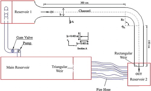
1. Straight input channel: 3.6 m long, located upstream; this length was chosen to create a flow that was stable and developed in the channel before reaching the bend.

2. Curved channel: the central angle of the bend was 90° and the central radius (R_c) was 60.45 cm. The bend was sharp (R_c/b = 1.5 < 3) in terms of channel width (b = 40.3 cm).

3. Straight output channel: 1.8 m long, located downstream; this channel was selected to create flow that developed after the bend and to prevent turbulence caused by overflow upon reaching the bend.

The channel's cross section was 40.3 × 40.3 cm (width× height). The channel boundaries were smooth with a Manning's roughness coefficient (n) of 0.008. The geometric properties of the channel are shown in Figure 1.

Figure 1. Experimental model geometry.

2.2. Experimental process

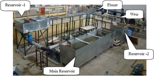
The main reservoir was placed at the beginning of the channel's entrance. A sharp-crested triangular weir in the main reservoir measured the discharge rate, whereas a sharp-crested rectangular weir was installed downstream of the straight channel's end. In order to regulate the channel water depth, the weir height was adjustable. The velocity was read after regulating the discharge rate and water depth within the channel. Upon reading the velocity, the channel bed and water surface values were read for the above-mentioned cross sections with a micrometre. A one-dimensional velocity meter (propeller) was used to read the axial velocities in the flume (Armfield Limited, Co., 1995). A micrometre also measured the water depth. The micrometre measured depth with 0.1 mm precision and velocity with 2 cm/s precision (Akhtari et al., 2009). A view of the channel is presented in Figure 2.

Figure 2. Experimental model scheme.

In the present research, the water entered the flue at five different discharge rates (5, 7.8, 13.6, 19.1 and 25.3 l/s) by changing the opening size of the valve to the main reservoir. The various hydraulic properties applied in the lab are shown in Table 1. The Froude and Reynolds numbers are defined as and , where V is the velocity, g is the gravity acceleration, D is the hydraulic depth, and ν is the kinematic viscosity of .

Table 1. Different experimental hydraulic properties.

Test no.	Normal depth Y (cm)	Discharge rate Q (l/s)	Velocity (m/s)	Froude number	Reynolds number
1	4.5	5	0.273	0.42	12460
2	6	7.8	0.321	0.42	18460
3	9	13.6	0.374	0.40	28940
4	12	19.1	0.394	0.36	36860
5	15	25.3	0.419	0.34	44705

3. Soft computing methods

In this section, the hybrid DT-MLP method is explained. The proposed method comprises MLP ANN regression and a DT classification algorithm.

3.1. Multi-layer perceptron (MLP) neural network

The flexible form of MLP in simulating nonlinear problems with high applicability (Haykin, 1999) has led to the widespread use of this method in practical situations (Chau & Chen, 2006; Kim, Shiri, & Kisi, 2012; Kisi, 2009). An MLP is constructed from three layers: input, hidden and output. The model's input variables are introduced by the input layer via neurons and are then transferred to the hidden layer accordingly (Bishop, 1995). The hidden layer cumulates the input layer neurons by using a weighted summation and subsequently transmits them to a non-linear future via activation functions. MLP models often employ sigmoid activation functions (Chang & Liao, 2012; Ebtehaj & Bonakdari, 2013; Moharrampour, Kherad, Abachi, Zoghi, & Asadi, 2012; Rezaeian Zadeh, Amin, Khalili, & Singh, 2010). Any function that is bounded and has a proportional relation between the input and output variables is a sigmoid function (Smith, 1993). In the present study, the hyperbolic tangent activation function is utilized for the hidden layer (Dawson & Wilby, 2005; Khan & Coulibaly, 2006; Yonaba, Anctil, & Fortin, 2010): (1)

The output MLP layer performs like a linear regressor. Therefore, a weighted summation of the hidden layer neurons is carried out in this layer to evaluate the final model results. The input and output numbers are the same for the neuron layer and model variables, therefore no rule is available to specify the number of hidden layer neurons. If the neuron number is extremely low, the analysis capability and numerical accuracy of prediction will consequently reduce. However, if the hidden layer neuron number is extremely high, the model will undergo overtraining and memorize rather than analyse the data. Thus, trial and error should be employed to determine the number of hidden layers (Bilhan et al., 2010; Gholami et al., 2015; Kisi, 2008b; Kisi & Cigizoglu, 2007). As stated earlier, the hidden and output layers require weighted summations. Determining the weight coefficients in the MLP method is called training. In this study, the Levenberg–Marquardt (LM) method is applied (Levenberg, 1944) for the training process. LM uses the backpropagation algorithm to determine the models’ weights. The training ‘stop’ criterion of the present models is considered 100 epochs, which is when the models converge completely (Kisi, 2008a; Kisi & Cigizoglu, 2007; Zaji & Bonakdari, 2015b). The number of epochs (iterations) is selected with respect to each model. Until both networks reach an acceptable error level between data obtained from the ANN models and experimental data, the training process continues for 100 iterations.

3.2. Hybrid decision-tree-based multi-layer perceptron (DT-MLP) neural network

The hybrid DT-MLP functions with the DT classification algorithm introduced by Breiman, Friedman, Olshen, and Stone (1984) in combination with the MLP regression method in order to increase the method's performance. The class variable Y takes values of 1 to k, where k is the number of determined problem classes. The purpose of classification is to predict Y using the input variables X₁ to X_n, where n is the number of input variables. The DT algorithm has some advantages over other classification methods. The first benefit of DT is its simplicity; DT applies trial and error to find the optimum split locations of the dataset. The second advantage of DT is that its results are presented in a tree structure – thus, presenting classifications of three or more input variables is very convenient.

In the DT-MLP method, a DT is used to optimize the MLP regression method by separating the entire dataset into segments. Therefore, in place of using a large MLP model for the entire dataset, the dataset and MLP are divided into smaller parts. The DT-MLP procedure is as follows. The DT algorithm should be trained with the training dataset. In this step, classification precision plays an important role. High classification precision leads to a large, impractical tree as well as a high probability of overtraining, which occurs when the accuracy of the training dataset classification is better than the testing dataset classification. On the other hand, using smaller trees leads to low classification precision, which consequently results in low DT-MLP regression performance. Therefore, trial and error is employed in the current study to determine the optimum DT classification precision. The DT algorithm splits the dataset into k classes. The maximum allowable number of classes found with trial and error according to the dataset change ranges is selected. Following dataset splitting, the first largest MLP is divided into k smaller MLP models. The maximum number of hidden nodes in the first MLP model is considered equal to the sum of the number of hidden layer neurons in the smaller MLP models, which are developd in the DT-MLP model. Regarding the maximum acceptable number of hidden layer neurons, trial and error is used to find the greatest optimum MLP number and smaller MLP models in the DT-MLP method. There are 12 and 15 hidden layer neurons in the MLP model for velocity and water depth, respectively. To achieve a better comparison of the two models (MLP and DT-MLP), the divisions in the DT-MLP model are considered, while the sum of the hidden layer neurons in the 3 velocity classes and 5 water depths achieved is 12 and 15, respectively, to obtain a model with the highest accuracy. The final step in DT-MLP entails collecting the separate class results of each smaller MLP to generate the final model outcomes. In this stage, the results of the smaller MLP models, which were applied to the classified dataset, are gathered to export the final model results. The most suitable number of classes differs for each dataset case and should be determined using trial and error. In the present study, five different classes, namely ‘very low’, ‘low’, ‘medium’, ‘high’ and ‘very high’ are considered for depth value prediction and three classes of ‘low’, ‘medium’ and ‘high’ are considered for velocity prediction. The DT-MLP procedure is presented in Figure 3. The designed DT-MLP model presents equations for velocity and water surface depth, as shown in Appendices 1 and 2, respectively.

Figure 3. DT-MLP procedure.

3.3. Model performance evaluation

The performance of the MLR, MLP and DT-MLP models in this work is verified with the mean absolute error (MAE), the root mean square error (RMSE), the coefficient of determination (R²) and the average absolute deviation (δ), as computed by the following equations: (2) (3) (4) (5) where is the output observational parameter, is the parameter predicted by the MLP and DT-MLP models, is the mean neural models’ parameter and N is the number of parameters. The RMSE and MAE show the difference between the modeled and observed data in the same unit. Higher model accuracy leads to RMSE and MAE values closer to zero. In order to investigate the performance of the considered models in practical situations with different ranges of input and output variables, non-dimensional statistics are used. δ is the non-dimensional parameter that facilitates the comparison of different models regardless of dimensions and size. A measuring circumstance of observed outcomes replicated by the model is provided by R², which is the linear regression line between the values predicted by the MLP and DT-MLP models and the observed values to determine the network application.

4. Results and discussion

4.1. Data and model analyses

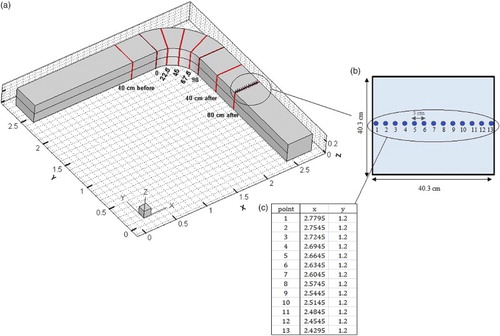
In this section, the data used to train and test the models, the data measurement positions in the experimental tests and the input and output data are explained. The process involved generating two models (MLP and DT-MLP) to predict the velocity and two separate models to predict the water surface depth. Three inputs, i.e., the coordinates of the points in two directions (X and Y) and the flow discharge rate (Q), along with one output, namely the depth-averaged velocity corresponding to these points, are considered in the two velocity prediction models. For the water depth prediction model, the three inputs considered are the coordinates of the points in two directions (X and Y) and the flow discharge rate (Q), along with one output, namely the water depth corresponding to these points. In both velocity prediction models, 104 experimental data were used for each discharge rate, making a total of 520 experimental data for all five discharge rates. These data were divided into two groups: testing and training. Out of 520 data, 364 (70%) were randomly selected for training and 156 (30%) for testing. A total of 506 water surface experimental data were used to predict the water depth, 354 of which (70%) served to train the networks and 152 of which (30%) were used for testing. The data utilized were related to eight different cross sections of a 90° bend (0°, 22.5°, 45°, 67.5°, 90°, 40 cm before the bend and 40 and 80 cm after the bend; Akhtari et al., 2009). Each cross section has 13 transverse points. The value of each velocity data is the depth-averaged velocity of that location. Eight different cross sections, 13 points in the cross section's width, and the distances and coordinates of the studied points are shown in Figure 4.

Figure 4. (a) Three-dimensional view of the cross sections, (b) example of the 13 points in a cross section and (c) example of the point coordinates.

4.2. Evaluation of the models

4.2.1. Velocity prediction

This section presents the results of the depth-averaged velocity predicted by the MLP and DT-MLP models. As mentioned above, three classes, namely ‘low’, ‘medium’ and ‘high’ are considered in the velocity simulation. The classification tree is presented in Figure 5.

Figure 5. DT-MLP velocity classification results.

A comparison of the MLP and DT-MLP results with the experimental values in the training dataset is presented in Figure 6, a careful examination of which reveals that both the ML and DT-MLP models are consistent with the experimental results. However, both models present larger values when predicting the maximum points and smaller values when predicting the minimum points. Both models completely overlap at all points except for the maximum and minimum points. The DT-MLP model predicted the minimum points better than the MLP model. Also, the minimum points completely overlapped with the experimental results of the DT-MLP model. However, both models are alike at the maximum points. A scatter plot graph of the velocity values predicted by the MLP and DT-MLP models is given in Figure 6 against the experimental values from the testing dataset stage. The velocity values are compressed on both sides of the fit line for both models, but the data are scattered more for the MLP model, indicating that the DT-MLP model is more accurate with an R² value close to 1. The DT-MLP hybrid model (R² = 0.9540) is more accurate than the MLP model (R² = 0.9160). It could therefore be stated that using the DT-MLP hybrid algorithm increases the model accuracy when it comes to predicting the flow velocity in a 90° curved channel, as the value of R² is 4% higher.

Figure 6. Comparison of the velocity values predicted by the MLP and DT-MLP models with the experimental values for the training dataset.

The line is fitted to the y = C₁x + C₂ equation, meaning that the model works better when C₁ approaches 1 and C₂ approaches 0. The DT-MLP model has a C₁ value of 0.9540, which is closer to 1 than the C₁ value of the MLP model that is equal to 0.9154. The DT-MLP model indicates the significant difference between the hybrid and MLP models, with a C₂ of 3.28 for DT-MLP. Both models make a slight underestimation. However, the DT-MLP model's amount of underestimation is insignificant and can be overlooked compared with that of the MLP model. Thus, it can be stated that the fit line nearly overlaps the exact line of the DT-MLP model, meaning that the model performed very well.

4.2.2. Water surface prediction

The results for the open-channel bend's water surface are presented in this section. As noted above, the most appropriate number of classes for this dataset is five. Therefore, the dataset is classified using the DT-MLP method into ‘very low’, ‘low’, ‘medium’, ‘high’ and ‘very high’. The optimum classification tree is presented in Figure 7.

Figure 7. DT-MLP water surface.

The scatter plots of the water depth values predicted by each model are drawn in Figure 8 against the experimental values. The water depth predictions for five different discharge rates are separated and drawn on the opposite sides of the corresponding experimental values. It is clear from this figure that the scatter plots of all discharge rates have an R² of 0.9980 with both models, which is almost equal to 1 since the water depths are different for each discharge rate. This indicates that both models (MLP and DT-MLP) predicted water depth highly accurately. The models’ accuracy can, however, be easily compared by breaking each graph down and the results of both models (obtained from one run in each model) are separated for different water depths. The MLP model has the highest accuracy for a discharge rate of 5 l/s with an R² value of 0.9635 and the lowest accuracy for a discharge rate of 19.1 l/s with an R² of 0.9135. The DT-MLP model also benefits from maximum accuracy with a maximum R² value of 0.9724 at a discharge rate of 5 l/s discharge and the lowest accuracy with a minimum R² value of 0.9105 at a discharge rate of 25.3 l/s. Both models performed with maximum accuracy at the minimum discharge rate and minimum accuracy at the maximum discharge rate. The value of R² increased with the DT-MLP model in relation to the MLP model at the discharge rates of 5 and 7.8 l/s, and thus performed better. The value of R² reached 0.9650 with the DT-MLP model from 0.9135 with the MLP model at a discharge rate of 19.1 l/s, therefore R² increased by almost 6% when the hybrid DT-MLP model was used compared with the simple MLP model. Both models performed similarly at the median discharge rate of 13.6 l/s with almost the same R² value. It can therefore be stated that using the hybrid DT-MLP algorithm increases the model accuracy for most discharge rates and leads to higher R² values in comparison to the simple MLP model. This increased accuracy is especially evident at low discharge rates, which is one of the benefits of using hybrid algorithms.

Figure 8. Scatter plot of experimental values with the MLP and DT-MLP models for the test dataset and with separate results relating to each discharge rate for one run.

4.3. Evaluation of depth-averaged velocity profiles

The transverse distributions of depth-averaged velocities in different cross sections at discharge rates of 5, 7.8, 13.6, 19.1 and 25.3 l/s that were predicted by the MLP and DT-MLP models are compared with the corresponding experimental values in Figure 9. The MAEs of these profiles are presented in Table 2. The MLP model error is almost 5 times that of the DT-MLP model at a discharge rate of 25.3 l/s, which indicates that the DT-MLP model is highly accurate and shows an acceptable consistency level with the experimental values in this cross section. The velocity increase is obvious at the entrance cross section of the inner wall bend, which was predicted by all three models for all discharge rates. The accuracy of the DT-MLP model decreased by 45%, 78% and 40% in relation to the MLP model at discharge rates of 5, 7.8 and 25.3 l/s, respectively. The maximum velocity was at the inner wall in the 45° cross section, since the bend under study is a sharp one. Carefully examining the values in the table for this section also reveals that the DT-MLP model performed more successfully at low discharge rates with a 74% accuracy increase compared with the discharge rate of 25.3 l/s and with a 57% decrease in error. At a discharge rate of 5 l/s and in the bend's entrance and middle cross sections, the error value of both models was larger than for the rest of the discharge rates. Therefore, using the DT algorithm to decrease the error in this cross section is one of the most important and fundamental benefits of the hybrid model. The error value of the MLP model is nearly 2.5 times that of the DT-MLP model at discharge rate of 25.3 l/s in the 90° cross section as opposed to the entrance and middle cross sections of the bend, while at the lowest discharge rate of 5 l/s, the error of the DT-MLP model only decreased by 33% in relation to the MLP model (see Figure 9). This is because the MLP and DT-MLP models are unable to predict the return of the velocity profile at the inner wall at low discharge rates. However, only the DT-MLP model is able to predict this at higher discharge rates; therefore, the error value decreases dramatically. The error value of the MLP model is almost 2.3 times that of the DT-MLP model in the cross section located 80 cm after the bend for a discharge rate of 5 l/s. Therefore, it can be generally stated that using the DT-MLP model at low discharge rates decreases the error value by an average of 80% in comparison with the simple MLP model. The DT-MLP model error decreases by an average of 88% at high discharge rates, which is more obvious before and after the end of the bend cross sections. Similar to high and low discharge rates, the error decrease of the DT-MLP model is not as obvious at the three middle discharge rates of 7.8, 13.6 and 19.1 l/s. Therefore, as mentioned previously, using the DT-MLP hybrid algorithm to predict the velocity profile in different cross sections is very effective and efficient in decreasing the error at high and low discharge rates. The DT-MLP equation for predicting the depth-averaged velocity is presented in Appendix 1. According to the equation, the matrix includes 3 rows and 4 columns, where the number of neurons and velocity number in each class are 4 and 3, respectively. Hence, there are a total of 12 neurons for velocity.

Figure 9. Transverse distribution of depth-averaged velocity for the MLP and DT-MLP models compared with the experimental values at different discharge rates.

Table 2. MAE error values of the velocity transverse profile for the MLP and DT-MLP models at different discharge rates and cross sections.

	Q = 5		Q = 7.8		Q = 13.6		Q = 19.1		Q = 25.3
	MLP	DT-MLP	MLP	DT-MLP	MLP	DT-MLP	MLP	DT-MLP	MLP	DT-MLP
40 cm before	1.014	0.56	1.39	1.28	0.88	0.7	1.25	0.99	2.58	0.53
0°	1.89	1.058	1.38	0.95	1.2	1.04	1.52	2.11	1.72	1.24
45°	1.9	1.09	1.36	1.25	1.33	0.97	1.23	1.05	1.86	1.18
90°	2.72	2.03	2.61	2	2.2	1.32	2.84	1.88	3.3	1.51
40 cm after	1.43	0.64	1.49	1.37	1.015	0.99	1.1	1.046	1.24	1.23
Averaged	1.8	1	1.446	1.37	1.325	1	1.6	1.41	2.14	1.14

4.4. Evaluation of water surface profiles

The transverse distribution of the water surface transverse cross section is compared with the corresponding experimental values in Figure 10 at the cross sections of 0°, 45°, 90° and 40 cm after the bend under different discharge rates. The MAEs of these profiles are presented in Table 3. The MLP and DT-MLP models were both run once for all discharge rates. However, in order to compare them better and more precisely with regard to Table 4 and since the water surface prediction models performed similarly, the results related to each discharge rate were separated and the models were evaluated. The presence of centrifugal force (due to the channel's curve) in the initial bend of the cross section creates a transverse gradient in the water surface such that the flow depth increases at the outer wall and decreases at the inner wall. It is clear that both models can efficiently predict the free-surface profile at the channel cross section entrance under all discharge rates. According to Table 3, the DT-MLP model exhibited a 67% error decrease compared with the MLP model in this cross section at a discharge rate of 5 l/s and thus is more consistent with the experimental results. The DT-MLP model was more accurate than the MLP model at a discharge rate of 7.8 l/s and its error decreased by 65%. Both models performed alike at the median discharge rate of 13.6 l/s and the DT-MLP model had a slightly greater error value. DT-MLP was again more accurate than MLP at discharge rates of 19.1 and 25.3 l/s with a 50% and 144% error decrease, respectively. It can be stated that the DT-MLP model results are more compatible with the experiments at the entrance bend cross section for all discharge rates, with an average error decrease of 61% compared with the results of the MLP model. The water surface gradient is also visible in the profiles of the following cross sections, and the water is deeper at the channel's outer wall than the inner wall. Both models performed quite similarly for the cross section in the middle of the bend while the DT-MLP model had a slight error decrease compared with the MLP model. The DT-MLP model performed much better than the simple MLP model at the end cross section, signifying a noticeable error decrease. The error value of the DT-MLP model decreased by 162.5%, 22.5%, 40%, 180% and 10% for the discharge rates of 5, 7.8, 13.6, 19.1 and 25.3 l/s, respectively, in relation to the MLP model. The accuracy of the DT-MLP model increased by an average of 83% in the end cross section compared with the MLP model. The water surface had not yet become stable after the bend exit due to secondary flow. The secondary flow gradually faded away in the cross section located 40 cm after the bend as well as in farther cross sections, and the flow depth reached its initial value (the normal channel depth). In the section 40 cm after the bend, the MAE value reached 0.011 with the DT-MLP model at a discharge rate of 5 l/s compared to 0.025 with the MLP model, signifying a 127% decrease. The error of the DT-MLP model decreased by an average of approximately 31.5% in the section 40 cm after the bend for all discharge rates in comparison with the MLP model. It can generally be stated that the error values of the DT-MLP model decreased by 60%, 21%, 14.5%, 83% and 45% for discharge rates of 5, 7.8, 13.6, 19.1 and 25.3 l/s, respectively, in comparison with the MLP model. The error decrease of the DT-MLP model is more pronounced at high and low discharge rates in all cross sections than for the middle discharge rates. The maximum error decrease in the DT-MLP model is 162.5% and 180% at the discharge rates of 5 and 19.1 l/s, respectively, at the cross section at the end of the bend. It can be concluded that using the suggested modified model to predict water depth in channels in order to better execute them and design wall heights correctly is quite practical. The DT-MLP equation for water surface simulation is presented in Appendix 2. In this equation, the matrix has 3 rows and 3 columns, meaning the numbers of neurons and water depth in each class are 3 and 5, respectively. Therefore, there are a total of 15 neurons for depth.

Figure 10. The transverse profile of water surface predicted by the MLP and DT-MLP models compared with the experimental results at different discharge rates at cross sections of (a) 0°, (b) 45°, (c) 90° and (d) 40 cm after the bend.

Table 3. MAE error values of the water surface transverse profile for the MLP and DT-MLP models at different discharge rates and cross sections.

	Q = 5		Q = 7.8		Q = 13.6		Q = 19.1		Q = 25.3
	MLP	DT-MLP	MLP	DT-MLP	MLP	DT-MLP	MLP	DT-MLP	MLP	DT-MLP
0°	0.035	0.021	0.038	0.023	0.024	0.026	0.044	0.018	0.09	0.06
45°	0.025	0.035	0.041	0.032	0.046	0.046	0.031	0.025	0.057	0.05
90°	0.042	0.016	0.055	0.045	0.07	0.05	0.084	0.03	0.11	0.055
40 after	0.025	0.011	0.024	0.034	0.02	0.014	0.06	0.048	0.04	0.042
Averaged	0.032	0.02	0.04	0.033	0.04	0.035	0.055	0.03	0.074	0.051

Table 4. Evaluation of the MLR, MLP and DT-MLP models in terms of velocity and water depth prediction with the testing dataset.

	Velocity prediction				Water depth prediction
	RMSE	MAE	R^2	δ(%)	RMSE	MAE	R^2	δ(%)
MLP	2.40	1.76	0.91	4.60	0.054	0.040	0.99	0.035
DT-MLP	2.20	1.52	0.92	3.96	0.058	0.042	0.99	0.036
MLR	5.46	4.28	0.50	77.91	0.295	0.235	0.85	0.945

4.5. Comparison of models’ capabilities

The performance of the MLP and DT-MLP models used to predict the depth-averaged velocity and water surface is presented in Table 4 through the RMSE, MAE, R² and δ (%) statistical indexes. The two parameters predicted by the MLR model are also included, and the model's performance compared to the MLP and DT-MLP models is evaluated. The values show that the MLP and DT-MLP models predicted the velocity with an R² of 0.9200 and 0.9200, which are higher than the value obtained with the MLR model (0.5). The R² value of the MLR model in predicting water surface depth is smaller than that of the two other models. The MLP and DT-MLP models predicted both velocity and flow depth more accurately than the MLR model.

The values in Table 4 thus indicate that both the MLP and DT-MLP models predicted flow velocity accurately. The DT-MLP model (RMSE = 2.2) outperformed the MLP model (RMSE = 2.4) in velocity prediction. δ reached 3.96 with DT-MLP from 4.6 with MLP, while the deviation of the DT-MLP model decreased by approximately 16% in relation to the MLP model. Both models performed very well, with an R² of 0.9900 (almost 1) in water depth prediction. This R² value is related to each model's results for all discharge rates. When separating the results related to one run (Figure 8), the R² variables were in the 0.9 to 1 range. In general, however, the DT-MLP model (RMSE = 0.058) outperformed the MLP model (RMSE = 0.054).

Figure 11 illustrates the bar graph of MAE error values with both the MLP and DT-MLP models in predicting velocity and water depth at different discharge rates with the test dataset. The MAEs are drawn for the MLP and DT-MLP models on the vertical axes of these graphs. Generally, viewing these graphs clarifies that the error value is smaller for the water depth prediction model Figure 11(a) than for the velocity prediction model Figure 11(b); therefore, it can be stated that both the MLP and DT-MLP models performed well in predicting water depth. The graph in Figure 11(a), water surface prediction, shows that the error value of the DT-MLP model significantly decreases at the discharge rates of 7.8 and 19.1 l/s compared with the MLP model. This error value decreases at a discharge rate of 5 l/s with the DT-MLP model; however, since both the MLP and DT-MLP models performed well at this discharge rate, the error value is very small and invisible on the graph. Both models performed quite similarly at discharge rate of 13.6 l/s and the MLP model had a smaller error value at discharge rate of 25.3 l/s.

Figure 11. The MAE error bar graph for the MLP and DT-MLP models with the test dataset at different discharge rates for predicting (a) water surface depth and (b) velocity.

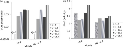
The error decrease is very noticeable in Figure 11(b), velocity prediction, for the graphs for the DT-MLP model rather than the MLP model at all discharge rates. The decreasing error value of DT-MLP is especially noticeable at the low discharge rate of 5 l/s, similar to the water depth prediction model. This may be considered one of the advantages of the present research in terms of using the DT-MLP algorithm to decrease the error in shallow water (approaching supercritical flow) of both velocity and water depth prediction models. Comparing Figure 11(a) and (b), it can be seen that the DT-MLP hybrid algorithm is more successful when employed in models that predict velocity rather than depth. Because the error value decrease is so tangible at higher as well as lower discharge rates in these models, the velocity prediction of the DT-MLP model in the present research is effective and successful for all discharge rates. Using the proposed DT-MLP hybrid model in the present study is therefore very effective in practical cases.

5. Conclusion

An attempt was made in the present research to evaluate the performance of an MLP model in predicting velocity and water surface variables in a 90° bend before and after the model was combined with a decision tree (MLP vs. DT-MLP). A simple MLP model was also designed to test the suggested model and then both were compared. A total of 520 and 506 depth-averaged velocity and water surface experimental samples were used for training and testing the networks at five different discharge rates. The performance of the two models was examined and compared with the MLR and experimental results. In velocity and water surface depth prediction, the MLP and DT-MLP models exhibited lower error than the MLR model. The results indicate that the DT-MLP model (MAE = 1.76) performed better in predicting flow velocity than the MLP model (MAE = 1.52). The DT-MLP model accuracy was greater than the MLP model in flow depth prediction as well, with significant reduction in model error. According to the model results comparison for different flow discharge rates, the DT-MLP model was substantially more accurate compared to the MLP model at high and low discharge rates (5 and 19.1 l/s) rather than other discharge rates. Therefore, using the DT-MLP hybrid algorithm proposed in the current research decreases the simple MLP model's error to a large degree and can be used in practical cases. Other soft computing methods in combination with a DT model can be used to predict various additional flow variables in bends, for instance shear stress, pressure and turbulence intensity.

Acknowledgments

The authors would like to express their appreciation to anonymous reviewers for their helpful comments.

Disclosure statement

No potential conflict of interest was reported by the authors.

Appendix 1. DT-MLP equation for velocity prediction

The matrix row numbers represent the numbers of model inputs (inputs: X, Y, Q). The column numbers signify the numbers of neurons used in each class. There are 12 hidden layer neurons for the velocity prediction models.

For the ‘low’ class:

For the ‘medium’ class:

For the ‘high’ class:

Appendix 2. DT-MLP equation for water surface prediction

The matrix row numbers represent the numbers of model inputs (inputs: X, Y, Q). The column numbers signify the numbers of neurons used in each class. There are 15 hidden layer neurons for the flow depth prediction model.

For the ‘very low’ class:

For the ‘low’ class:

For the ‘medium’ class:

For the ‘high’ class:

For the ‘very high’ class:

References

- Akbari, M., Solaimani, K., Mahdavi, M., & Habibnejhad, M. (2011). Monitoring of regional low-flow frequency using artificial neural networks. Journal of Water Sciences Research, 3(1), 1–17.
- Akhtari, A. A., Abrishami, J., & Sharifi, M. B. (2009). Experimental investigations water surface characteristics in strongly-curved open channels. Journal of Applied Sciences, 9(20), 3699–3706. doi: 10.3923/jas.2009.3699.3706
- Anwar, H. O. (1986). Turbulent structure in a river bend. Journal of Hydraulic Engineering, 112(8), 657–669. doi: 10.1061/(ASCE)0733-9429(1986)112:8(657)
- Armfield Limited, Co. (1995). Instruction manual of miniature propeller velocity meter type H33.
- Baghalian, S., Bonakdari, H., Nazari, F., & Fazli, M. (2012). Closed-form solution for flow field in curved channels in comparison with experimental and numerical analyses and artificial neural network. Engineering Applications of Computational Fluid Mechanics, 6(4), 514–526. doi: 10.1080/19942060.2012.11015439
- Bahrami, E. J., Ghaneeizad, S. M., & Akhtari, A. A. (2009). Experimental study on flow structure in strongly curved open channel 90-degree bends. International Symposium on Water Management and Hydraulic Engineering. (A32). Ohrid, Macedonia, Greece, 1–5 September.
- Bergs, M. A. (1990). Flow processes in a curved alluvial channel. Ph. D. Thesis. The University of Iowa.
- Bilhan, O., Emiroglu, M. E., & Kisi, O. (2010). Application of two different neural network techniques to lateral outflow over rectangular side weirs located on a straight channel. Advances in Engineering Software, 41(6), 831–837. doi: 10.1016/j.advengsoft.2010.03.001
- Bilhan, O., Emiroglu, M. E., & Kisi, O. (2011). Use of artificial neural networks for prediction of discharge coefficient of triangular labyrinth side weir in curved channels. Advances in Engineering Software, 42(4), 208–214. doi: 10.1016/j.advengsoft.2011.02.006
- Bishop, C. M. (1995). Neural networks for pattern recognition. NewYork, NY: Oxford university press Inc.
- Blanckaert, K., & DeVriend, H. J. (2004). Secondary flow in sharp open-channel bends. Journal of fluid Mechanics, 498, 353–380. doi: 10.1017/S0022112003006979
- Blanckaert, K., & Graf, W. H. (2001). Mean flow and turbulence in open channel bend. Journal of Hydraulic Engineering, 127(10), 835–847. doi: 10.1061/(ASCE)0733-9429(2001)127:10(835)
- Bodnar, T., & Prihoda, J. (2006). Numerical simulation of turbulent free-surface flow in curved channel. Flow, Turbulence and Combustion, 76, 429–442. doi: 10.1007/s10494-006-9030-x
- Bonakdari, H., Baghalian, S., Nazari, F., & Fazli, M. (2011). Numerical analysis and prediction of the velocity field in curved open channel using artificial neural network and genetic algorithm. Engineering Applications of Computational Fluid Mechanics, 5(3), 384–396. doi: 10.1080/19942060.2011.11015380
- Breiman, L., Friedman, J. H., Olshen, R. A., & Stone, C. J. (1984). Classification and regression trees. Wadsworth, Belmont, California, USA: Belmont, Wadsworth international group.
- Chang, C. L., & Liao, C. S. (2012). Parameter sensitivity analysis of artificial neural network for predicting water turbidity. World Academy of Science, Engineering and Technology, 70, 657–660.
- Chau, K. W., & Chen, W. (2006). Real-time prediction of water stage with artificial neural network approach. Lecture Notes in Computer Science, 2557, 715. doi: 10.1007/3-540-36187-1_64
- Chau, K.W., & Wu, C. L. (2010). A hybrid model coupled with singular spectrum analysis for daily rainfall prediction. Journal of Hydroinformatics, 12 (4), 458–473. doi: 10.2166/hydro.2010.032
- Chau, K. W., Wu, C. L., & Li, Y. S. (2005). Comparison of several flood forecasting models in Yangtze river. Journal of Hydrologic Engineering, 10(6), 485–491. doi: 10.1061/(ASCE)1084-0699(2005)10:6(485)
- Cheng, C., Chau, K. W., Sun, Y., & Lin, J. (2005). Long-term prediction of discharges in manwan reservoir using artificial neural network models. Lecture Notes in Computer Science, 3498, 1040–1045. doi: 10.1007/11427469_165
- Chen, W., Chau, K. W. (2006). Intelligent manipulation and calibration of parameters for hydrological models. International Journal of Environment and Pollution, 28(3–4), 432–447. doi: 10.1504/IJEP.2006.011221
- Dawson, C. W., & Wilby, R. L. (2005). Hydrological modelling using artificial neural networks. Progress in physical geography, 25(1), 80–108. doi: 10.1177/030913330102500104
- DeMarchis, M., & Napoli, E. (2006). 3D numerical simulation of curved open channel flows. Proceedings of 6th International Conference on Water Resources, Hydraulics & Hydrology (pp. 86–91). Chalkida, Evia Island, Greece, May 11–13.
- DeVriend, H. J., & Geldof, H. J. (1983). Main flow velocity in short river bends. Journal of Hydraulics Engineering, 109(7), 991–1011. doi: 10.1061/(ASCE)0733-9429(1983)109:7(991)
- Dursun, O. F., Kaya, N., & Firat, M. (2012). Estimating discharge coefficient of semi-elliptical side weir using ANFIS. Journal of Hydrology, 426-427, 55–62. doi: 10.1016/j.jhydrol.2012.01.010
- Ebtehaj I., & Bonakdari, H. (2013). Evaluation of sediment transport in sewer using artificial neural network. Engineering Applications of Computational Fluid Mechanics, 7(3), 382–392. doi: 10.1080/19942060.2013.11015479
- Gholami, A., Akhtari, A. A., Minatour, Y., Bonakdari, H., & Javadi, A. A. (2014). Experimental and numerical study on velocity fields and water surface profile in a strongly-curved 90° open channel bend. Engineering Applications of Computational Fluid Mechanics, 8(3), 447–461. doi: 10.1080/19942060.2014.11015528
- Gholami, A., Bonakdari, H., Zaji, A. H., & Akhtari, A. A. (2015). Simulation of open channel bend characteristics using computational fluid dynamics and artificial neural networks. Engineering Applications of Computational Fluid Mechanics, 9(1), 355–369. doi: 10.1080/19942060.2015.1033808
- Haykin, S. (1999). Neural networks. A comprehensive foundation, 2nd ed. Englewood Cliffs, NJ: Prentice-Hall Inc.
- Jeng, D. S., Bateni, S. M., & Lockett, E. (2005). Neural Network assessment for scour depth around bridge piers. The University of Sydney, Environmental Fluids, Research Report No R855.
- Jung, J. W., & Yoon, S. E. (2000). Flow and bed topography in a 180-degree curved channel. 4th International Conference on Hydro-Science and Engineering: Korea Water Resources Association.
- Khan, M. S. & Coulibaly, P. (2006). Application of support vector machine in lake water level prediction. Journal of Hydrologic Engineering, 11(3), 199–205. doi: 10.1061/(ASCE)1084-0699(2006)11:3(199)
- Kim, S., Shiri, J., & Kisi, O. (2012). Pan evaporation modeling using neural computing approach for different climatic zones. Water Resources Management, 26, 3231–3249. doi: 10.1007/s11269-012-0069-2
- Kisi, O. (2008a). Multi-layer perceptrons with Levenberg-Marquardt training algorithm for suspended sediment concentration prediction and estimation. Hydrological Sciences Journal, 49(6), 1025–1040.
- Kisi, O. (2008b). The potential of different ANN techniques in evapotranspiration modelling. Hydrological Processes, 22, 2449–2460. doi: 10.1002/hyp.6837
- Kisi, O. (2009). Daily pan evaporation modelling using multi-layer perceptrons and radial basis neural networks. Hydrological Processes, 23, 213–223. doi: 10.1002/hyp.7126
- Kisi, O., & Cigizoglu, H. K. (2007). Comparison of different ANN techniques in river flow prediction. Civil Engineering and Environmental Systems, 24(51), 211–231. doi: 10.1080/10286600600888565
- Kisi, O., Emiroglu, M. E., Bilhan, O., & Guven, A. (2012). Prediction of lateral outflow over triangular labyrinth side weirs under subcritical conditions using soft computing approaches. Expert Systems with Applications, 39(3), 3454–3460. doi: 10.1016/j.eswa.2011.09.035
- Leschziner, M. A., & Rodi, W. (1979). Calculation of strongly curved open channel flow. Journal of the Hydraulics Division, 105(10), 1297–1314.
- Levenberg, K. (1944). A method for the solution of certain non-linear problems in Least-Squares. The Quarterly of Applied Mathematics, 2, 164–168.
- Mohamed, H. I., & Hashem, M. (2006). Estimation of longitudinal dispersion coefficient in rivers using artificial neural networks. Journal of Engineering Sciences, 34(5), 1341–1352.
- Moharrampour, M., Kherad, M., Abachi, N., Zoghi, M., & Asadi, M. R. A. A. (2012). Comparison of artificial neural networks ANN and statistics in daily flow forecasting. Advances in Enviromental Biology, 6(2), 863–868.
- Naji, M. A., Ghodsian, M., Vaghefi, M., & Panahpur, N. (2010). Experimental and numerical simulation of flow in a 90° bend. Flow Measurement and Instrumentation, 21(3), 292–298. doi: 10.1016/j.flowmeasinst.2010.03.002
- Ramamurthy, A., Han, S., & Biron, P. (2013). Three-dimensional simulation parameters for 90° open channel bend flows. Journal of Computing in Civil Engineering, 27(3), 282–291. doi: 10.1061/(ASCE)CP.1943-5487.0000209
- Rezaeian Zadeh, M., Amin, S., Khalili, D., & Singh, V. P. (2010). Daily outflow prediction by multilayer perception with logistic sigmoid and tangent sigmoid activation functions. Journal of Water Resources Mangement, 24(11), 2673–2688. doi: 10.1007/s11269-009-9573-4
- Rowiński, P. M., Piotrowski, A., & Napiórkowski, J. J. (2005). Are artificial neural network techniques relevant for the estimation of longitudinal dispersion coefficient in rivers?/Les techniques de réseaux de neurones artificiels sont-elles pertinentes pour estimer le coefficient de dispersion longitudinale en rivières? Journal of Hydrological Sciences, 50(1), 175–187. doi: 10.1623/hysj.50.1.175.56339
- Rozovskii, I. L. (1957). Flow of Water in Bends of Open Channels. Kiev: Academy of Sciences of the Ukrainian SSR. [Jerusalem: Israel Program for Scientific Translations [1961]].
- Sahu, M., Jana, S., Agarwal, S., & Khatua, K. K. (2011). Point form velocity prediction in meandering open channel using artificial neural network. 2nd International Conference on Environmental Science and Technology: Vol. 6. (pp. 209–212). Singapore: IACSIT Press.
- Shukry, A. (1950). Flow around bends in an open flume. Transactions, ASCE, 115, 751–788.
- Smith, M. (1993). Neural networks for statistical modeling. NewYork, NY: Thomson Learning.
- Sui, J., Fang, D., & Karney, B. W. (2006). An experimental study into local scour in a channel caused by a 90° bend. Canadian Journal of Civil Engineering, 33, 902–911. doi: 10.1139/l06-037
- Taormina, R., & Chau, K. W. (2015). Neural network river forecasting with multi-objective fully informed particle swarm optimization. Journal of Hydroinformatics, 17(1), 99–113. doi: 10.2166/hydro.2014.116
- Tayfur, G. (2002). Artificial neural network for sheet sediment transport. Hydrological Sciences Journal- Journal des Science Hydrologiques, 47(6), 879–892. doi: 10.1080/02626660209492997
- Uddin, M. N., & Rahman, M. M. (2012). Flow and erosion at a bend in the braided Jamuna River. International Journal of Sediment Research, 27(4), 498–509. doi: 10.1016/S1001-6279(13)60008-6
- Wang, W. C., Chau, K. W., Cheng, C. T., & Qiu, L. (2009). A comparison of performance of several artificial intelligence methods for forecasting monthly discharge time series. Journal of Hydrology, 374(3–4), 294–306. doi: 10.1016/j.jhydrol.2009.06.019
- Wang, W. C., Chau, K. W., Xu, D. M., & Chen, X. Y. (2015). Improving forecasting accuracy of annual runoff time series using ARIMA based on EEMD decomposition. Water Resources Management, 29(8), 2655–2675. doi: 10.1007/s11269-015-0962-6
- Wu, C. L., Chau, K. W., & Li, Y. S. (2008). River stage prediction based on a distributed support vector regression. Journal of Hydrology, 358(1–2), 96–111. doi: 10.1016/j.jhydrol.2008.05.028
- Wu, C. L., Chau, K. W., & Li, Y. S. (2009). Methods to improve neural network performance in daily flows prediction. Journal of Hydrology, 372(1–4), 80–93. doi: 10.1016/j.jhydrol.2009.03.038
- Ye, J., & McCorquodale, J. A. (1998). Simulation of curved open channel flows by 3D hydrodynamic model. Journal of Hydraulic Engineering, 124(7), 687–698. doi: 10.1061/(ASCE)0733-9429(1998)124:7(687)
- Yonaba, H., Anctil, F., & Fortin, V. (2010). Comparing sigmoid transfer functions for neural network multistep ahead streamflow forecasting. Journal of Hydrologic Engineering, 15(4), 275–283. doi: 10.1061/(ASCE)HE.1943-5584.0000188
- Zaji, A. H., & Bonakdari, H. (2014). Performance evaluation of two different neural network and particle swarm optimization methods for prediction of discharge capacity of modified triangular side weirs. Flow Measurement and Instrumentation, 40, 149–156. doi: 10.1016/j.flowmeasinst.2014.10.002
- Zaji, A. H., & Bonakdari, H. (2015a). Application of artificial neural network and genetic programming models for estimating the longitudinal velocity field in open channel junctions. Flow Measurement and Instrumentation, 41, 81–89. doi: 10.1016/j.flowmeasinst.2014.10.011
- Zaji, A. H., & Bonakdari, H. (2015b). Efficient methods for prediction of velocity fields in open channel junctions based on the artifical neural network. Engineering Applications of Computational Fluid Mechanics, 9(1), 1–13. doi: 10.1080/19942060.2015.1004821
- Zeng, Y., & Huai, W. (2009). Application of artificial neural network to predict the friction factor of open channel flow. Communications in Nonlinear Science and Numerical Simulation, 14, 2373–2378. doi: 10.1016/j.cnsns.2007.12.012
- Zhang, M. L., & Shen, Y. M. (2008). Three dimensional simulation of meandering river based on 3-D k-ε (RNG) turbulence model. Journal of Hydrodynamics, 20(4), 448–455. doi: 10.1016/S1001-6058(08)60079-7