Numerical simulation of the flow through a compressor-valve model using an immersed-boundary method

ABSTRACT

Hermetic reciprocating compressors are widely used in small- and medium-size refrigeration systems based on the vapor-compression cycle. One of the main parts of this type of compressor is the automatic valve system used to control the suction and discharge processes. As the suction and discharge losses represent a large amount of the total thermodynamic losses (47%), a small improvement in the suction and discharge processes can produce expressive increases in the thermodynamic efficiency of the compressor. In this work, a new numerical methodology is applied to solve the flow through reed-type valves. The numerical results were experimentally validated through the pressure distribution acting on the frontal disk of a radial diffuser, which is a geometry usually used to model this type of valve. The numerical results for the velocity and pressure fields were comprehensively explored during the opening and closing movement imposed to the reed. The good quality of these results show that the numerical methodology is very promising in terms of solving the flow in the actual dynamics of reed-type valves.

KEYWORDS:

• Compressor valve
• immersed boundary: adaptive refinement

1. Introduction

Hermetic reciprocating compressors are widely used in small- and medium-size refrigeration systems based on the vapor compression cycle. One of the main parts of this type of compressor is the automatic valve system used to control the suction and discharge processes. According to Ribas, Deschamps, Fagotti, Morriesen, and Dutra (2008), the thermodynamic efficiency in a high-efficiency refrigeration compressor operating with refrigerant R134a is about 80 to 83%. They divided the thermodynamic losses into leakage losses (4%), superheating losses (49%), and suction and discharges losses (47%). As the suction and discharge losses represent a large amount of the total thermodynamic losses, a small improvement in the suction and discharge processes can produce expressive increases in the thermodynamic efficiency.

In order to improve the suction and discharge processes, it is necessary to study the flow through the suction and discharge valves. Studying the flow through these valves can help to determine the main parameters that influence the flow (orifice diameter, shape and dimensions of the reed, Reynolds number, and force acting on the reed) and how these parameters relate to each other. The valve system can then be optimized in order to reduce the losses caused by the friction forces of the flow (entropy generation), which would permit a larger amount of refrigerant to flow into the cylinder and be compressed by the whole compressor system. As a final result this would represent an increase in compressor efficiency.

In this type of compressor, the valves must be as simple as possible to reduce manufacturing cost. Thus, the valve system is usually designed to operate without any device to control the movement of the valve. Therefore, valves are usually just thin beans (reeds) fixed on one edge. The movement of the reed is caused by the forces of the flow acting on its surfaces and the structural response of the reed. Then, physical properties of the flow and physical parameters of the reed (mass, damping, and stiffness) influence the behavior of the system. This is a typical problem of fluid structure interaction, in which the fluid flow through the valve system is very difficult to predict due to its high complexity.

The majority of prior numerical simulation studies (Colaciti, López, Navarro, & Cabezas-Gmez, 2007; Ferreira, Deschamps, & Prata, 1989; Mariani, Prata, & Deschamps, 2010; Possamai, Ferreira, & Prata, 2001; Prata, Pilichi, & Ferreira, 1995) have considered reed valves as circular disks without taking into account the fluid structure interaction – that is, the circular disks have been considered static. Pereira, Santos, Deschamps, and Kremer (2012) have also modeled the reed as a circular disk but introduced the one-dimensional mass-spring-damper model in order to obtain the movement of the disk.

A few works have used actual geometries for modeling valve-reed dynamics. The finite-element method was used by Machu, Albrecht, Bielmeier, Daxner, and Steinruck (2004) to obtain the movement of an actual reed valve by using a simplified lumped model for calculating the force acting on the surface of the reed – that is, they have not solved the fluid flow problem through the valve. An approach to the problem of reed dynamics by using an actual geometry for the valve was presented by Kim, Ahn, and Kim (2008). The authors solved the fluid structure interaction problem by using commercial software in which an Arbitrary Lagangian Eulerian formulation was used to solve the problem. However, the numerical methodology is not presented in detail and the flow behavior is not explored. Apparently, Kinjo, Nakano, Hikichi, and Morinishi (2010) have also solved the fluid structure interaction problem in reed-type valves considering an actual geometry. They used the virtual flux method to capture the reed movement. As with Kim et al. (2008), the authors do not present enough details about their numerical methodology and do not explore the characteristics of the flow. Commercial software was used by Mistry, Bhakta, Dhar, Bahadur, and Dey (2012) to obtain the dynamics of an actual reed valve but again the authors do not present the numerical methodology used to solve the fluid structure interaction and, as with the other two studies, have not analyzed the fluid flow.

Based on the reviewed literature, it is clear that the problem of fluid structure interaction in actual geometries of reed-type valves usually used in refrigeration compressors still requires further research in order to develop and test new numerical methodologies to treat the interaction of the dynamics of the structure and flow field. The objective of this work is to apply a new methodology for solving the problem of presenting the fluid structure interaction of the flow through reed-type valves. An actual geometry usually used in suction valves is used for modeling the reed. The numerical methodology is experimentally validated and presented in detail, along with results for velocity and pressure fields for several configurations of the flow. The results show that the numerical methodology is appropriate for solving the problem.

2. Numerical methodology

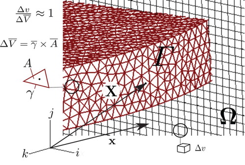
Considering the unsteady, isothermal and incompressible flow of a Newtonian fluid, the equations that must be solved to obtain the pressure and velocity fields of the flow are the continuity and momentum equations: (1) (2) where u is the velocity vector field, p is the pressure field, ρ and µ are the density and absolute viscosity, respectively, and f is the density field of any type of body force (Eulerian force). In this methodology, this Eulerian force represents the force of the flow acting on the surface of any solid body immersed in the flow. As a response to this force, the body reacts with another force known as the Lagrangian interfacial force, F, in such way that the velocity of the flow on the surface of the body acquires the same velocity as the body. If the body is at rest, the velocity of the fluid on its surface is zero in order to comply with the no-slip condition of the flow on the surface. Therefore, the Lagrangian interfacial force is used to identify the boundary of the body. The Eulerian density force (f) is determined by distributing the Lagrangian force to the Eulerian cells close to the boundary with the equation (3) where x is the position vector of the Eulerian cell, X is the position vector of the Lagrangian point, ΔV is the discrete volume defined for each Lagrangian point, D is the distribution function with Gaussian function properties, and Γ is the Lagrangian domain. The present method is based on the immersed-boundary method (Peskin, 1973), which relies on the Dirac delta for the calculation of f. As it is not possible to discretize the Dirac delta, the discrete function D is used. Figure 1 shows the meaning of the main parameters. In this work, capital letters refer to Lagrangian variables and lowercase letters refer to Eulerian variables.

Figure 1. The Lagrangian and Eulerian domains.

Several models developed to calculate the Lagrangian interfacial force can be found in Mittal and Iaccarino (2005). In the present work, the model proposed by Wang, Fan, and Luo (2008) is used for the Lagrangian density force calculations. In this method the direct forcing process, which is normally used in other methodologies, is applied several times on the Eulerian cells located at the vicinity of the immersed boundary until the velocity field evaluation represents the boundary velocity value as expected – in this case, the no-slip condition. Since this method applies direct forcing several times, it is named multi-direct forcing and its steps are as follows.

First, evaluation of the Eulerian velocity on the Lagrangian point with the distribution function: (4)

Second, calculus of the Lagrangian force density F for the iteration: (5)

Third, distribution of the Lagrangian force density to the Eulerian cells: (6)

Fourth, update the velocity field after forcing: (7)

In Equation (5(5) ), U^t+Δt represents the velocity condition on the immersed boundary. These four actions are cycled until U^t+Δt = Uⁱ. Then, the total force on the immersed boundary can be determined by (8) where N is the number of multi-direct forcing cycles.

A structured adaptive mesh refinement (SAMR) strategy is used for local refinement in regions where fine resolution is required. According to Alvarez (2013), SAMR is relatively easy to implement compared with other adaptive refinement methods and provides the convenience of using the same discretization of uniform Cartesian grids, including the easy access of cells and vicinity. The mesh is composed of a sequence of nested blocks (Figure 2(a)) and it is possible to verify that there are different refinement levels. In the case of Figure 2(a), there are three refinement levels, and this mesh is commonly referred to as a 6 × 6L3 –a base grid of 6 × 6 and three refinement levels (including the base level).

Figure 2. Comparison of (a) properly and (b) improperly nested meshes.

Two rules must be attended to in order to consider the mesh block as appropriately nested. Figure 2 shows an example of a bi-dimensional SAMR mesh to demonstrate these rules, which are defined as follows:

• At least one cell from a level L must separate blocks from levels L + 1 and L − 1.

• The corners of a block from a level L must coincide with the corners of cells from a coarser level L − 1.

In Figure 2(a) the blocks are appropriately nested, while Figure 2(b) exemplifies violations of the rules described above. The communications of the grid blocks with the vicinity is made with a layer of ghost cells around each block, and the ghost values are determined by the location of the ghost cell; if the ghost cell touches the domain boundary, the boundary conditions determine the ghost cell value; if the cell is inside the domain on a fine or coarse interface then interpolations are accomplished to determine its value, and if the ghost cell is located in the same place as another cell of the same level (from another block) then the value of the cell is injected into the ghost cell. More details about ghost cell calculations can be found in Nós (2007), Villar (2007), Lima (2012), and Alvarez (2013).

The strategy for refining the domain is based on the position of the immersed boundary and the magnitude of the vorticity field. The finest level is set for the regions near the Lagrangian points, while the refinement level for the rest of the domain is set according to the local magnitude of the vorticity field. Figure 3 shows an example of a body modeled on the basis of the Lagrangian domain being covered by the finest level of the Eulerian domain.

Figure 3. Lagrangian mesh covered by Eulerian refinement blocks.

The classic Smagorinsky (1963) sub-grid model is used to represent the turbulent kinetic energy transfer in the eddies of the turbulent flow. This model is based on the Boussinesq hypothesis and relies on the concept of turbulent viscosity for the closure (modeling of additional stresses) of the filtered Navier–Stokes equations. This model belongs to a class of models denominated as large eddy simulation (LES), where the Navier–Stokes equations are filtered by the spatial grid. This filtering process separates the eddies into large eddies – which can be represented by the grid resolution – and small eddies which cannot, due to its prohibitive small scale. While the large eddies are calculated by the numerical simulations, the small-eddy effects are introduced as an additional turbulent viscosity field which is added to the molecular viscosity field. In the Smagorinsky model, the turbulent viscosity is calculated as a function of the rate of strain tensor S and the Smagorinsky constant Cs, taken to be 0.2 in the present simulations. Equation (9(9) ) shows the equation for the turbulent viscosity calculation: (9) The governing equations are integrated by using the finite difference method. For the time advance of Equation (2(2) ), the second-order implicit-explicit (IMEX) scheme proposed by Ascher, Ruuth, and Wetton (1995) is used, which allows the use of time-advance schemes including the Modified Cranck–Nicolson Adams–Bashforth (MCNAB), the Cranck–Nicolson Adams–Bashforth (CNAB), the Semi-Backward Difference Formula (SBDF), and the Cranck–Nicolson Leap-Frog (CNLF). The central differencing scheme (Ferziger & Peric, 1996) is utilized for approximating the momentum diffusion/advection terms of the governing equations. The projection method of Chorin (1968) is used for the incompressible flow solution, and the algebraic linear systems solutions are obtained using a multigrid technique. The following Courant–Friedrichs–Lewy (CFL; Courant, Friedrichs, & Lewy, 1967) stability condition is used in the simulations: (10)

3. Data reduction

The flow is characterized by the Reynolds number (Re) based on the feeding orifice d and the medium velocity of the flow at the feeding orifice U_e, given by (11)

The results are analyzed by the velocity field and dimensionless pressure profiles acting on the surface of the frontal disk in the case of the flow through the radial diffuser, and on the surface of the reed for the valve results. The dimensionless pressure is defined by (12)

The position on the surface of the reed is defined by the dimensionless distances x*and z* (Figure 4), taking the diameter of the orifice d as the parameterization parameter: (13) (14)

4. Numerical verification

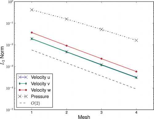
To assert that the present numerical scheme solves the equations correctly, a numerical verification is performed using the method of manufactured solutions (see Roy, 2005) for the solution of the Navier–Stokes equations for an incompressible fluid. The manufactured solution used is presented in the equations below. Four meshes differing only in the refinement adopted per level are used for a mesh convergence test. They are presented numbered as: Mesh 1, 16 × 16 × 16L₂; Mesh 2, 32 × 32 × 32L₂; Mesh 3, 64 × 64 × 64L₂; and Mesh 4, 128 × 128 × 128L₂. Simulations were carried with C_CFL = 0.5 for a total time of 0.1 s. The L₂ norm of the error is calculated and presented in Figure 5, where a second-order decay of errors can be seen, as predicted by the numerical scheme.

Figure 4. Definition of x* and z* variables on the reed's surface.

Figure 5. Mesh convergence test for the code used in the present work.

The equations are as follows: (15) (16) (17) (18) (19) (20)

5. Numerical validation

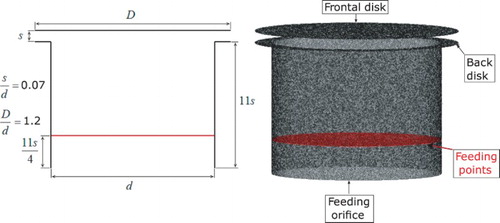
The numerical method used in the present work was validated with experimental results for the incompressible flow through a concentric radial diffuser (Figure 6). The diffuser's geometry was chosen due to its extensive use as a simplified model for reed-type valves (Colaciti et al., 2007; Ferreira et al., 1989; Mariani et al., 2010; Possamai et al., 2001; Prata et al., 1995). Despite its simplicity, the flow through a radial diffuser presents fluid-dynamics phenomena that also occur in the flow through actual valve systems, such as high pressure and velocity gradients, adverse pressure gradients, flow detachment, flow reattachment, and recirculation zones. These phenomena are very difficult to accurately capture in a numerical solution.

Figure 6. Radial diffuser geometric proportions used for the numerical validation.

In order to validate the numerical methodology, the pressure profile along the radial coordinate acting on the frontal disk was compared with the experimental results obtained by using the same experimental bench described by Gasche, Arantes, and Andreotti (2015).

The operational conditions for the validation procedure were D/d = 1.2, s/d = 0.07, and the Reynolds = 2500. Figure 7 shows the domain used to solve the problem and Figure 8 shows the strategy used for the mesh construction, which consists of a mesh of 8 × 8 × 8L9. A total of 9,456,875 Eulerian volumes were used at the beginning of the simulation and the immersed bodies were defined by a Lagrangian mesh of 225,876 Lagrangian points. The Neumann boundary condition with zero derivative was used for all boundaries. The Reynolds number was prescribed at the inlet of the radial diffuser by using the same procedure adopted to define the boundaries of the immersed body, that is, a density force field was prescribed to give a desired velocity (Reynolds number) at the inlet of the geometry.

Figure 7. Calculation domain to solve the flow through a radial diffuser for the numerical validation.

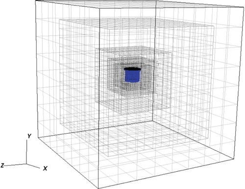
Figure 8. Mesh construction over the diffuser's geometry.

The simulations were carried out for 2, 3, 6, and 12 cycles in the multi-direct forcing procedure. The no-slip boundary condition at the surface of the immersed boundaries was verified through an L₂ norm applied to the velocity field, defined as (21)

As expected, the results show that the L₂ norm decreases for increasing number of cycles. For the same number of cycles, the L₂ norm depends on the position of the body in relation to the flow, because the definition of the no-slip condition at the boundaries depends on the interaction of the fluid with the boundaries. For the frontal disk (Figure 9) and the surface where the Reynolds number is imposed at the feeding orifice (Figure 10), the L₂ norm is of the order of 10⁻² for 2 and 3 cycles, and 10⁻³ for 6 and 12 cycles. However, for the surfaces defining the anterior disk and feeding orifice (Figure 11), the L₂ norm is of the order of 10⁻² for any number of cycles.

Figure 9. Norm evolution with time for different cycling numbers for frontal disk points.

Figure 10. Norm evolution with time for different cycling numbers for feeding points.

Figure 11. Norm evolution with time for different cycling numbers for valve seat points.

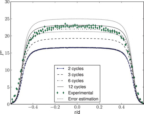
Figure 12 shows the comparison of the results. The dimensionless pressure profiles are plotted as functions of a dimensionless radius (r = d) measured from the center of the frontal disk and presented as a pressure distribution at the central region of the frontal disk due to the stagnation of the flow. As the fluid enters the radial-diffuser region, there is a high-pressure gradient due to the acceleration of the fluid. One can notice that the numerical results get closer to the experimental data for major numbers of cycles. For a number of cycles equal to 12, an error estimation is calculated by performing a Richardson extrapolation of the results obtained with two of the finest refinement levels. Considering an experimental uncertainty of 10%, as in Anhê (2010), one can consider the numerical procedure as validated.

Figure 12. Comparison of pressure profiles obtained in the present simulations with experimental data.

6. New valve-model analysis

This section presents the construction of a new tridimensional model for the representation of the flow through a reed-type valve system. Movement is imposed on the reed to simulate the opening and closing movements. A sinusoidal function is used to calculate the position of each Lagrangian point as a function of time for a given angular frequency and angle displacement range. The entrance flow condition is guaranteed by Lagrangian points placed on the cross-section of the feeding orifice, in which the forces necessary for maintaining this condition are calculated and distributed to the adjacent Eulerian cells. The Eulerian domain is composed by a cube with refinement blocks in the region of the valve model. Reynolds numbers of 1000, 2000 and 3000 are simulated.

The no-slip and entrance flow conditions are verified with L₂ norm calculations for the Lagrangian points and presented on a separated section. A qualitative analysis of the flow is presented, and ring-shaped vortexes are identified. Pressure profiles are also analyzed for the opening and closing movements, and comparisons for different Reynolds numbers are given.

7. Lagrangian domain for the valve

The Lagrangian domain for simulating the flow through the valve is composed by interconnected triangles that form a surface describing the valve model (Figure 1). In the code, the GNU Triangulated Surface (GTS) library is used to deal with the triangulated structure, and a software of free distribution (Geuzaine & Remacle, 2009) is used for generating the geometry and triangulated mesh. An adequate representation of an immersed body is guaranteed if the immersed boundaries of the body are well defined by the finest level of refinement during the simulation. The coupling between the Eulerian and Lagrangian meshes is made through the steps shown in Equations (4(4) ) to (7(7) ). 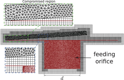Note that the Lagrangian density force must be multiplied by a Lagrangian volume on the distribution process (Equation (6(6) )), which must be properly defined. For this process, each Lagrangian volume is defined as the same size as the Eulerian volume of the finest level. This consideration is reasonable, since the relation presented in Figure 1 is guaranteed at the beginning of the simulations. This relation states that for a simulation to be acceptable, the product of the mean area of all triangular elements with the mean edge of triangles should have an approximately unitary relation with the Eulerian volume of the finest level. Each Lagrangian point is considered to be in the triangle geometric center associated to a triangle face area (Figure 1).

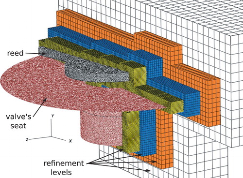
In order to simulate the opening and closing movements of the valve, the angular displacement represented by Equation (22(22) ) is prescribed for the reed model. Due to the requirement of the distribution/interpolation function (Equation (3(3) )), it is necessary to prescribe a minimum angle of inclination of 3.75 in such a way that at least two cells exist between the reed and the seat over the entrance of the flow. This minimum angle is determined considering this stencil in order to not compromise the Lagrangian density force for points close to the feeding orifice. It should be pointed out that it is not possible to avoid the proximity of Lagrangian points between the reed and the valve seat model given the current geometry of the model. Figure 13 shows a side view of the Lagrangian mesh covered by the Eulerian mesh. For the Lagrangian model there is a total of 78,174 points for the boundary force calculations: (22)

Figure 13. Minimum reed inclination angle view with regions affected.

8. Eulerian domain for the valve

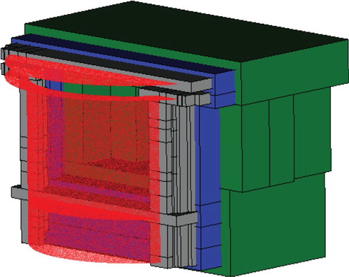
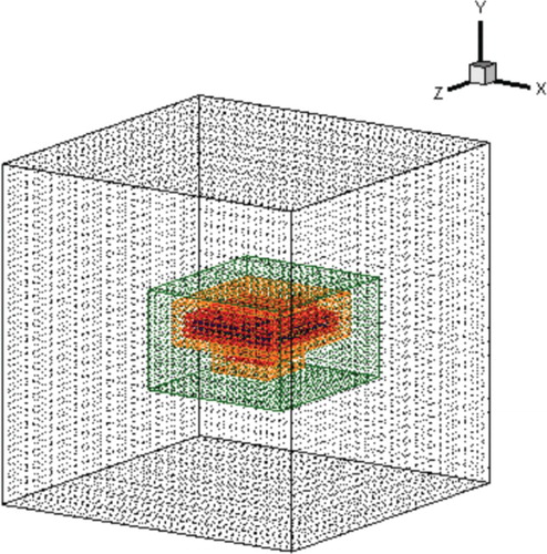
A 12d cubic geometry is used for representing the flow domain (Figure 14). The valve model is placed at the center of the cube, while the refined areas cover the complete Lagrangian domain and guarantee that each Lagrangian point remains at the finest level of refinement. As an SAMR mesh, the grid used can be classified as 24 × 24 × 24L6, as the base level (coarsest) has 24 cells for each direction, and there are 6 refinement levels, including the base level. The finest level covers the immersed boundary with a displacement of Δx = Δy = Δz = 0.03125d. As implemented in the code, Lagrangian and Eulerian volumes must have a unitary ratio. This is the main dependence between both domains, and this restriction imposes a refinement extension across the whole Lagrangian domain.

Figure 14. Eulerian domain with refinement blocks covering the immersed boundary.

Simulations were carried out with Neumann boundary conditions (zero velocity gradients) for all boundaries, except for the north face, for which a Drichlet boundary (no-slip) condition was used. These boundary conditions were chosen for the better convergence achieved when compared with a case set with Neumann boundary conditions for all boundaries. Despite this, the domain size is large compared to the immersed boundary dimensions, which minimizes the effects of the boundary conditions. The integration of the convective terms was accomplished by using the central differencing scheme. The Smagorinsky sub-grid model was used to model the turbulence phenomenon, while the SBDF interpolation scheme was chosen for time integration. A CFL of 0.2 was used in all cases.

9. Results

This section presents the results obtained for the valve model developed in this work. The adequate representation of the rigid body is verified through the evaluation of L₂ norms for each part of the model. Also, the velocity and pressure fields are analyzed. Pressure profiles on the reed's surface are obtained for a better analysis of the flow phenomena.

9.1. Representation of the immersed bodies

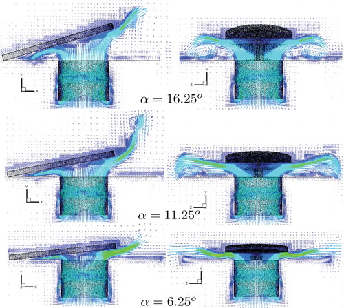
The L₂ norm is the key parameter used to evaluate the quality of the representation of the immersed bodies as it measures the deviation between the velocity at each Lagrangian point used to represent the body and the velocity of the fluid at the same point – that is, it measures the quality of the no-slip condition on the surface of the body. The lower this deviation (L₂ norm) is, the better the representation of the body. Figure 15 shows the behavior of the L₂ norm at the reed points for Re = 1000; it can be seen that the L₂ norm varies with the angular velocity of the reed. Its maximum value was about 0.085 for α = 11.25°, which is the position of the maximum reed velocity, while the minimum values of about 0.01 and 0.005 were obtained for α = 3.75° and α = 18.25°, respectively, where the reed velocity is zero. The L₂ norm also varies with the Reynolds number. For Re = 3000, an increase in the L₂ norm is observed of 5% for α = 18.25° and 13% for α = 3.75°. These increases are due to the increase of the velocity gradients near the surface defining the body for increasing Reynolds numbers.

Figure 15. L2 norm evolution with time for the model presented in this work.

Figure 15 shows the L₂ norm for the boundaries representing the seat for Re = 1000, where it can be seen that it stabilizes rapidly to a value of the order of 0.02. In addition, this value was not significantly affected by the Reynolds number. The same behavior of the L₂ norm was obtained for the boundary used to prescribe the velocity of the fluid at the feeding orifice. In this case, the L₂ norm stabilized to a value of the order of 0.06 (Figure 15).

As can be seen in the velocity fields in Figures 16 to 19, L₂ norms of the order of 10⁻² proved to be sufficient to provide the no-slip condition at the surfaces of all immersed boundaries.

Figure 16. Vector field on a slice passing through the center of the feeding orifice for the opening movement.

9.2. Velocity vector field

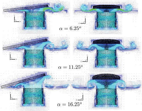
In order to evaluate the adequacy of the numerical methodology one can also observe the behavior of the velocity and pressure fields of the flow. Figures 16 and 17 show the magnitude of the velocity vector field for Re = 1000 during the opening and closing of the reed, respectively. First of all, the L₂ norm of the order of 10⁻² seems to be sufficient for identifying the immersed bodies, which can be qualitatively confirmed through the deviations of the flow produced by the solid surfaces. Second, the dynamics of the flow is completely different depending on whether the reed is opening or closing. For the opening movement of the reed, there are recirculating bubbles produced by the right exit corner of the feeding orifice. The inertial forces of the flow are sufficient to produce the detachment of the flow at this position, causing the formation of the recirculating bubble. As expected, the intensity of the recirculating bubble decreases for increasing angles because of the reduction of the local velocities. For larger angles one can notice the formation of a second recirculating bubble near the position where the reed is installed, which is caused by the left exit corner of the feeding orifice. The reason for this is the increase in the height of the channel formed between the reed and the seat, which reduces the viscous forces in comparison with the inertial forces of the flow. In addition, it is also possible to observe that the flow is symmetrical in relation to the y-axis. In Figure 17, it can be seen that the recirculating bubbles are suppressed by the closing movement of the reed, mainly for the lower angles.

Figure 17. Vector field on a slice passing through the center of the feeding orifice for the closing movement.

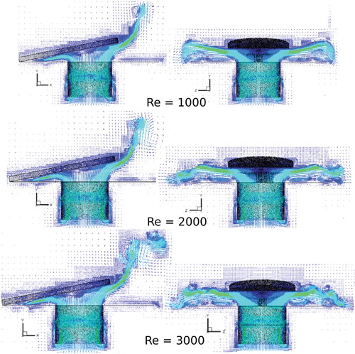
The influence of the Reynolds number on the opening and closing movement of the reed can be seen in Figures 18 and 19, respectively, where the velocity vector field is plotted for Re = 1000, Re = 2000, and Re = 3000. For the opening movement (Figure 18), the general patterns of the flow are very similar, but it is possible to see through the color grade that the intensity of the velocity vectors increases for increasing Reynolds numbers, mainly for the two eddies formed at the exit of the right-hand side of the reed. In the case of the closing movement (Figure 19), the differences in the flow patterns are more evident. The number and intensity of the eddies increase for increasing Reynolds numbers, which is consistent with the turbulence phenomenon.

Figure 18. Vector field on a slice passing through the center of the feeding orifice for the opening movement for different Reynolds numbers.

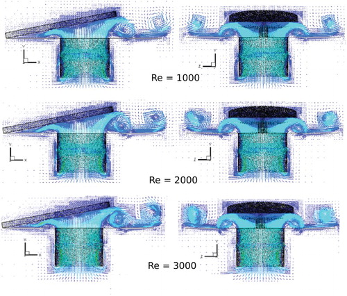
Figure 19. Vector field on a slice passing through the center of the feeding orifice for the closing movement for different Reynolds numbers.

9.3. Pressure field

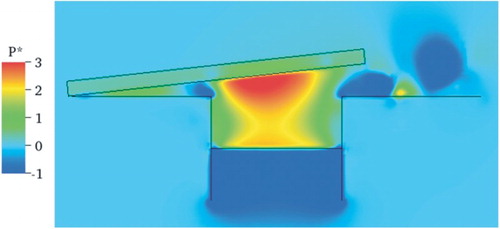
Analyzing the pressure field is another way to evaluate the numerical methodology. Figures 20 to 22 present the pressure field at a z plane passing through the center of the geometry for α = 6.25° and Re = 1000 to 3000. In all cases there is a high-pressure region approximately at the center of the circular part of the reed which is coincident with the stagnation region of the flow depicted in Figures 16 and 17. This behavior was expected due to the conversion of the kinetic energy to pressure energy as the flow hits the reed. In addition, the eddies in the velocity vector field are coincident with the low-pressure regions, which is a result corroborated by the turbulence theory.

Figure 20. Pressure field at a z plane passing through the center of geometry for α = 6.25° and Re = 1000.

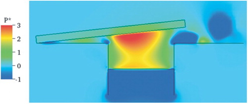
Figure 21. Pressure field at a z plane passing through the center of geometry for α = 6.25° and Re = 2000.

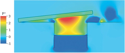
Figure 22. Pressure field at a z plane passing through the center of geometry for α = 6.25° and Re = 3000.

9.4. Pressure profile

Dimensionless pressure profiles on the reed surface are plotted in Figures 23to 26 using the coordinate system indicated in Figure 4. Figure 23 shows pressure profiles in the x*-axis for Re = 1000 and different aperture angles. It is possible to observe similar patterns in the pressure profiles for several aperture angles. The center of the circular region of the reed (1.0 < x* < 2.3) is where the larger pressures occur, and it decreases as the flow goes to the diffuser region (between reed and seat) as the passage is restricted by the proximity of the reed and seat. For 0.5 < x* < 1.0 the pressure increases while the velocity field decreases its magnitude downstream of a whirl formed as the flow accelerates in the diffuser's entrance. After this, the pressure rises again due to friction forces.

Figure 23. Pressure profiles in x* for the opening movement.

With angle augmentation up to α = 11.25° there is a pressure decrease due to the diminishing of the friction forces acting on the reed as it accelerates. After this, the pressure starts to increase again with the deceleration of the reed until α = 16.25°. The same behavior is observed in Figure 24, in which similar pressure profiles are plotted in the z direction. The pressure profiles confirm the symmetry of the flow observed in the velocity vector field.

Figure 24. Pressure profiles in z* for the opening movement.

For the closing movement of the reed, the general characteristics of the pressure profiles are similar (Figures 25 and 26). However, it is evident that the pressure levels are larger due to the augmentation of the relative velocity of the flow in relation to the reed. In addition, the pressure variations are much lower owing to the suppression of the eddies.

Figure 25. Pressure profiles in x* for the closing movement.

Figure 26. Pressure profiles in z* for the closing movement.

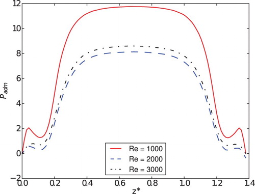
The influence of the Reynolds number on the pressure distribution on the reed surface is analyzed in Figures 27to 30. Figure 27 shows the pressure profile in the x direction for α = 6.25° during the opening movement of the reed and the patterns of the pressure profiles are similar for all Reynolds numbers. However, the acceleration of the flow for Re = 3000 and x* < 1.0 is higher, producing larger oscillations. The pressure profiles in the z* direction are almost independent of the Reynolds number. The same results are presented for the closing movement and the same angle in Figure 29. First of all, the pressure levels are much higher in this case because the relative velocities are higher during the closing movement. Second, the pressure oscillations for x* < 1.0 are much lower in this case due to the suppression of the recirculation formation caused by the closing movement. Comparing Figures 16 and 17, it can be seen that the recirculation is greater during the opening movement and the pressure level for Re = 1000 is higher because the dimensionless pressure is obtained by dividing the pressure by the square average velocity of the flow.

Figure 27. Pressure profiles in x* for the opening movement for different Reynolds numbers and α = 6.25°.

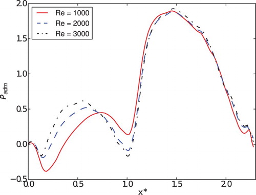
Figure 28. Pressure profiles in z* for the opening movement for different Reynolds numbers and α = 6.25°.

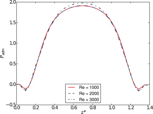
Figure 29. Pressure profiles in x* for the closing movement for different Reynolds numbers and α = 3.75°.

Figure 30. Pressure profiles in z* for the closing movement for different Reynolds numbers and α = 3.75°.

10. Conclusion

A new numerical methodology for solving the fluid structure interaction problem present in the flow through reed-type valves has been reported in this paper. A geometry usually used in suction valves of refrigeration compressors has been used for modeling the reed. The numerical methodology has been described in detail and the numerical results are experimentally validated through the pressure distribution acting on the frontal disk of a radial diffuser. The numerical results for the velocity and pressure fields for Reynolds numbers based on the inlet conditions of the flow of 1000, 2000, and 3000 were comprehensively explored during the opening and closing movements of the reed. The results of the study show that the numerical methodology presented here is very promising with regard to solving the flow in the actual dynamics of reed-type valves.

Acknowledgements

This research developed at the Universidade Estadual Paulista ‘Júlio de Mesquita Filho’.

Disclosure statement

No potential conflict of interest was reported by the authors.

ORCID

José Luiz Gasche http://orcid.org/0000-0002-3652-8216

Aristeu da Silveira Neto http://orcid.org/0000-0002-1392-3758

Millena Martins Villar http://orcid.org/0000-0002-2084-8602

Additional information

Funding

This work was supported Higher Education Personnel Improvement Coordination (CAPES), Tecumseh of Brazil and Petrobras.

References

- Alvarez, C. M. R. (2013). Simulação computacional adaptativa de escoamentos bifásicos viscoelásticos [Adaptive computational simulation of biphasic viscoelastic flows] (Doctoral dissertation). Retrieved from http://www.teses.usp.br/teses/disponiveis/45/45132/tde-07082013-112937/pt-br.php
- Anhê Jr., S. A. (2010). Investigação numérica e experimental do escoamento em válvulas de compressores herméticos [Numerical and experimental investigation of the flow in hermetic compressor valves] (Master's. thesis). Retrieved from http://repositorio.unesp.br/bitstream/handle/11449/88864/anhejunior_sa_me_ilha.pdf?sequence=1
- Ascher, U. M., Ruuth, S. J., & Wetton, B. T. R. (1995). Implicit-explicit methods for time-dependent partial differential equations. SIAM Journal on Numerical Analysis, 32(3), 797–823. doi:10.1137/0732037
- Chorin, A. J. (1968). Numerical solution of the Navier-Stokes equations. Mathematics of Computation, 22(104), 745–762. Retrieved from https://math.berkeley.edu/~chorin/chorin68.pdf doi: 10.1090/S0025-5718-1968-0242392-2
- Colaciti, A. K., López, L. M. V., Navarro, H. A., & Cabezas-Gmez, L. (2007). Numerical simulation of a radial diffuser turbulent airflow. Applied Mathematics and Computation, 189(2), 1491–1504. doi:10.1016/j.amc.2006.12.029
- Courant, R., Friedrichs, K., & Lewy, H. (1967). On the partial difference equations of mathematical physics. IBM journal of Research and Development, 11(2), 215–234. doi:10.1147/rd.112.0215
- Ferreira, R. T. S., Deschamps, C. J., & Prata, A. T. (1989). Pressure distribution along valve reeds of hermetic compressors. Experimental Thermal and Fluid Science, 2(2), 201–207. doi:10.1016/0894-1777(89)90034-4
- Ferziger, J. H. & Peric, M. (1996). Computational methods for fluid dynamics. Berlin: Springer.
- Gasche, J. L., Arantes, D. M. & Andreotti, T. (2015). Pressure distribution on the frontal disk for turbulent flows in a radial diffuser. Experimental Thermal and Fluid Science, 60, 317–327. doi:10.1016/j.expthermflusci.2014.10.005
- Geuzaine, C., & Remacle, J. F. (2009). Gmsh: a three-dimensional finite element mesh generator with built-in pre- and post-processing facilities. International Journal for Numerical Methods in Engineering 79(11), 1309–1331. doi: 10.1002/nme.2579
- Kim, H., Ahn, J., & Kim, D. (2008). Fluid structure interaction and impact analyses of reciprocating compressor discharge valve. In International Compressor Engineering Conference at Purdue: Vol 1210, West Lafayette. Retrieved from http://docs.lib.purdue.edu/cgi/viewcontent.cgi?article=2935&context=icec
- Kinjo, K., Nakano, A., Hikichi, T., & Morinishi, K. (2010). Study of CFD considering valve behavior in reciprocating compressor. In International Compressor Engineering Conference at Purdue, West Lafayette. Retrieved from http://docs.lib.purdue.edu/cgi/viewcontent.cgi?article=2974&context=icec
- Lima, R. S. (2012). Desenvolvimento e implementação de malhas adaptativas bloco-estruturadas para computação paralela em mecânica dos fluidos [Development and implementation of a parallelization methodology for adaptive block structured meshes] (Doctoral dissertation). http://hdl.handle.net/123456789/3911
- Machu, G., Albrecht, M., Bielmeier, O., Daxner, T., & Steinruck, P. (2004). A universal simulation tool for reed valve dynamics. In International Compressor Engineering Conference at Purdue, West Lafayette. Retrieved from http://docs.lib.purdue.edu/cgi/viewcontent.cgi?article=2715&context=icec
- Mariani, V. C., Prata, A. T., & Deschamps, C. J. (2010). Numerical analysis of fluid flow through radial diffusers in the presence of a chamfer in the feeding orifice with a mixed Eulerian-Lagrangian method. Computers and Fluids, 39(9), 1672–1684. doi:10.1016/j.compfluid.2010.06.003
- Mistry, H., Bhakta, A., Dhar, S., Bahadur, V., & Dey, S. (2012). Capturing valve dynamics in reciprocating compressors through computational fluid dynamics. In International Compressor Engineering Conference at Purdue, volume 1210, West Lafayette.
- Mittal, R. & Iaccarino, G. (2005). Immersed boundary methods. Annual Review of Fluid Mechanics, 37, 239–261. doi:10.1146/annurev.fluid.37.061903.175743
- Nós, R. L. (2007). Simulações de escoamentos tridimensionais bifásicos empregando métodos adaptativos e modelos de campos de fase [Simulations of tridimensional flows using adaptive methods and phase field models] (Doctoral dissertation). Retrieved from http://www.teses.usp.br/teses/disponiveis/45/45132/tde-08052007-143200/en.php
- Pereira, E. L., Santos, C. J., Deschamps, C. J., & Kremer, R. (2012). A Simplified CFD Model for Simulation of the Suction Process of Reciprocating Compressors. In International Compressor Engineering Conference at Purdue, volume 1276, West Lafayette. Retrieved from http://docs.lib.purdue.edu/icec/2086/
- Peskin, C. S. (1973). Flow patterns around heart valves. In Proceedings of the Third International Conference on Numerical Methods in Fluid Mechanics (pp. 214–221). Springer Berlin Heidelberg. Retrieved from http://link.springer.com/chapter/10.1007/BFb0112697#
- Possamai, F., Ferreira, R., & Prata, A. (2001). Pressure distribution in laminar radial flow through inclined disks. International Journal of Heat and Fluid Flow, 22(4), 440–449. doi:10.1016/S0142-727X(01)00109-6
- Prata, A. T., Pilichi, C. D. M., & Ferreira, R. T. S. (1995). Local heat transfer in axially feeding radial flow between parallel disks. Journal of heat transfer, 117(1), 47–53. doi:10.1115/1.2822321
- Ribas, J. F. A., Deschamps, C. J., Fagotti, F., Morriesen, A., & Dutra, T. (2008). Thermal analysis of reciprocating compressors – a critical review. In International Compressor Engineering Conference at Purdue, West Lafayette. Retrieved from http://docs.lib.purdue.edu/cgi/viewcontent.cgi?article=2906&context=icec
- Roy, C. J. (2005). Review of Code and Solution Verification Procedures for Computational Simulations. Journal of Computational Physics, 205(1), 131–156. doi: 10.1016/j.jcp.2004.10.036
- Smagorinsky, J. (1963). General circulation experiments with the primitive equations: I. the basic experiment. Monthly weather review, 91(3), 99–164. doi: 10.1175/1520-0493(1963)091<0099:GCEWTP>2.3.CO;2
- Villar, M. M. (2007). Análise numérica detalhada de escoamentos multifásicos bidimensionais [Detailed numerical analysis of multiphasic bidimensional flows] (Doctoral dissertation). doi: http://hdl.handle.net/123456789/120
- Wang, Z., Fan, J., & Luo, K. (2008). Combined multi-direct forcing and immersed boundary method for simulating flows with moving particles. International Journal of Multiphase Flow, 34(3), 283–302. doi:10.1016/j.ijmultiphaseflow.2007.10.004 doi: 10.1016/j.ijmultiphaseflow.2007.10.004