
ABSTRACT
Transitions are structures that can change geometry and flow velocity through varying the cross-sections of their channels. Under subcritical flow and steady flow conditions, it is necessary to reduce the flow velocity gradually due to increasing water pressure and adverse pressure gradients. Due to the separation of flow and subsequent eddy formation, a significant energy loss is incurred along the transition. This study presents the results of experimental investigations of the subcritical flow along the expansive transition of rectangular to trapezoidal channels. A numerical simulation was developed using a finite volume of fluid (VOF) method with a Reynolds stress turbulence model. Water surface profiles and velocity distributions of flow through the transition were measured experimentally and compared with the numerical results. A good agreement between the experimental and numerical model results showed that the Reynolds model and VOF method are capable of simulating the hydraulic flow in open channel transitions. Also, the efficiency of the transition and coefficient of energy head loss were calculated. The results show that with an increasing upstream Froude number, the efficiency of the transition and coefficient of energy head loss decrease and increase, respectively. The results also show the ability of numerical simulation to simulate the flow separation zones and secondary current along the transition for different inlet discharges.
Nomenclature
| The following symbols are used in this paper: | ||
| ui | = | mean velocity in the xi-direction |
| uj | = | mean velocity in the yj-direction |
| k | = | turbulence kinetic energy |
| u0 | = | average inlet velocity |
| L | = | transition length |
| b0 | = | bed width of rectangular channel |
| b | = | bed width of transition |
| bL | = | bed width of trapezoidal channel |
| m | = | side slope of transition |
| mL | = | side slope of trapezoidal channel |
| V1 | = | average velocity at section 1 |
| V2 | = | average velocity at section 2 |
| ke | = | energy loss coefficient |
| Hi | = | total energy head |
| g | = | gravity acceleration |
| ρ | = | fluid density |
| y1 | = | depth of flow at section 1 |
| y2 | = | depth of flow at section 2 |
| α1 | = | energy correction factor at transition inlet |
| α2 | = | energy correction factor at transition outlet |
| z | = | measured point height |
| ϵ' | = | turbulence dissipation rate |
| ϵ | = | efficiency |
| ν | = | molecular viscosity |
| νt | = | turbulent viscosity |
| Fr1 | = | inflow Froude number |
| Q | = | inlet discharge |
1. Introduction
Open channel transitions are small hydraulic structures used for changing the cross-sectional area and flow pattern (Henderson, Citation1966). A more complicated case is the combination of the above-mentioned geometric features. Channel expansions are commonly encountered in both natural open channels and constructed hydraulics facilities, such as the flow through subdivided channels between bridge piers and the water flowing out of culverts. In the case of a flow diversion channel for hydropower generation, which often incorporates one or more expansions, the losses of flow energy in the expansions will mean less electrical power generated at the downstream hydropower plant (Najafi-Nejad-Nasser, Citation2011). In the case of irrigation channels with expansions, the losses of flow energy in the expansions reduces the efficiency of the irrigation systems. The issue of flow energy losses in channel expansions is relevant and important in many other hydraulics engineering applications (Najafi-Nejad-Nasser, Citation2011). With a decreasing flow depth and increasing Froude number, the dimensions of the flow separation zones increase, as do the energy losses along the transition. Abbott and Kline (Citation1962) observed asymmetric flow patterns on an expansion transition in their experimental investigations. They also found that the Reynolds numbers and turbulence intensities have no effect on flow pattern. Ramamurthy et al. (Citation1970) studied separation zones in a gradual transition and the suppression of flow separation by fitting a simple hump at the channel bottom, experimentally. They showed that both the angle of divergence and the length of transition relative to the inlet dimension have an effect on flow separation. Nashta and Grade (Citation1988) present the results of analytical and experimental investigations of channels with a sudden expansion for subcritical flow. Swamee and Basak (Citation1992) discuss a method for the design of expansions that connect a rectangular channel section with a trapezoidal channel section for subcritical flow. They suggest that flow separation in the expansion and the associated energy losses were considerably reduced. Manica and Bortoli (Citation2003) consider laminar flow with a low Reynolds number in a symmetric sudden expansion, numerically. Their results show that below a certain critical Reynolds number (about 50) the flow pattern is symmetric around the channel central line. Hsu, Su, and Chang (Citation2004) suggest a method for estimating the optimal length of the contraction transition under supercritical flow using the ratio of downstream to upstream channel width. They conclude that as the ratio of constriction increases the optimal length of the contraction transition decreases. Alauddin and Basak (Citation2006) examined the flow hydraulic in an abrupt expansion, experimentally. The purpose of their study was to design an expanding transition with minimum flow separation and hence small energy head losses. Velocity distributions of flow through the sudden as well as gradual expansion models were made, thus, a transition profile for the expansion of flow with minimum separation was evolved by streamlining the boundary shape of the transition. Haque (Citation2008) investigated flow velocity profiles, turbulence kinetic energy and turbulence intensity in expansive transitions, along with the effect of the hump location on bed shear stress. Basak and Alauddin (Citation2010) studied the effect of different upstream Froude numbers and inlet discharges on the efficiency of the transition in an expansive transition. They show that as the upstream Froude number and inlet discharge increase, the efficiency of the transition decreases. As numerical hydraulic models can significantly reduce the costs associated with experimental models, their use has been rapidly expanded in recent decades. Some methods use finite elements (Chau & Jiang, Citation2001, Citation2004; Wu & Chau, Citation2006) and others use finite volume in numerical modeling (Epely-Chauvin, De Cesare, & Schwindt, Citation2014; Gholami, Akhtari, Minatour, Bonakdari, & Javadi, Citation2014; Liu and Yang, Citation2014). Howes, Burt, and Sanders (Citation2010) studied flow velocity profiles along the contraction transition for different inlet Froude numbers and inlet positions under subcritical flow, experimentally. Najafi-Nejad-Nasser and Li (Citation2014) investigated the effectiveness of fitting a hump at the expansion's bottom with the aim of reducing flow separation and energy loss. They report on analytical solutions to the problem of flow transition and associated energy head loss by using the concepts of momentum and energy. This study presents an experimental and numerical investigation of the flow field in the gradual transition of rectangular to trapezoidal open channels. A numerical simulation was developed using the finite-volume method with a Reynolds stress turbulence model. After calibration, the created secondary currents and effect of the different inlet discharges on the created separation zones at the transition corners were investigated.
2. Design method
Because of the importance of knowledge concerning expansions in rigid-bed channels, several investigators have studied the different aspects of flow in expansion. In this study, for the design of the expansion transitions of rectangular to trapezoidal channels, the method of Swamee and Basak (Citation1992) is used, which is briefly outlined here (Figure ).
Figure 1. Definition sketch: expansive transition of rectangular to trapezoidal.
The bed-width profile is given in the following equation (Swamee & Basak, Citation1992):
(1)
where a, p, and q are unknown positive numbers called transition parameters and ζ = x/L, where L is the transition length and x is distance from the transition inlet . The transition parameters are obtained by:
(2)
where N is the total number of bed-width profiles and E(a,p,q) is minimized by a grid-search algorithm. The optimal bed-width profile is obtained by (Swamee & Basak, Citation1992):
(3)
which can be written as:
(4)
where b0, b, and bL are the bed width of the rectangular channel, the bed width of the transition, and the bed width of the trapezoidal channel, respectively. Analyzing a large number of optimal side-slope profiles, an equation was presented as:
(5)
where m and mL are the side slope of the transition and the side slope of the trapezoidal channel, respectively. Equation (5) can be simplified as (Swamee & Basak, Citation1992):
(6)
3. Experimental setup
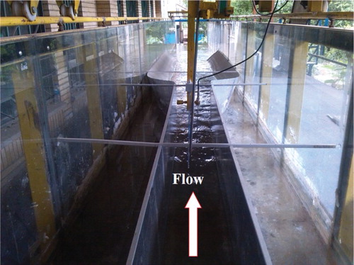
The experiments were performed in a flume of 11 m length, 1 m width and 0.8 m height, which consisted of a steel frame and bed, and side walls of glass sheet. A transition of 1 m length was connected to an upstream rectangular channel of 3 m length and 0.25 m and a downstream trapezoidal reach with a bed width of 0.4 m and a side slope ratio of 1:1.
Flow discharge was measured using a flow meter located in the supply pipe. Water was supplied from a sump into the entrance tank. The water level was measured with a point-gauge instrument with a measurement accuracy of 0.01 mm. The rails were provided along the entire working length of the flume, which supports a moving carriage. The velocity was also measured with a micro Moline instrument with a measurement accuracy of 0.001 m/s (Figure ).
Figure 2. Experimental setup for flow depth and velocity measurements.
To obtain the velocity distribution of flow through expansion and hence evaluate the efficiency of the transition, the velocity and flow depth were measured at different points. Velocities were measured near the water surface, 0.20y, 0.40y, 0.60y, 0.80y and near the bottom in the vertical. These measurements were made at a number of sections across the transition reach at 1/8, 3/8, 1/2, 5/8 and 7/8 times the width (Figure ) and along the length of transition at the inlet, middle and outlet sections. The experiments were conducted with five different discharges of 10, 15, 20, 25 and 30 l/s. Table shows range of flow hydraulic characteristics.
Figure 3. (a) Top view of flume and (b) a section showing the points where velocity measurements were taken.
Table 1. Range of flow hydraulic characteristics.
4. Efficiency and coefficient of the energy head loss
For finding the efficiency, it is necessary to consider the velocity variation across the channel. Assuming that the flow is essentially in the direction of the axis of the transition, the efficiency of the transition is defined by (Basak & Alauddin, Citation2010):
(7)
where Q is the inlet discharge, g is the gravity acceleration, ρ is the fluid density, y1 and y2 are the depth of flow at sections 1 and 2, respectively, α1 and α2 are the energy correction factors at the inlet and outlet sections of the transition, respectively, and V1 and V2 are the average velocities at sections 1 and 2, respectively.
Using the data for flow depth and local velocity, the flow area and average velocity at the sections were known – thus the energy correction factors could be calculated. These data were used to evaluate the efficiency of the transition. The energy loss coefficient is defined as (Najafi-Nejad-Nasser, Citation2011):
(8)
where ke is the energy loss coefficient and Hi is the total energy head equal to the sum of the velocity head, elevation head and pressure head.
5. Mathematical modeling
5.1. Governing equations
In this study, a finite-volume method with a Reynolds stress turbulence model was developed. The continuity and momentum equations for incompressible turbulent flow in a 3D form are defined below (Haque, Citation2008), along with the turbulence kinetic energy:
(9)
(10)
where τij is the stress tensor and for turbulent flow is defined as:
(11)
(12)
where Ui and Uj are the mean velocities in the xi and yi directions, respectively, 't is the time, P is the pressure,
is the Reynolds stress, gxi is the acceleration due to gravity, and k is the turbulence kinetic energy (Olsen, Citation2008). Quick and second-order upwind schemes were used for solving momentum and turbulence equations, respectively. A standard method was used for the discretization of the pressure equation. The transport equation in the Reynolds stress turbulence model is:
(13)
where Pij is the production tensor, and Φij and
are the strain pressure and dissipation tensors, respectively (Versteeg & Malalasekera, Citation2007). In this study, for simulating the free surface, a volume of fluid (VOF) method is used as follows:
(14)
where
is the fraction of water. In this paper, the free surface is defined by
= 0.5, which is a common value for this purpose in the literature.
5.2. Boundary conditions
In the 3D simulations performed in the present study, the boundaries depending on the nature of the flow were solid walls, inlet, outlet and free surface. The water velocity was defined at the inlet section with a known water depth entering the flow domain and inlet discharge and the air velocity at the flow inlet was applied at 1e−5 m/s. k and were obtained as follows (Versteeg & Malalasekera, Citation2007):
(15)
(16)
where
is the average inlet velocity,
is the turbulence intensity that is typically between 1% and 5% and depends on the upstream flow,
is constant and equal to 0.09, and L' is 0.07 of the hydraulic diameter (Versteeg & Malalasekera, Citation2007). For air-surface modeling, the pressure inlet boundary condition was used. To estimate the wall effects on the flow, empirical wall functions known as standard wall functions were used. The grid structure must be fine enough, especially near the wall boundaries and the expansion, which is the region of rapid variation. The generated mesh is non-uniform. The cells number in the x, y, and z directions are 60 × 15 × 21 in the upstream channel, 30 × 15 × 21 in the expansion and 50 × 15 × 21 in the downstream channel. The utilized mesh shape at this study is rectangular. The distances of the nearest grid to the transition wall and the upstream channel are 0.9 mm and 5 mm, respectively. The minimum mesh dimension in the computational domain is 0.0009 m × 0.033 m and the maximum mesh dimension is 0.0185 m × 0.049 m. Figure shows a plan and 3D view of the generated mesh in the computational domain.
Figure 4. (a) Plan and (b) 3D view of the generated mesh in the computational domain.
6. Experimental observations and results
As mentioned, for finding the efficiency, it is necessary to consider the velocity values and water level along the channels. Figure shows the measured water level along the center line of the channels for different Froude numbers and Q = 10 l/s. The measured velocities near the water surface for Fr1 = 0.47 are presented in Figure .
Figure 5. Measured water surface profiles for different Froude numbers for Q = 10 l/s.
Figure 6. Velocity distributions across the width and along the length of the transition.
As seen in Figure , the flow depth increases along the expansive transition. Fr1 = 0.70 has the maximum water surface slope and Fr1 = 0.32 has the minimum slope. It is shown that as the inlet Froude number increases, the water surface slope also increases. According to Figure , with the exception of Q = 10 l/s the flow is never symmetrical with respect to the centerline of the channel. The maximum velocity line coincides with the center line of the channel for a short length after entry. Thereafter, it shifts to the side to which the main flow is attached. The reason for the deviation between the maximum velocity line and centerline is related to the asymmetrical circulation and secondary flow that occurred in the cross-sections given for x = 3L/5 and x = 4L/5 (as shown later in this section). The maximum velocity line and centerline do not match, due to the flow separation zones and secondary flow created at transition corners. For discharges greater than 10 l/s, velocities at transition corners are negative and close to zero, indicating that flow separation zones are formed there. Also, along the transition, the velocities decrease with approaching the transition outlet. The efficiency of the transition and the energy loss coefficient along the transition are presented in Figures and , respectively.
Figure 7. Efficiency of the transition for different inlet discharges.
Figure 8. Energy loss coefficient along the transition for different Froude numbers.
As shown in Figure , the overall hydraulic efficiency of the transition increases from Q = 30 l/s to Q = 10 l/s, and these are 30.36%, 35.45%, 39.98%, 48.32% and 60.83%. The efficiency for Q = 10 l/s is the highest among the models at 60.83%. As the inlet Froude number increases from Fr1 = 0.47 to Fr1 = 0.70 the efficiency of the transition decreases due to the increasing water surface slope, which also causes the process efficiency to decrease. Also, from Fr1 = 0.32 to Fr1 = 0.47 as the inlet discharge increases the slope down efficiency decreases. As shown in Figure , as the inlet Froude number increases the energy loss coefficient also increases. The maximum value of the energy loss coefficient is equal to 0.609 and occurs at Fr1 = 0.70. Also, as the inlet discharge increases, the energy loss coefficient again increases. Figure compares the simulated water surface profiles with the experimental data along the transition for inlet Froude numbers and Q = 20 l/s.
Figure 9. Water surface profiles for different inlet Froude numbers for Q = 20 l/s.
For error percentage calculation, the root mean square error (RMSE) method was used. The RMSEs obtained for Fr1 = 0.32 to Fr1 = 0.70 are 0.458%, 0.676%, 0.895%, 1.795%, 1.310% and 0.866%. The measured and numerical velocity data in the x direction (ux) along the transition for Q = 10 l/s and Fr1 = 0.47 are presented in Figure . The velocity values are dimensionless by the inlet flow velocity (u0) and z is measured points depth.
Figure 10. Velocity distribution for Q = 10 l/s and Fr1 = 0.47 at (a) the transition inlet, (b) the transition middle and (c) the transition outlet.
As seen in Figure , similar to the measured results, the longitudinal velocity decreases as the transition outlet is approached. The RMSEs obtained at the transition inlet, transition middle and transition outlet are 4.962%, 6.234% and 4.575%, respectively. Consequently, for the evaluation of the flow separation zone in transition, Figure shows the streamline near the water surface for Fr1 = 0.47 and different discharges of 10 l/s, 15 l/s, 20 l/s and 25 l/s.
Figure 11. Streamlines near the water surface for different discharges.
As seen in Figure , as the inlet discharge of the expansion increases, the length and width of the flow separation zone increase as well. Also, as the upstream Froude number increases, so does the energy loss coefficient. Thus it can be concluded that flow separation zones are a reason for increases in energy losses. For Q = 10 l/s to Q = 25 l/s, the lengths of separation zone are obtained as 0.16 m, 0.62 m, 0.67 m and 0.98 m and the widths of the separation zone increase from 0.039 m to 0.25 m. Due to the imbalance lateral pressure gradient and centrifugal force, a spiral flow (secondary current) generates in different cross-sections of the transition, which results in bed sediment transport. Figure shows the secondary currents along the expansion channel for Fr1 = 0.47.
Figure 12. Streamlines in various cross-sections along the transition for Q = 25 l/s.
According to the Figure , two small circulation zones are observed at the transition entrance (x = 0.00). Approaching the middle of the transition, the number of circulation zones increases, as at x = 3L/5 and x = 4L/5, three and four circulation zones are generated, respectively. The number of circulation zones decreases at the outlet section of the transition (x = L). Therefore, at x = 3L/5 and x = 4L/5, the secondary current strength is greater than in the other sections.
7. Conclusions
This study presents the results of experimental investigations of the subcritical flow through the transition in a rectangular to trapezoidal open channel. A flow numerical simulation was performed in the transition and Reynolds-averaged Navier–Stokes (RANS) equations were solved using a finite-volume method. The flow calculations were performed using a Reynolds stress turbulence model. It is suggested that for improvements and the future direction of this work, the effect of the channel-bed roughness, the fitting of a hump to the bed transition and the transition length on the dimensions of the flow separation zones, efficiency and energy loss coefficient along the transition be studied. The findings of the present study are as follows:
The measured flow depth increases along the expansive transition. It is shown that the inlet Froude number is one of the parameters which has an effect on the water surface slope.
As the inlet Froude number increases, the efficiency of the transition decreases. As the water surface slope increases, the process efficiency decreases. Also, as the inlet discharge and Froude number increase, so too does the energy loss coefficient.
The flow pattern along the expansion is asymmetric (except for Q = 10 l/s). The maximum velocity line coincides with the centerline of the channel for a short length after entry. Thereafter, it shifts to the side to which the main flow is attached. The reason for the deviation between the maximum velocity line and centerline is related to the asymmetrical circulation and the secondary flow that occurs in the cross-sections given for x = 3L/5 and x = 4L/5.
For discharges greater than 10 l/s, the velocities at transition corners were negative and close to zero, indicating that flow separation zones form there. A good agreement was found between the numerical simulation of the velocity profiles and the experimental results.
The inlet discharge of expansion has an effect on the flow pattern in the expansion. As the inlet discharge of the expansion increases, the length and width of the flow separation zone increase as well. Also, as the upstream Froude number increases, so too does the energy loss coefficient. Thus, it can be concluded that the flow separation zones are a reason for increases in energy losses.
Approaching the middle of the transition, the number of circulation zones increases and is more than in other sections at x = 3L/5 and x = 4L/5. The number of circulation zones decreases at the outlet section of the transition.
Acknowledgments
Experiments were supported by laboratory of Gorgan University of Agricultural Sciences and Natural Resources, Department of Water Engineering. My completion of this paper could not have been accomplished without the support of this university.
Disclosure statement
No potential conflict of interest was reported by the authors.
References
- Abbott, D. E., & Kline, S. J. (1962). Experimental investigation of subsonic turbulent flow over single and double backward facing steps. Journal of Basic Engineering, 84, 317. doi: 10.1115/1.3657313
- Alauddin, M., & Basak, B. C. (2006). Development of an expansion transition in open channel sub-critical flow. Journal of Civil Engineering, 34(2), 91–101.
- Basak, B. C., & Alauddin, M. (2010). Efficiency of an expansive transition in an open channel subcritical flow. DUET Journal, Dhaka University of Engineering & Technology, 1(1), 27–32.
- Chau, K. W., & Jiang, Y. (2001). 3D numerical model for Pearl river estuary. Journal of Hydraulic Engineering, 127(1), 72–82. doi: 10.1061/(ASCE)0733-9429(2001)127:1(72)
- Chau, K. W., & Jiang, Y. (2004). A three-dimensional pollutant transport model in orthogonal curvilinear and sigma coordinate system for Pearl river estuary. International Journal of Environment and Pollution, 21(2), 188–198. doi: 10.1504/IJEP.2004.004185
- Epely-Chauvin, G., De Cesare, G., & Schwindt, S. (2014). Numerical modelling of plunge pool scour evolution in non-cohesive sediments. Engineering Applications of Computational Fluid Mechanics, 8(4), 477–487. doi: 10.1080/19942060.2014.11083301
- Gholami, A., Akhtari, A. A., Minatour, Y., Bonakdari, H., & Javadi, A. A. (2014). Experimental and numerical study on velocity fields and water Surface profile in a strongly-curved 90° open channel bend. Engineering Applications of Computational Fluid Mechanics, 8(3), 447–461. doi: 10.1080/19942060.2014.11015528
- Haque, A. (2008). Some characteristics of open channel transition flow.(Msc Thesis.). Civil Engineering, Concordia University.
- Henderson, F. M. (1966). Open channel flow. Upper Saddle River, NJ: Prentice Hall.
- Howes, D. J., Burt, C. M., & Sanders, B. F. (2010). Subcritical contraction for improved open-channel flow measurement accuracy with an upward-looking ADVM. Journal of Irrigation and Drainage Engineering, 136, 617–626. doi: 10.1061/(ASCE)IR.1943-4774.0000224
- Hsu, M., Su, T., & Chang, T. (2004). Optimal channel contraction for supercritical flows. Journal of Hydraulic Research, 42(6), 639–644. doi: 10.1080/00221686.2004.9628317
- Liu, T., & Yang, J. (2014). Three-dimensional computations of water-air flow in a bottom spillway during gate opening. Engineering Applications of Computational Fluid Mechanics, 8(1), 104–115. doi: 10.1080/19942060.2014.11015501
- Manica, R., & Bortoli, A. L. (2003). Simulation of incompressible non-newtonian flows through channels with sudden expansion using the power-law model. TEMA - Tendências Em Matemática Aplicada e Computacional, 4(3). doi:doi:10.5540/tema.2003.04.03.0333
- Najafi-Nejad-Nasser, A. (2011). An experimental investigation of flow energy losses in open-channel expansions (Msc Thesis). Civil Engineering, Concordia University.
- Najafi-Nejad-Nasser, A., & Li, S. S. (2014). Reduction of flow separation and energy head losses in expansions using a hump. Journal of Irrigation and Drainage Engineering, 141(3), 04014057. doi:doi:10.1061/(asce)ir.1943-4774.0000803.
- Nashta, C. F., & Grade, R. J. (1988). Subcritical flow in rigid-bed open channel expansions. Journal of Hydraulic Research, 26(1), 49–65. doi: 10.1080/00221688809499234
- Olsen, N. R. B. (2008). Numerical modeling and hydraulics. Department of hydraulic and environmental engineering the Norwegian university of science and technology, ISBN: 82-7598-074-7.
- Ramamurthy, A. S., Basak, S., & Rao, P. R. (1970). Open channel expansions fitted with local hump. Journal of Hydraulics Division – ASCE, 96(HY5), 1105–1113.
- Swamee, P. K., & Basak, B. C. (1992). Design of trapezoidal expansive transitions. Journal of Irrigation and Drainage Engineering, 118(1), 61–73. doi: 10.1061/(ASCE)0733-9437(1992)118:1(61)
- Versteeg, H. K., & Malalasekera, W. (2007). An introduction to computational fluid dynamics. 2nd ed. London: Prentice Hall.
- Wu, C. L., & Chau, K. W. (2006). Mathematical model of water quality rehabilitation with rainwater utilization a case study at Haigang. International Journal of Environment and Pollution, 28(3-4), 534–545. doi: 10.1504/IJEP.2006.011227