CFD simulations of flow and dust dispersion in a realistic urban area

ABSTRACT

Fluid flow and dust transportation in a realistic urban residential community under dust storm weather conditions are investigated using computational fluid dynamics (CFD) with a grid resolution of several meters. The dust transportation and concentration distribution are obtained through the Lagrangian-formulated discrete particle model by integrating the particle velocity between certain time intervals. The fluid flow is solved by the realizable model. It is found that the dust transportation and distribution are very closely related to the flow field. The flow field in a real residential community is very complicated. When the building axes are perpendicular to the wind direction, the flows resemble the classic street canyon flow. Places with a low wind speed and high vorticity usually have a high dust concentration. As the wind direction changes, the fluid flow and dust distribution differ from case to case, but the general features are kept. In addition, the building shape and particle-wall interaction conditions have additional effects on the dust distribution, which need further study in the future.

KEYWORDS:

• Computational fluid dynamics (CFD)
• dust storm
• discrete particle method
• urban area
• particle-wall interaction

1. Introduction

Sandstorms are a common phenomenon in north China during the early spring. The abominable weather conditions of northwest China make it a part of the central Asia dust storm area, which is the major source of Asian dust. Severe sandstorms can cause incredible amounts of damage and incur huge costs both in terms of the economy and human well-being.

Sandstorms differ from other natural disasters in many ways, one of which is strong winds that can easily exceed a speed of 10 m s⁻¹, meaning that the dust can be transported over a very long distance, typically several thousands of kilometers from its source. It is reported that the dust can be transported southward to Taiwan and further to Southeast Asia (Fang et al., 2002), or even to the northwest coast of the United States (US; see J. Sun, Zhang, & Liu, 2001). Another is that the dense dust can result in poor visibility and breathing discomfort. The dust concentration may exceed internationally recommended levels (Brunekreef & Forsberg, 2005; Chu, Chen, Lu, Li, & Lu, 2008), resulting in visibility ranging from tens of meters to hundreds of meters (Shao & Dong, 2006) during the sandstorm. Besides the impact on the local environment, it also has a harmful impact on human health. As the dust particle size is relatively small (typically less than 100 µm), it can easily become deposited on the inner surface of the human respiratory system. Because of its large specific surface area, the dust may carry lots of minerals such as Si, Fe, Ca, K, Cr, Mn, or, even worse, allergens (including bacteria and fungi) which have been regarded as contributors to respiratory and cardiovascular complications in China (Meng & Lu, 2007).

Considering its long transportation distance and harmful effects, sandstorms are classified as international weather disasters. Synoptic records and observations of sandstorms have been collected for nearly twenty years (J. Sun et al., 2001). Relevant experimental technologies have been developed and still play an important role in the study sandstorms decades after their original development (X. M. Wang, Dong, Zhang, & Liu, 2004). Compared with experimental measurements, numerical modeling is a more economical solution, but is limited by computing capability and some technical problems. In the last few years, numerical modeling has been extensively used to study sandstorms (Janhäll, 2015; Sadiq, 2014; Song, 2004; J. H. Sun, Zhao, Zhao, & Zhang, 2006; W. Wang et al., 2005; Xie, Yang, Zhou, & Huang, 2010; Zhao & Zhao, 2006). However, most of them utilize the mesoscale meteorology model coupled with other sub-models based on a topography database covering a domain of several thousand kilometers. Little research has been carried out on the behavior of sandstorms in urban areas.

As a typical microscale region of the atmospheric boundary layer, the urban area has attracted more and more attention in the recent years because it is the environment where people live in. The flow field in an urban area is usually very complex, characterized by various physical conditions such as building layouts, approaching wind properties, surface roughness and so on, which have been the topic of both physical experiments and numerical simulations (Blocken & Persoon, 2009; Garcia, Beeck, Rambaud, & Olivar, 2002; Yoshie et al., 2007; Zheng, Zhang, & Gu, 2012). However, numerical studies on dust transportation and dispersion in such complex area are quite limited, due to several challenges. The first is how to mesh such a complex area with enough resolution while still keeping the computational cost reasonable. The second is how to deal with the two-phase physics involved. Finally, it is difficult to impose a realistic boundary condition for such a domain.

In the present work, we make an effort to investigate the behavior of sandstorms in a typical residential community by using a method based on computational fluid dynamics (CFD) with a grid resolution set to the meter level. The method is first validated and then used to investigate the distributions of flow fields and dust concentration fields in the community under different weather conditions. The influence of particle-wall interactions on dust concentration is also discussed.

2. Numerical methodology

2.1. Physical model and computational grids

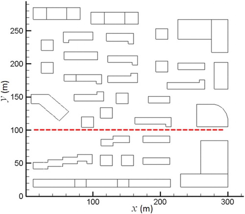
The physical model of the present study is based on the blueprint of a residential community located in the urban area of Hangzhou, China. The horizontal area is 350 m × 330 m in the x-y plane, containing 32 buildings (Figure 1). Each building has its own configuration and dimensions, with the heights varying from 12 m to 33 m (referred to as H_max hereafter). To retain the details of the real community as much as possible, the configuration of each building has been reconstructed carefully, even including the attic slope roof and ‘protruding part’. The computation domain is taken as 1350 m (x) × 1330 m (y) × 200 m (z), with a horizontal distance of 15H_max m away from the outer boundary of the community area and a vertical distance of 6H_max m away from the bottom ground. The maximum blockage ratio is below 3%, which is consistent with the suggestion of classic guidelines (Franke et al., 2004; Tominaga et al., 2008).

Figure 1. Top view of the residential community located in Hangzhou city. The dashed red line (y = 100 m, z = 1.6 m) represents the line to abstract data for comparisons.

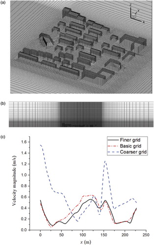
The grid system used for the simulation was generated using the commercial software Gambit (Figure 2). The whole computational domain is divided into two major parts: the inner part, including the community area, and the outer part, representing the surroundings. To strike a balance between the computational cost and numerical precision, finer grids were generated for the inner part at a resolution of 2 m, and relatively coarse grids were generated for the domain away from the border of the inner part, with a growth factor of 1.1 for the basic grid case. As the community area is quite complex, it was divided into small parts so that hexahedral grids could be generated individually. To avoid low precision and large discretization errors, nodes on the common face of two conjoint sub-domains were designed to exactly match each other. Attic structures often create highly skewed elements which may result in numerical error and even failure in the grid generation. For these aspects, tetrahedral grids are utilized near the corners of the building. As a result, the maximum skewness of the grid system is about 0.59, and the aspect ratio ranges from 1.0 to 4.6. Different grid sizes were carefully designed and tested until the configurations of the buildings were represented by a reasonably fine grid system. Figure 2(c) shows the grid-sensitivity analysis of the predicted velocity distribution along a line in the domain, as marked in Figure 1. The basic grid case has about 3.2 million hexahedral cells and the measured maximum skewness is 0.593894. A finer grid case with a resolution of 1 m in the community area and 6.1 million cells in total, as well as a coarser grid case with about 1.3 million hexahedral cells, are included for comparisons. A uniform inflow with a velocity of 2 m/s is imposed as the boundary condition for this test simulation. It is clear that the difference in the velocity distribution along the line between the basic grid and the finer grid is quite small, while the coarser grid shows significant deviation with high fluctuation. This indicates that the basic grid case with a resolution of 2 m in the community area is fine enough for such simulations, and thus is used for the present study.

Figure 2. (a) Computational domain and horizontal grid, (b) grid distribution in the vertical direction, and (c) comparison of velocity distribution along the dashed line marked in Figure 1 between the basic grid, coarser grid and finer grid cases.

2.2. Mathematical model

In this study, air is considered an incompressible fluid with a constant density and kinematic viscosity. The realizable model (Shih, Liou, Shabbir, Yang, & Zhu, 1995) is used to simulate the flows for its better performance on presenting reverse flows and wake flows, which are often encountered in such configurations. The related governing equations read: (1) (2) (3) (4) where

In the above equations, u_i is the mean velocity component in tensorial form, is the turbulent fluctuating velocity, P is the averaged pressure, g is the gravitational acceleration, S_Mi is the additional momentum source exerted on the fluid by dust particles, k is the turbulent kinetic energy, G_k is the production term of k due to the mean velocity gradient, is the isotropic dissipation rate of turbulent kinetic energy, σ_i is the turbulent Prandtl number of k and , μ and μ_t are the kinetic viscosity and turbulent viscosity of the fluid, respectively, and are the fluid and particle density, respectively, is the particle velocity, d is diameter of the dust particle, is the particle Reynolds number based on the relative velocity and the particle diameter (Morsi & Alexander, 1972), and C_D is the drag coefficient.

The dispersed dust particles are individually traced in the Lagrangian framework by the discrete particle model. Because of the high density ratio of the dust to air , the possible force terms such as the pressure gradient, virtual mass and Basset forces can be neglected (Maxey & Riley, 1983). The collision between particles is also neglected based on the assumption of dilute flows. Considering only the Stokes drag force and the gravitational force, the momentum equation for a single dust particle can be expressed as: (5) where the modified Stokes drag force coefficient C_D is expressed as (Morsi & Alexander, 1972): (6) where a₁, a₂, and a₃ are constants that apply to smooth spherical particles. Values are as follows:

Once the particle velocity is obtained, Equation (7) is used to calculate the trajectory of the particle through integration of the velocity during the short time intervals: (7) where is the location of the particle.

The collision between particles and walls is considered by the reflection model. By default, the normal particle-wall impact restitution coefficient is set as 0.5 for the normal direction and 0.7 for the tangential direction.

2.3. Boundary conditions and solving procedure

The primary wind direction is due north (the y direction) corresponding to the typical local weather conditions of the urban area being subject to the sandstorm. At the inflow, the following logarithmic wind profile as a function of height is used: (8)

Considering the high wind speed and the turbulence generated by the strong interaction between the wind and upstream buildings, an isotropic turbulence is added to this profile. The atmospheric boundary friction velocity u_*, turbulent kinetic energy k and turbulence kinetic dissipation ε are calculated following Richards and Hoxey (1993). (9) (10) (11) where z₀ is the roughness length of the atmospheric boundary layer with a value of 0.02 m to represent grassland in the present study (Wieringa, 1993), C_μ is a constant with a value of 0.09, and is the Von Carman constant. 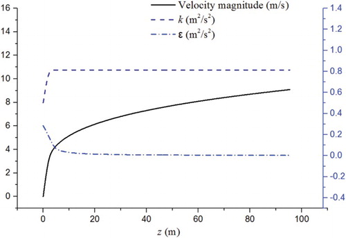I_U is determined by: (12) where z₀ = 0.02 m and B = 1 (ESDU, 1974). According to these parameters, the vertical profiles of the mean velocity U, turbulent kinetic energy k and turbulence kinetic dissipation ε at the inlet boundary are presented in Figure 3.

Figure 3. Vertical inflow profiles of the mean velocity, turbulent kinetic energy and dissipation rate.

At the outflow, the pressure outlet condition is applied with the static pressure set to zero. The top and lateral sides of the domain are assumed as being symmetric, and the non-slip boundary condition together with the standard wall function is applied to the bottom ground and the building surfaces. The surface roughness height K_s is considered and expressed using the following relationship (Blocken, Stathopoulos, & Carmeliet, 2007): (13)

K_s is set as 0.32643 m for the ground and 0.21762 m for the surface of buildings, corresponding to a surface roughness coefficient of C_s = 0.6 and 0.9, respectively. As the effect of upstream buildings is represented by the isotropic turbulence inlet condition, the ground roughness only takes the influence of grass with slight nonuniformity into consideration for simplification. Note that the type of lateral faces may be changed into inflow or pressure outlet boundary conditions for cases with different wind directions.

Dust particles are divided into nine different diameter groups based on the experimental results of Zhuang, Guo, Yuan, and Zhao (2001), and the Rosin–Rammler distribution is used to represent the statistic analysis of the particle size (Table 1). The particle density is estimated to be 2400 kg/m³ using the experimental data of W. Wang et al. (2005) with the assumption that all dust particles are ideal spheres. More than 80% of the mass fractions of these dust particles are within the range of PM10 and thus are treated as inhalable particles. The Stokes number of these particles is in the order of 0.001 based on the reference wind speed and maximum building height. Particles are injected into the computational domain with a mass flow rate that is calculated based on the production of normal components of the mean inflow wind velocity, inlet surface are and dust concentration (C) of the background (2.1e−6 kg/m³). To get a more realistic dust concentration field, the dust particles are injected into the domain in an unsteady way. Every 1000 time steps, a number of particles are released at the inflow boundary according to the mass flow rate. In total, about 3 million particle trajectories are tracked in the simulations.

Table 1. Sampled dust aerosol size distribution during the dust storm of the year 2000.

Diameter range (μm)	<0.4	<0.7	<1.1	<2.1	<3.3	<4.7	<5.8	<9.0
Concentration (μg·m^−3)	73.62	89.82	163.44	340.12	590.41	914.32	1208.78	1621.03
Content (%)	3.49	4.26	7.75	16.14	28.02	43.39	57.37	76.94

The commercial software FLUENT 6.3.26 is utilized as the flow solver. The convection terms of the momentum equation (Equation (2)), the turbulent kinetic energy equation (Equation (3)) and the turbulent kinetic energy dissipation rate equation (Equation (4)) are discretized using the QUICK scheme. The PRESTO scheme is employed for the pressure term while the SIMPLE algorithm is used to couple the pressure and velocity. The velocity and position of each particle are obtained by explicitly integrating Equation (5), while the effect of the particles on fluid is incorporated by taking the momentum exchange into account. The turbulent particle dispersion is considered using the discrete random walk model. Additional iterations were performed after the solution converged with a maximum residual threshold of 10⁻⁶ to ensure the global convergence. The parallel computation was carried out in a Linux environment with 32 CPUs, requiring about 6800 CPU hours to obtain reliable results for each case.

3. Numerical validation

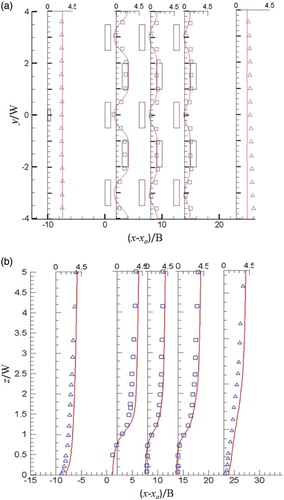
To validate the numerical method introduced above for such complex flows as the present study, the wind tunnel experiment conducted by Davidson, Snyder, Lawson, and Hunt (1996) was chosen as a benchmark. In the wind tunnel experiment, the staggered array consisted of 39 obstacles with dimensions of H = W = B = 0.12 m. The distance between the obstacles was twice the obstacle height, which was 0.24 m in both the streamwise (x) and spanwise (y) directions. The wind profile upstream of the arrays was characterized by a reference measurement at a height of 2H. At this point the ratio of the friction velocity (u_*) to the mean velocity (U) was 0.06 and the roughness height (z₀/H) was 0.0025. Flow-field measurements were made using both a hot-wire anemometer and a pulsed-wire anemometer. The hot-wire anemometer was used in the regions outside the obstacle array, while the pulsed-wire anemometer was used to make reliable measurements inside the obstacle array. In the present simulation, the physical configuration is taken to be the same as that of the experiment. The numerical models are taken to be the same as those presented in section 2. The computational domain covers 8.43 × 6 × 1.2 m³ resolved by a grid system of 225 × 180 × 40 along the three directions (Figure 4). The total grid number is about 1.45 million. The lateral and vertical profiles of the mean streamwise velocity at a z = H/2 horizontal plane and a y = 0 vertical plane are calculated and compared with those of the experimental data (Figure 5). It was found that the numerical lateral profiles of the mean streamwise velocity at z = H/2 horizontal plane are in good agreement with the experimental data, while deviations were observed in the vertical profiles, especially in the regions above the height of the obstacle. The reasons for this discrepancy may be related to the inflow boundary conditions and grid resolutions in the regions, as the profiles below the obstacle height are well predicted. These general consistent comparisons give us more confidence to present the numerical results for the community simulations in the next section.

Figure 4. Staggered obstacle array in the experiment and simulation for (a) the computational domain and (b) the grid settings.

Figure 5. Comparisons of mean streamwise velocity between the experimental data and the present simulation for (a) lateral profiles at the z = H/2 horizontal plane and (b) vertical profiles at the y = 0 vertical plane.

Note: □ = data measured with a pulsed-wire anemometer; △ = data measured with a hot-wire anemometer; red solid line = the present numerical results.

4. Results and discussion

4.1. The primary wind direction (north direction) condition

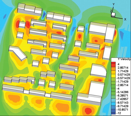
A due-north wind with a wind speed of 10 m/s⁻¹ at a reference height of 10 m was chosen as the default condition. As this inflow direction is perpendicular to the long axis of the community, it can be expected that the resulting flow field will be simpler than other inflow conditions, even though the inside flow field of the community is still complex (Figure 6). It is obvious that the buildings have a significant influence on the wind field. In the windward side of the community, the coming wind is blocked by three huge constructions, resulting in a relatively low wind speed. Between these huge constructions, several ‘corridors’ where the wind is accelerated and pushed into the community occur, illustrated by the blue and green colored parts in Figure 6. The blockage of the huge windward buildings and the channel flow in the corridors between these buildings are quite clear. A large proportion of wind flow enters the community through these corridors rather than the air ventilation between pedestrian and roof level. The pedestrian level wind velocity of these corridors can be comparable to the reference wind speed, represented by the blue part in Figure 6, resulting in a low wind speed environment. As these strong winds flow downstream, they are further influenced by the community layout. When impacting on downwind buildings, the flow is detached. A part of the channel flow is raised to the roof level, while the other still spins along the passages, resulting in spring-like streamlines in the passages between the buildings. In general, the wind speed in most parts of the community is below 5 m/s⁻¹ due to the blockage of the complex buildings, which helps to keep a relatively comfortable environment given the extreme weather conditions. Moreover, it is found that most regions of the community reserve a ‘positive’ wind speed (y direction) under the ‘negative’ prevailing wind direction condition (−y direction). These regions exist in the passages between the buildings with axes perpendicular to the wind direction or the leeward side of the downwind buildings. This is because when blocked wind flows through the passage, the strong shear stress causes vortex structures within the passages, just like the ‘skim type’ street canyon flow observed by Oke (1981).

Figure 6. The wind velocity distribution in the 1.6 m horizontal plane above the ground under the due-north wind condition case with a 10 m/s reference height wind velocity.

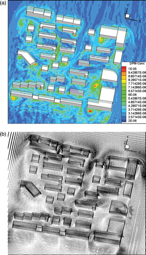
Few documents are available on the specific distribution of the dust concentration in the urban area. Maybe it is a common sense that dust distribution is dominated by the strong wind under this extreme weather conditions, but what interests us is to what extent its distribution is influenced by the presence of buildings. Figure 7 presents the dust concentration distribution on the horizontal plane of z = 1.6 m, together with the wind speed vector. It is obvious that the presence of buildings exerts remarkable influence on the dust concentration field. Most regions of the community keep a high dust concentration level (about twice that of the background concentration), because of the low wind speed resulting from the obstruction caused by the buildings. Another pronounced feature is that there are many ‘hot spots’, regions in which a high dust concentration that is as much as five times that of the background dust concentration is observed. These hot spots are usually located in the vortex core regions with very low wind speed (less than 1.5 m/s⁻¹) in the community. Dust is transported into these vortexes and circles around the vortex cores, leading to long residence time and such a high level of dust concentration. These vortexes are usually formed by flow separation just at the fringe of the leeward walls of buildings, similar to the flow reported in Davidson et al. (1996) and Tseng, Meneveau, and Parlange (2006). These observations indicate that harmfully high concentrations of dust particles may occur in complex urban areas, even if the inflow background concentration is lower.

Figure 7. Distribution of dust concentration under the due-north wind condition for (a) the wind velocity vector and (b) the 1.6 m horizontal plane above the ground.

The flow field and dust concentration are influenced not only by the horizontal layout of the buildings but also by their vertical structure. Figure 8 shows the dust concentration distribution in several vertical planes parallel to the primary due-north wind direction. As shown in Figure 8(a), two counter-rotating vortexes are formed between the first two buildings, and the lower one is anti-clockwise which causes the dust to concentrate on the windward side of the passage. In the passages between leeward buildings, one clockwise vortex is formed and the dust concentrates at the near ground corners. In the corridor between the tallest buildings shown in Figure 8(b), it is clear that the dust is accelerated and drawn into this region. After impacting with roofs, the dust is raised to flow over the buildings, which can be observed by the relatively high dust concentration above the downstream building roof. The dust distributions in the downstream passages resemble those of Figure 8(a), except for the passage with a large aspect ratio, for which a high dust concentration is found on both the windward and leeward sides. When the passage flow section area is blocked by internal building structures, a high wind speed occurs nearby but the dust still concentrates there. Such a situation can also be observed in the next downwind passage with a sharp change of the shape of the upwind building, where the leeward side of the passage causes a very high dust concentration level to occur.

Figure 8. Distribution of the dust concentration in several vertical planes parallel to the primary wind direction under the due-north wind condition for (a) x = 40 m, (b) x = 90 m, (c) x = 180 m, and (d) x = 240 m.

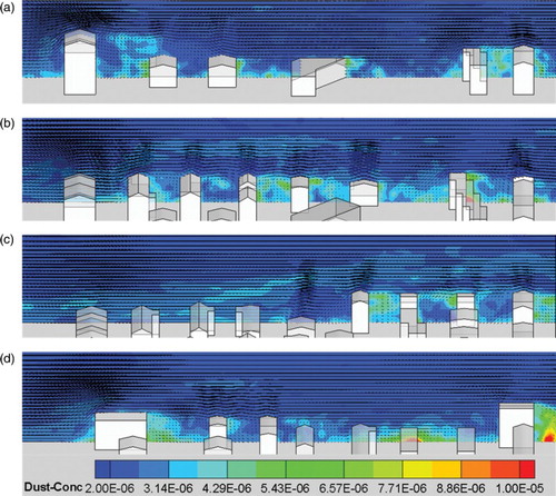
The sharp change of building shape may have a negative effect on the comfortability of the wind environment and the dust concentration at the pedestrian level in the present configuration, but the effect is different at the rooftop level. Comparing the triangular rooftop in Figure 8(c) with the regular rectangle one in Figure 8(d), the former can raise dust to a higher altitude so that it is easily blown out of the community by the upper wind, which helps to lower the dust load. Figure 8(d) further shows that a strong vortex can generate a high dust concentration region up to the height of the rooftop in the vicinity of the exit corridor between the ultimate south buildings.

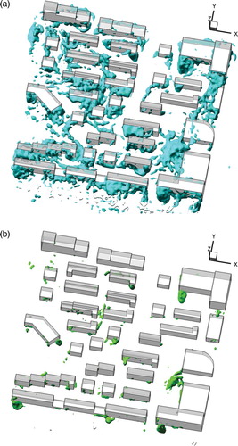
To show the global three-dimensional dust distribution in the community, the iso-surfaces of dust concentration of 4.2e−6 kg/m³ and 6.3e−6 kg/m³, which are two and three times the background concentration, respectively are presented in Figure 9. It is found that the accumulation effect of the dust particles is pronounced in the community. The accumulation area is mainly located in the passages (especially in the vicinity of the leeward wall) because of the relatively low velocity and inside strong vortex there, while the corridors preserve a low dust concentration level due to high velocity. Consequently, it seems to be difficult to maintain a region with both a low wind environment and a low dust concentration. As for the most seriously-affected regions, Figure 9(b) indicates that the most severe contamination in the community is located in the vicinity of the leeward fringe of the buildings and the regions with sharp change in the buildings’ shapes. These regions are covered by cores of vortexes and account for only a small part of the community.

Figure 9. Iso-surfaces of dust concentration under the due-north wind condition with values of (a) 4.2e−6 kg/m³ and (b) 6.3e−6 kg/m³.

4.2. Influence of the wind direction

Although the due-north wind is the local prevailing wind direction, it is worth to taking different wind directions into consideration. Accordingly, two more simulations with different wind directions, 30 degrees north by west (the northwest wind direction) and 30 degrees north by east (the northeast wind direction), were carried out.

4.2.1. The northwest wind direction condition

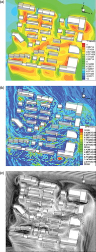
Figure 10 shows the distribution of the wind velocity field and dust concentration field in the 1.6 m horizontal plane above the ground under the northwest wind condition. As the wind direction changes 30 degrees to the west, the blockage effect of the huge northern buildings is compromised, decreasing the wind velocity in the corridors while increasing it inside the community. The west side of the community becomes another entrance of air flow while the east side becomes an exit. Affected by the approaching wind's x component velocity, the flow in the passages is forced to change direction to southeast. On the whole, the most direct influence comes from the wind flow entering from the west side. This part of the flow not only brings more air flux (resulting in a higher wind velocity) but also generates a channel flow along the passages, making the flow field more complex. An obvious example is that two counter-flows appear in the street canyon of the cambered main road – one from the north while the other form the west – and merge at the road's middle location, resulting in totally different flow conditions along the road. As for dust distribution, Figure 10(c) indicates that the dust accumulation becomes more pronounced in the vortex cores. Due to the special flow conditions along the cambered main road, different flow patterns appear in the middle of the community. In the vicinity of the merged area, numbers of vortexes and corresponding dust hot spots appear, while large areas with a high level of dust concentration are created in the north section.

Figure 10. Distribution of the y-component wind velocity under the northwest wind condition for (a) the wind velocity vector, (b) the dust concentration, and (c) the 1.6 m horizontal plane above the ground.

4.2.2. The northeast wind direction condition

In this case, all settings except the corresponding boundary conditions are the same as the northwest wind case (Figure 11). Under the northeast wind, the east side of the community serves as an entrance and the west serves as an exit. The ventilation of accumulated dust is significantly compromised not only by the relative small passage openings on the east side but also by the large angle between the passage axis and the wind direction (Figure 11(a)). Meanwhile, the lower entrance air flux reduces the inside ventilation level, the most obvious consequence of which is the large area of low wind velocity. The flow inside the passages is more or less distorted by the east flux, but the near-ground wind velocity is below 2 m/s⁻¹ and is similar to the previous two cases.

Figure 11. Distribution of the y-component wind velocity under the northeast wind condition for (a) the wind velocity vector, (b) the dust concentration, and (c) the 1.6 m horizontal plane above the ground.

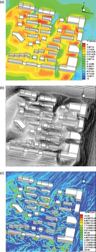
Although the wind environment maintains a relatively low level as a whole, the dust environment does not; the dust contamination condition is more serious, especially in the northwest part circled by the arc main road (Figure 11(c)). Because of the low wind speed and the complex flow conditions, the severe dust contamination of this region is inevitable. In the opposite southeast region, the contamination level is relatively low, as the building passages are almost linear to facilitate the transportation of the flux and dust.

These two cases suggest that the influence of the wind direction on fluid flow and dust distribution in an urban area are significant and should be taken into account when attempting to improve a community design.

4.3. Influence of particle-wall interactions

As so many walls are present in the computational domain, the particle-wall interactions are investigated in this section to study their influence on dust dispersion and distribution. Under the framework of the discrete particle model, two particle-wall interaction conditions – namely, ‘reflect’ and ‘capture’ – are applicable to the present study. For the reflect condition, the particle-wall impact restitution coefficient is of relevance, which may influence the numerical results according to a similar parameter study (Montazeri, Blocken, & Hensen, 2015). As the ideal elastic impact is unrealistic, three more different impact restitution coefficients are studied and the results are demonstrated in Figure 12. Here the north wind condition with a reference wind speed of 10 m/s⁻¹ is chosen as a benchmark.

Figure 12. Distributions of dust concentration in the 1.6 m horizontal plane above the ground under the due-north wind condition and with particle-wall impact restitution coefficient sets of: (a) normal 0.25, tangential 0.25, (b) normal 0.50, tangential 0.50, (c) normal 0.75, tangential 0.75, and (d) normal 0.50, tangential 0.7.

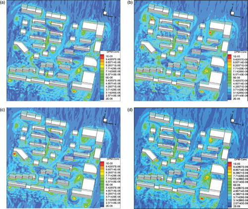
Generally speaking, these comparative cases result in the same dust distribution pattern and it is hard to tell the difference between them, especially for the low and moderate dust concentration regions. The most obvious difference lies in the concentration level of the hotspots; when the particle-wall impact restitution coefficient changes, the relatively high concentration regions surrounding these hotspots change slightly. This suggests that particle-wall collision does influence the particle transportation to some extent, but that the influence of the particle-wall impact restitution coefficient is not so great that a common assumed value of, say 0.5, would be suitable for the CFD simulation of the sandstorm.

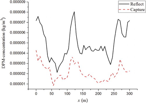
Under certain conditions, such as lower velocity and smaller particle size, the particles may be captured by the wall. To evaluate this effect, the capture condition is compared with the reflect condition for the northwest wind condition with a reference wind speed of 10 m/s⁻¹. Figure 13 shows the dust concentration distribution in the 1.6 m horizontal plane above the ground with the reflect and capture wall conditions. It is found that the dust concentration is generally largely reduced by the capture wall conditions, as expected. Note that here we capture all particles once they collide with the walls regardless of whether or not this happens in reality. Quantitatively, the averaged particle concentration under the reflect condition is about twice that of the capture condition, as shown in Figure 14 where the black line represents the reflect wall condition and the red line represents the capture wall condition. However, it is interesting to find that the use of different wall conditions does not change the general spatial variation trend of dust concentration in the community.

Figure 13. Distribution of dust concentration in the 1.6 m horizontal plane above the ground under the northwest wind condition for (a) the reflect wall condition and (b) the capture wall condition.

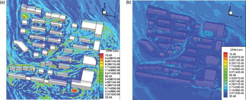
Figure 14. Spatial variation of particle concentration along the dashed line marked in Figure 1 under the reflection wall condition and the capture wall condition.

5. Conclusion

A Eulerian–Lagrangian CFD approach was used to investigate the wind field and dust distribution in a realistic residential community under a typical sandstorm weather condition. The flow was solved by a realizable model and the dust particles were tracked by a discrete particle model. It was found that the flow field in a real residential community is quite complex, and that the complexity may be increased by the construction layout and changes in the approaching wind direction. When the buildings axes are mainly perpendicular to the wind direction, the flows between the buildings basically resemble the classic street canyon flow. When the wind direction changes, the inside flow fields become more complicated. The dust distribution is closely related to the flow field. High levels of dust concentration areas with a low wind speed and high vorticity. The locations with the most severe dust contamination are those where vortexes appear and flow separation occurs. Building structures impose additional effects on the dust distribution. As the wind direction changes, the dust distribution differs from case to case, while the general features remain the same. Although the particle-wall interaction condition also influences the dust transportation, it does not change the spatial variation trend of the dust concentration in the community. It should be noted that the present study is limited by the artificial flow and dust boundary conditions. This could be addressed through coupling with meso-scale models to provide realistic boundary conditions in future studies. More realistic descriptions of particle-wall interactions are also needed to make the study more reliable.

Disclosure statement

No potential conflict of interest was reported by the authors.

Additional information

Funding

This work was supported by the Ministry of Environmental Protection of China [no. 201409008-4]; and the Zhejiang Provincial Key Science and Technology Project for Social Development [no. 2014C03025].

References

- Blocken, B., & Persoon, J. (2009). Pedestrian wind comfort around a large football stadium in an urban environment: CFD simulation, validation and application of the new Dutch wind nuisance standard. Journal of Wind Engineering and Industrial Aerodynamics, 97(5–6), 255–270. doi: 10.1016/j.jweia.2009.06.007
- Blocken, B., Stathopoulos, T., & Carmeliet, J. (2007). CFD simulation of the atmospheric boundary layer: Wall function problems. Atmospheric Environment, 41, 238–252. doi: 10.1016/j.atmosenv.2006.08.019
- Brunekreef, B., & Forsberg, B. (2005). Epidemiological evidence of effects of coarse airborne particles on health. European Respiratory Journal, 26(2), 309–318. doi: 10.1183/09031936.05.00001805
- Chu, P. C., Chen, Y. C., Lu, S. H., Li, Z. C., & Lu, Y. Q. (2008). Particulate air pollution in Lanzhou China. Environment International, 34(5), 698–713. doi: 10.1016/j.envint.2007.12.013
- Davidson, M. J., Snyder, W. H., Lawson, J. R. E., & Hunt, J. C. R. (1996). Wind tunnel simulations of plume dispersion through groups of obstacles. Atmospheric Environment, 30(22), 3715–3731. doi: 10.1016/1352-2310(96)00103-3
- ESDU. (1974). Characteristics of Atmospheric Turbulence near Ground. Part II: Single point Data for Strong Winds (Neutral Atmosphere). Item No. 74031, Engineering Sciences Data Unit, London.
- Fang, G. C., Chang, C. N., Wu, Y. S., Lu, S. C., Pi-Cheng, Fu P., Chang, S. C., … Yuen, W. H. (2002). Concentration of atmospheric particulates during a dust storm period in central Taiwan, Taichung. Science of the Total Environment, 287(1–2), 141–145. doi: 10.1016/S0048-9697(01)00996-2
- Franke, J., Hirsch, C., Jensen, A. G., Krüs, H. W., Schatzmann, M., Westbury, P. S., … Wright, N. G. (2004). Recommendations on the use of CFD in wind engineering, COST Action C14, Impact of Wind and Storm on City Life Built Environment.
- Garcia, S. A. P., Beeck, J. V., Rambaud, P., & Olivar, D. (2002). Numerical and experimental modelling of pollutant dispersion in a street canyon. Journal of Wind Engineering and Industrial Aerodynamics, 90(4–5), 321–339. doi: 10.1016/S0167-6105(01)00215-X
- Janhäll, S. (2015). Review on urban vegetation and particle air pollution–Deposition and dispersion[J]. Atmospheric Environment, 105, 130–137. doi: 10.1016/j.atmosenv.2015.01.052
- Maxey, M. R., & Riley, J. J. (1983). Equation of motion for a small rigid sphere in a nonuniform flow. Physics of Fluids, 26, 883–891. doi: 10.1063/1.864230
- Meng, Z. Q., & Lu, B. (2007). Dust events as a risk factor for daily hospitalization for respiratory and cardiovascular diseases in Minqin China. Atmospheric Environment, 41(33), 7048–7058. doi: 10.1016/j.atmosenv.2007.05.006
- Montazeri, H., Blocken, B., & Hensen, J. L. M. (2015). CFD analysis of the impact of physical parameters on evaporative cooling by a mist spray system. Applied Thermal Engineering, 75, 608–622. doi: 10.1016/j.applthermaleng.2014.09.078
- Morsi, S. A., & Alexander, A. J. (1972). An investigation of particle trajectories in two-phase flow systems[J]. Journal of Fluid Mechanics, 55(02), 193–208. doi: 10.1017/S0022112072001806
- Oke, T. R. (1981). Canyon geometry and the nocturnal urban heat island: Comparison of scale model and field observations. International Journal of Climatology, 1(3), 237–254. doi: 10.1002/joc.3370010304
- Richards, P. J., & Hoxey, R. P. (1993). Appropriate boundary conditions for computational wind engineering models using the k-ε turbulence model. Journal of Wind Engineering and Industrial Aerodynamics, 46&47, 145–153. doi: 10.1016/0167-6105(93)90124-7
- Sadiq, A.-B. M. A. R. (2014). CFD modeling of dust dispersion through Najaf historic city centre[J]. International Journal of Energy & Environment, 5(6), 723–728.
- Shao, Y., & Dong, C. H. (2006). A review on East Asian dust storm climate, modelling and monitoring. Global Planet Change, 52(1–4), 1–22. doi: 10.1016/j.gloplacha.2006.02.011
- Shih, T., Liou, W. W., Shabbir, A., Yang, Z., & Zhu, J. (1995). A new k-ϵ eddy viscosity model for high reynolds number turbulent flows. Computers & Fluids, 24(3), 227–238. doi: 10.1016/0045-7930(94)00032-T
- Song, Z. X. (2004). A numerical simulation of dust storms in China. Environmental Modelling and Software, 19(2), 141–151. doi: 10.1016/S1364-8152(03)00116-6
- Sun, J., Zhang, M., & Liu, T. (2001). Spatial and temporal characteristics of dust storms in China and its surrounding regions, 1901–1999: Relations to source area and climate. Journal of Geophysical Research-Atmospheres, 106(10), 325–333.
- Sun, J. H., Zhao, L. N., Zhao, S. X., & Zhang, R. J. (2006). An integrated dust storm prediction system suitable for east Asia and its simulation results. Global and Planetary Change, 52(1–4), 71–87. doi: 10.1016/j.gloplacha.2006.02.005
- Tominaga, Y., Mochida, A., Yoshie, R., Kataoka, H., Nozu, T., Yoshikawa, M., & Shirasawa, T. (2008). AIJ guidelines for practical applications of CFD to pedestrian wind environment around buildings. Journal of Wind Engineering and Industrial Aerodynamics, 96(10–11), 1749–1761. doi: 10.1016/j.jweia.2008.02.058
- Tseng, Y. H., Meneveau, C., & Parlange, M. B. (2006). Modeling flow around bluff bodies and predicting urban dispersion using large eddy simulation. Environmental Science & Technology, 40(8), 2653–2662. doi: 10.1021/es051708m
- Wang, W., Liu, H. J., Yue, X., Li, H., Chen, J. H., & Tang, D. G. (2005). Study on size distributions of airborne particles by aircraft observation in spring over eastern coastal areas of China. Advances in Atmospheric Sciences, 22(3), 328–336. doi: 10.1007/BF02918746
- Wang, X. M., Dong, Z. B., Zhang, J. W., & Liu, L. C. (2004). Modern dust storms in China: An overview. Journal of Arid Environments, 58(4), 559–574. doi: 10.1016/j.jaridenv.2003.11.009
- Wieringa, J. (1993). Representative roughness parameters for homogeneous terrain. Boundary-layer Meteorology, 63, 323–363. doi: 10.1007/BF00705357
- Xie, J. B., Yang, C. W., Zhou, B., & Huang, Q. Y. (2010). High-performance computing for the simulation of dust storms. Computers, Environment and Urban Systems, 34(4), 278–290. doi: 10.1016/j.compenvurbsys.2009.08.002
- Yoshie, R., Mochida, A., Tominaga, Y., Kataoka, H., Harimoto, K., Nozu, T., & Shirasawa, T. (2007). Cooperative project for CFD prediction of pedestrian wind environment in the Architectural Institute of Japan. Journal of Wind Engineering and Industrial Aerodynamics The Fourth European and African Conference on Wind Engineering, 95(9–11), 1551–1578. doi: 10.1016/j.jweia.2007.02.023
- Zhao, L. N., & Zhao, S. X. (2006). Diagnosis and simulation of a rapidly developing cyclone related to a severe dust storm in East Asia. Global and Planetary Change, 52(1–4), 105–120. doi: 10.1016/j.gloplacha.2006.02.003
- Zheng, D., Zhang, A., & Gu, M. (2012). Improvement of inflow boundary condition in large eddy simulation of flow around tall building[J]. Engineering Applications of Computational Fluid Mechanics, 6(4), 633–647. doi: 10.1080/19942060.2012.11015448
- Zhuang, G. S., Guo, J. H., Yuan, H., & Zhao, C. Y. (2001). The compositions, sources, and size distribution of the dust storm from China in spring of 2000 and its impact on the global environment. Chinese Science Bulletin, 46(3), 895–900. doi: 10.1007/BF02900460