Stage–discharge relationship for a pipe overflow structure in both free and submerged flow

ABSTRACT

Many facilities for urban drainage systems are equipped with a pipe overflow structure that can often be treated as a circular broad-crested weir. Thus it is possible to evaluate the overflow discharge through this device by measuring the water levels in the upstream tank and at the outlet of the pipe. In the present study, computational fluid dynamics (CFD) is used to determine a relationship between the discharge and the water levels upstream and downstream of the orifice for a range of diameters between 200 and 600 mm and a relative head up to 2. Over 50 numerical simulations are performed to take into account all the operating conditions of the system: free flow, submerged flow and pressurized flow. A regression is applied to the resulting data in order to obtain an orifice equation valid in both free-flow and submerged-flow regimes. Specific formulas, derived from Bernoulli's theorem, are also given for pressurized flows. The proposed methodology is applied to two examples.

KEYWORDS:

• Flow rate measurement
• numerical simulation
• stage–discharge relationship
• water level

1. Introduction

Many facilities used for drinking water supply or sanitation such as tanks, storm basins and pumping stations are equipped with an overflow, allowing them to divert excess inflow discharge of water into the receiving water (e.g., a natural river). When prescribed by legislation, the volume of diverted water must be monitored using appropriate instrumentation. One solution is to use water-level sensors in the facility to evaluate the volume discharged by the overflow using a hydraulic relationship between the water levels and the flow rate.

Generally, an overflow is composed of an orifice extended with a circular pipe. If the water level upstream of the orifice is largely above the top of the pipe, the flow is pressurized and a relationship between the flow rate and water levels can be calculated with Bernoulli's equation, taking into account friction losses and local head losses. In the case of open-channel flow, it is possible to set up a sharp-crested weir immediately upstream of the orifice. This weir implies a critical flow around the crest and enables the estimation of the discharge as a function of the upstream water level by using a classical relationship for a sharp-crested weir based on the geometry of the control section (Carlier, 1972; Geankoplis, 1983; Ghobadian & Meratifashi, 2012; Staus & Von Sanden, 1926; Streeter, 1966; Vantankhah, 2010). For example, the Hégly relationship (see Carlier, 1972) enables the estimation of the discharge over rectangular sharp-crested weirs with lateral contraction using the upstream water depth and the geometrical characteristics of the weir. But this kind of equipment is not necessary because the orifice and the upstream part of the circular pipe can be considered as a circular broad-crested weir in itself. Fewer experiments have been carried out on circular broad-crested weirs than on sharp-crested ones. Bos (1989) derived the head–discharge relationship for a circular broad-crested weir from Bernoulli's equation, assuming a hydrostatic pressure distribution above the crest (1) where is a discharge coefficient introduced to take into account neglected effects as streamline curvature (Bos, 1977), D is the orifice diameter, g is the standard acceleration due to gravity, and is a shape parameter for the control section. If the orifice diameter is known and the upstream head is set to a given value, the related value of can be deduced from the tables in Bos (1985). However the value is not well characterized, especially for relatively high heads for which streamline curvature has an increasing influence (Clemmens, Bos, & Replogle, 1984). Moreover, Equation (1) is valid if the critical regime occurs somewhere downstream of the weir but this cannot be guaranteed in all configurations, especially if the receiving water has an influence. Therefore, further investigations are necessary to derive a relationship between the water level upstream of the orifice (and possibly the water level downstream of it) and the discharge through the orifice, valid for both free flows – even with relatively high water levels – and submerged flows.

The complexity of the geometry and the different operating conditions of the system do not allow the determination of an analytical relationship. The study could have been conducted using an experimental approach (see, for example, Machiels, Erpicum, Archambeau, Dewals, & Pirotton, 2013; Machiels, Pirotton, Archambeau, Dewals, & Erpicum, 2014) but because of the large number of geometric configurations, computational fluid dynamics (CFD) is used. CFD has been successfully applied in a large number of similar studies to compute water–air flows for several types of hydraulic structure, including side weirs (Lipeme-Kouyi, 2004; Lipeme-Kouyi, Vazquez, Gallin, Rollet, & Sadowski, 2005), river flows (Chau & Jiang, 2001, 2004), broad-crested weirs (Hargreaves, Morvan, & Wright, 2007), combined sewer overflows (Chen, Han, Zhou, & Wang, 2013; Fach, Sitzenfrei, & Rauch, 2008), dam-break flows (Ozmen-Cagatay & Kocaman, 2011; Pu, Shao, Huang, & Hussain, 2013), Venturi flumes (Dufresne & Vazquez, 2013), and bottom spillways (Liu & Yang, 2014).

The results of the CFD simulations are summarized in the form of relationships (orifice equations) between the discharge and the water levels upstream and downstream of the orifice. These orifice equations must then be combined with the calculation of a backwater curve in the overflow pipe in order to build, point by point, a table linking the discharge with the water depths for the whole facility (orifice and pipe). The results obtained in this study are presented within the scope of sewage pumping station overflows, but they remain valid for other applications.

2. The hydraulic behavior of the system

An overflow pipe is made of a succession of two hydraulic elements: an orifice with a nozzle as an extension and a pipe that opens into the receiving water (Figure 1). The discharge drained away by the pipe, for a given water level in the tank, can be controlled by the orifice, the pipe or the combination of their respective effects.

Figure 1. Description of a pipe overflow structure.

2.1. At the orifice

For a particular facility, one or more operating conditions can occur, depending on the discharge. Different types of operating condition have been identified in order to link the water level in the tank – and also in some cases downstream of the orifice – with the discharge in the overflow pipe. At the orifice, four types of flow can be distinguished for such a system (Figure 2):

• Case 1a: open-channel flow with a transition from subcritical flow to supercritical flow.

• Case 1b: pipe flow upstream of the orifice and open-channel flow downstream of it, with a transition from subcritical flow to supercritical flow.

• Case 2: subcritical open-channel flow.

• Case 3: pressurized flow.

Figure 2. Different types of flow at the orifice.

2.1.1. Cases 1a and 1b: free flow

Cases 1a and 1b can be considered in a similar manner. They correspond to a subcritical flow upstream of the orifice and a supercritical flow downstream of it. Somewhere in between, the flow reaches the critical water level, which leads to a bijective depth–discharge relationship based on the critical flow theory. However, this is not easy to use in practice since the extent of the contraction and the positioning of the critical section within this contraction must be known in order to apply a simple calculation such as Bernoulli's equation. In contrast, the use of 3D modeling to reproduce the contraction phenomenon and the transition between subcritical flow and supercritical flow enables the determination of an orifice equation.

2.1.2. Case 2: submerged flow

The flow regime remains subcritical all the way between the upstream tank and the outfall. The water level downstream of the orifice influences the discharge and therefore the orifice equation has to be corrected for submerged flow. Case 2 also includes the following situation: a pipe flow at the orifice and a subcritical regime downstream.

2.1.3. Case 3: pressurized flow

Case 3 does not frequently occur in practice. Indeed the diameter of the overflow is generally chosen to avoid pressurized flows. Therefore the objective is to approximately evaluate the discharge. This can be approached as a classical hydraulic study: the water depth in the tank for a fixed discharge in the overflow pipe balances the head losses between the tank and the outlet of the pipe. In most cases, these head losses are a combination of a local head loss at the orifice and friction losses along the overflow pipe (Idel'cik, 1986). In some cases other local head losses have to be taken into account, for instance those induced by the downstream end of the pipe.

2.2. In the pipe

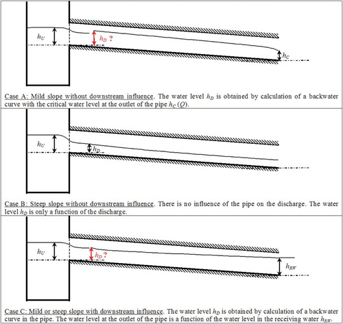
To obtain a relationship between discharges and water levels, it is necessary to take into account the characteristics of the pipe and eventually combine the orifice equations (derived from the numerical simulations) with a classical calculation of backwater curve in the pipe. Several operating conditions can be distinguished for the pipe, depending on the slope (mild or steep) and the potential influence of the receiving water downstream of the pipe (Figure 3). In cases A (a mild slope without downstream influence) and C (a mild or steep slope with downstream influence), the calculation of the backwater curve in the pipe is necessary to determine whether or not there the pipe or the receiving water are exerting an influencing on the discharge. The water level immediately downstream of the orifice is the distinguishing factor. In case B (steep slope without downstream influence), the discharge is only a function of the orifice diameter and the water level in the tank . More information on backwater curves can be found in Hager (1999).

Figure 3. Different types of flow in the pipe.

3. Materials and methods

3.1. The numerical model

Navier–Stokes equations are generally used to describe the motion of a fluid. For an incompressible fluid, these equations can be written as a mass conservation equation (Equation (2)) and a momentum conservation equation (Equation (3); Versteeg & Malalasekera, 2007): (2) (3) where is the fluid velocity, is the pressure, is the density, is the viscous stress tensor and is the body force.

The two-phase problem is solved using the volume of fluid method (Hirt & Nichols, 1981), which considers a single fluid (mixture), the properties of which vary as linear functions of the volume fraction . The mixture density, , and kinematic viscosity, , are expressed as (4) (5) where the subscripts and indicate water and air, respectively. The volume fraction is determined by solving the transport equation (6) where the third term on the left-hand side is an artificial compression term introduced in order to limit numerical diffusion and is a relative compression velocity (Rusche, 2002; Weller, Tabor, Jasak, & Fureby, 1998).

The equations above are solved using the two-phase incompressible flow solver interFoam, provided in the CFD software OpenFOAM (2015). A complete description of the model can be found in Deshpande, Anumolu, and Trujillo (2012). All numerical simulations were carried out under steady-state conditions. Since the objective of the numerical experiments was to compute the water level (not the variables linked to the anisotropy of the turbulence), the turbulence model k-ω SST (Shear Stress Transport) was chosen. The near-wall region is bridged using standard wall functions (ERCOFTAC, 2000).

3.2. The geometry, boundary conditions and grid analysis

The objective was to study different types of flow at the orifice; therefore, the simulation domain was composed of a rectangular tank with an orifice and the first meter of the overflow pipe (Figure 4). The method consisted in numerical experiments in which several discharges were set and the resulting water depths upstream and in some cases downstream of the orifice were computed. Several configurations were studied by varying the orifice and pipe diameters, but the following characteristics are common to all simulations:

• Rectangular tank of 1 m width and 1.5 m length.

• Circular pipe downstream of the orifice of 1 m length (1.5 m for Ø600).

• Slope: 0%.

Figure 4. Description of the simulation domain.

In reality, the slope of the pipe has an impact on the hydraulic behavior of the system. This is taken into account in the method using backwater curve calculations in the pipe. Since the aim of the numerical model was to study flows at the orifice and in the first part of the pipe, the length of the pipe was defined as being short (1 m or 1.5 m). For such lengths the influence of the slope is negligible, which has been checked by comparing the results obtained for slopes of 0% and 1%.

An inlet velocity was prescribed as the upstream boundary condition in order to prescribe the discharge. For the free flows, a pressure outlet was used as the downstream boundary condition. For the submerged flows, a water depth was imposed at the downstream end of the simulation domain. In both cases, the top of the domain was defined as a pressure outlet in order to reproduce atmospheric pressure. The free surface was defined as the surface corresponding to a 50% water volume fraction. The boundary conditions of the simulation domain are described in Figure 4.

All geometrical and hydraulic characteristics of the studied configurations are presented in Table 1. A total of 31 simulations corresponded to cases 1a and 1b (free flows), 3 simulations – for high flow rates – led to pressurized flows at the orifice (case 3), and 23 simulations corresponded to case 2 (submerged flows). For each case, the results of the simulations provide the position of the free surface (Figure 5).

Figure 5. Evolution of the free surface for the different cases by CFD.

Note: The values are as follows: case 1a, 400 mm diameter and 50 l/s; case 1 b, 250 mm diameter and 75 l/s; case 2, 500 mm diameter and 60 l/s; case 3, 250 mm diameter and 100 l/s.

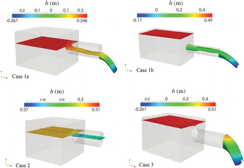
Table 1. Geometric and hydraulic characteristics of the studied configurations.

Free flow	Diameter D of the orifice (mm)	200	250	300	400		500	600
	Range of discharges (l/s)	1–40	1–100	1–100	1–220		23–243	10–605
	Number of simulations	5	7	7	8		4	5
Submerged flow	Diameter D of the orifice (mm)	300			500
	Simulated discharge (l/s)	5	10	25	50	23	60	84
	Range of (%)	41–97				58–99
	Number of simulations	3	4	3	2	4	4	3

The grid for the case where the pipe was of 300 mm diameter comprised almost 492,000 cells. In order to estimate the numerical uncertainty, one hydraulic configuration was simulated with a coarser mesh (about 393,000 cells) and the Grid Convergence Index (GCI) introduced by Roache (1994) was used: (7) where is the value of the grid ratio (here 1.25), is equal to 2 for a second-order method, is the result obtained for a fine grid (492,000 cells), and is the result obtained for the coarse grid. The computed water levels in the tank are compared for the two grids. The analysis led to an estimated numerical uncertainty of about 4% for the fine grid.

4. Results and discussion

4.1. Computed water levels

In the case of free flows, the total head over a cross-section was calculated in different transverse planes along the overflow pipe. For each simulation, a chart representing the evolution of the total head in the direction of the flow was created (Figure 6). For a negative abscissa, the value corresponds to the total head in the upstream tank, which is considered as equal to the water depth given that the kinetic component is negligible compared to the water level. The abscissa corresponds to the inlet of the pipe (orifice) and corresponds to the outlet of the pipe.

Figure 6. Evolution of the hydraulic head for a pipe with a diameter of 500 mm and a discharge of 84 l/s.

The water depth upstream of the orifice is an average of the water depths computed in the tank, given that the water level does not vary much (3% between the minimum and maximum values). It is measured from the invert of the pipe. The water level is computed where the total head reaches a uniform value ( in Figure 6). It corresponds to the area where the local head loss caused by the orifice entirely dissipates. Then the total head loss consists only of friction losses, which are negligible compared to the local head losses. This area was located in the first meter of the pipe for all simulations. It should be highlighted that is the water level just downstream of the orifice (and not that of the receiving water).

For submerged flows, was set as a downstream boundary condition; only the water level in the upstream tank was obtained from the simulations.

Finally, the following dimensionless variables are introduced for each numerical experiment:

• , as defined by Hager (1999) and corresponding to a relative discharge for a circular pipe.

• ; ; , where is the orifice diameter.

4.2. Validation of the numerical model

The results of the 25 numerical simulations under free flow conditions with between 0 and 1 (case 1a) were compared to the relationship proposed by the United States (US) Department of Transport for highway culverts (US DoT, 2012). Indeed their geometries are similar to those of overflow pipe structures when the upstream water level is lower than the culvert diameter. Based on model tests of the weir geometry and measurement of prototype discharges, the following relationship between flow and water-surface elevation was developed for unsubmerged inlet control flow: (8) where is the headwater depth above the inlet control section, is the interior height of the culvert barrel, and are constants depending on the geometry, is a constant for unit conversion (1.811 SI), is the discharge and is the full cross-sectional area of the culvert barrel. For a circular rough tapered inlet throat, the values of and are 0.519 and 0.64, respectively (US DoT, 2012).

Figure 7 shows a comparison between the numerical simulations and the relationship proposed by the US DoT (2012), expressed in terms of dimensionless discharge as a function of dimensionless upstream water level . The numerical results are in good agreement with the relationships previously described and therefore it can be concluded that the interFoam solver is usable to simulate flows through the orifice.

Figure 7. Comparison between numerical experiments and the US DoT (2012) relationship for case 1a.

4.3. Analysis of flows at the orifice

4.3.1. Cases 1a and 1b: free flow

Figure 8 represents the evolution of the dimensionless discharge as a function of the dimensionless upstream water depth for 31 simulations under free flow conditions (below the dashed line). An interpolation function was developed that expresses the discharge for a free flow as a function of the upstream water level h_U, knowing the diameter . The maximum error between Equation (9) and the CFD data is 4%: (9)

Figure 8. Evolution of the dimensionless discharge versus the upstream dimensionless water depth for free flows.

Three additional simulations were carried out in order to determine the limit above which the flow becomes pressurized. This limit was evaluated to or , so Equation (9) is valid when . This value should be considered as an approximate limit. For example, it is probable that this value is different when the discharge is increasing from when it is decreasing (hysteresis). Further developments would be needed to precisely evaluate this transition.

4.3.2. Case 2: submerged flow

For each simulation under submerged flow conditions, the discharge and the downstream water depth were prescribed while the upstream water depth was computed. From the upstream water depth, the potential discharge if the flow is not submerged can be evaluated using Equation (9). The variable was plotted against (Figure 9), leading to the fitting of the following interpolation: (10)

Figure 9. Evolution of versus for submerged flows.

The modular limit (between free and submerged flows) can be approximately evaluated to using Figure 9. Indeed, the ratio is close to 1 when < 0.73. For < 0.97, the maximum error with respect to the simulated discharge is 6%. In the range between 0.97 and 1, the maximum error equals 40%. However, when is more than 0.97, the difference between the two water levels is small and the measurement uncertainty becomes very significant. Consequently, the method based on water-level sensors cannot be used in this range of water depths. Equation (10) is valid for and .

4.3.3. Case 3: pressurized flow

Since case 3 is not frequent, the following equations provide only an approximate estimation of the discharge. In this context, the relationship between the discharge and the water levels in the tank and of the receiving water can be given by the Bernoulli equation. Two cases can be distinguished. The first corresponds to an influence on the flow exerted by the receiving-water level. The second can be seen as a free jet of which the head can be approximated by (atmospheric pressure and potential head equal to half the diameter), where D is the diameter of the pipe and v is the velocity of the fluid. In both cases, an analytical formula is obtained giving the discharge as a function of or of the pair .

If , i.e., the the receiving-water level influences the flow, then the discharge is calculated using (11) while if there is no influence exerted by the receiving-water level, the discharge is calculated using (12) where is the section of the pipe of diameter : , is the hydraulic radius = , and are the head loss coefficients at the orifice and the outlet of the pipe (Idel'cik, 1986), is the Strickler roughness coefficient of the pipe, and and are the slope and length of the pipe, respectively.

4.3.4. Overall method

The flow chart in Figure 10 summarizes the method used to determine the stage–discharge relationship for a given pipe overflow structure. The operating conditions of the hydraulic system, and consequently the relationship which is to be used, are evaluated as a function of the discharge and the water depths.

Figure 10. Flow chart for determining the type of flow as a function of the discharge and the water depths.

In Figure 11, the dimensionless discharges in the cases of the free flows and submerged flows are plotted against the dimensionless upstream water level and the difference . The limits of the submerged flow with the free flow and the pressurized flow are also highlighted in Figure 11. The dimensionless discharges are only represented for the range .

Figure 11. Dimensionless discharges versus dimensionless upstream water depth and .

5. Examples

The two following examples show the use of the proposed method to derive a depth–discharge relationship for a given structure. The first is comprised of an overflow pipe without the influence of the pipe on the discharge (steep slope) and the second is comprised of an overflow pipe with the influence of the pipe on the flow rate (mild slope).

5.1. Example 1

The geometrical characteristics of the pipe considered in this example are as follows: .

The first step is to determine the maximum discharge and maximum water level in the tank in the case of a free flow through the orifice: and . The maximum discharge under free-flow conditions is 222 l/s for a water level of 0.68 m in the tank. This overflow pipe has a steep slope, i.e., the flow is supercritical in a range between 0 and 287 l/s for steady-state and uniform conditions. The upper limit is higher than the maximum flow rate under free-flow conditions. The 0.68 m value is then higher than the critical water level for any flow rate under free-flow conditions. Provided that the level of the receiving water remains sufficiently low, it has no influence and the discharge is given by Equation (9) while .

In the case of a pressurized flow, Equation (12) must be used. Figure 12 shows the evolution of the discharge versus the upstream water level . There is a discontinuity in the zone where the flow becomes pressurized (Kerger, Erpicum, Dewals, Archambeau, & Pirotton, 2011), which corresponds to a transition zone where the evaluation of the flow rate is less accurate.

Figure 12. Relationship between the discharge and the water level in the tank for free flow.

The relationship presented in Figure 12 is only valid if the water level upstream of the pipe is not influenced by the receiving-water level. The receiving-water levels for which the limit is reached have to be calculated for each discharge. The graph in Figure 13 was constructed by varying the upstream water level between 0 and 0.56 m. The discharge in free-flow conditions was calculated for each water level and then the receiving-water level was calculated using a backwater curve in the overflow pipe so that . To ensure that the flow remains free, the receving-water level must be lower than the limits shown in Figure 13.

Figure 13. Limits between free flows and submerged flows.

5.2. Example 2

Example 2 corresponds to a mild slope pipe with the following geometrical characteristics: .

According to Equation (9), the maximum discharge under free-flow conditions is 108 l/s for a water level of 0.51 m in the tank. As the pipe has a mild slope, it is necessary to check if is lower or higher than . Table 2 was constructed by varying the water level upstream between 0 and 0.51 m, with the discharge in free-flow conditions for each water level. The water level downstream of the orifice was calculated using a backwater curve in the overflow pipe. The outlet boundary condition is considered as a free outlet that is not influenced byt the receiving-water level so that the water level at the outlet reaches the critical water level.

Table 2. Verification of the submerged conditions at the orifice as a function of the water level upstream.

hU (m)	QF (m^3/s)	hD (m)	0.73 × hU (m)
0.05	0.002	0.05	0.04
0.10	0.008	0.09	0.07
0.20	0.029	0.18	0.15
0.30	0.055	0.27	0.22
0.35	0.069	>0.30	0.25
0.40	0.082	>0.30	0.29
0.51	0.108	>0.30	0.37

Table 2 shows that the condition is verified for all discharges so that the orifice is always submerged. ThereforeEquation (10) can be used to calculate the discharge (Figure 14). Because of backwater effect, the flow becomes pressurized above 55 l/s (and not 108 l/s, as previously evaluated under free-flow conditions), in which case Equation (12) applies.

Figure 14. Relationship between the discharge and the water level in the tank for submerged flow.

6. Conclusion

This study aimed to determine stage–discharge relationships for the evaluation of the volume discharged by an overflow pipe. Hydraulically speaking, the orifice and the nozzle can be considered as a broad-crested circular weir. The different operating conditions at the orifice were studied in more than 50 numerical simulations in order to obtain orifice equations that are valid for both free and submerged flows. These relationships can be used for a range of diameters between 200 and 600 mm and a dimensionless upstream water level of up to 1.7. The modular limit between the free flows and submerged flows was found to be approximatively . Further simulations around this value would be necessary to better identify the modular limit. The orifice equations must then be combined with backwater curve calculations in the pipe in order to build a stage–discharge relationship for the whole facility. Specific formulas, derived from Bernoulli's theorem, are also given for pressurized flows. The limit between open-channel flows and pressurized flows at the orifice was found to be around , but further investigation is needed to precisely determine this value.

Taking into account the numerical uncertainty and the error in the fit between interpolation functions and CFD data, the uncertainty of the orifice equation is about 5% for free-flow conditions and about 10% for submerged-flow conditions for values of < 0.97. These values do not take into account the measurement uncertainty on the water level, which depends on the technology used. The derived relationships are readily available for real-world engineering applications, such as the self-monitoring of sewer networks.

Acknowledgments

This work is part of two national projects, Computations and their Applications in Channel Hydraulics for Sewers (COACHS) and MENTOR.

Disclosure statement

No potential conflict of interest was reported by the authors.

References

- Bos, M. G. (1977). The use of long-throated flumes to measure flows in irrigation and drainage canals. Agricultural Water Management, 1, 111–126. doi: 10.1016/0378-3774(77)90035-X
- Bos, M. G. (1985). Long-throated flumes and broad-crested weirs. Dordrecht, The Netherlands: Nijhoff.
- Bos, M. G. (1989). Basic principles of fluid flow as applied to measuring structures. In M. G. Bos (Ed.), Discharge measurement structures (pp. 17–65). Wageningen, The Netherlands: ILRI.
- Carlier, M. (1972). Hydraulique générale et appliquée [General and applied hydraulics]. Paris: Eyrolles.
- Chau, K. W., & Jiang, Y. W. (2001). 3D numerical model for pearl river estuary. Journal of Hydraulic Engineering, 127(1), 72–82. doi: 10.1061/(ASCE)0733-9429(2001)127:1(72)
- Chau, K. W., & Jiang, Y. W. (2004). A three-dimensional pollutant transport model in orthogonal curvilinear and sigma coordinate system for Pearl river estuary. International Journal of Environment and Pollution, 21(2), 188–198. doi: 10.1504/IJEP.2004.004185
- Chen, Z., Han, S., Zhou, F. Y., & Wang, K. (2013). A CFD modelling approach for municipal sewer system design optimization for minimize emissions into receiving water body. Water Resources Management, 27, 2053–2069. doi: 10.1007/s11269-013-0272-9
- Clemmens, A. J., Bos, M. G., & Replogle, J. A. (1984). RBC broad-crested weir for circular sewers and pipes. Journal of Hydrology, 68, 349–368. doi: 10.1016/0022-1694(84)90220-8
- Deshpande, S. S., Anumolu, L., & Trujillo, M. F. (2012). Evaluating the performance of the two-phase flow solver interFoam. Computational Science & Discovery, 5, 014016–014052. doi: 10.1088/1749-4699/5/1/014016
- Dufresne, M., & Vazquez, J. (2013). Head-discharge relationship of Venturi flumes: From long to short throats. Journal of Hydraulic Research, 51(4), 465–468. doi: 10.1080/00221686.2013.781550
- ERCOFTAC. (2000). Best practice guidelines, Version 1.0 (M. Casey & T. Wintergerste, Eds.). ERCOFTAC Special Interest Group on Quality and Industrial CFD.
- Fach, S., Sitzenfrei, R., & Rauch, W. (2008). Assessing the relationship between water level and combined sewer overflow with computational fluid dynamics. Proceedings of the 11th International Conference on Urban Drainage, Edinburgh, Scotland, UK.
- Geankoplis, C. J. (1983). Transport processes and unit operations. Englewood Cliffs, New Jersey: Prentice-Hall.
- Ghobadian, R., & Meratifashi, E. (2012). Modified theoretical stage-discharge relation for circular sharp-crested weirs. Water Science and Engineering, 5(1), 26–33.
- Hager, W. H. (1999). Wastewater hydraulics. Berlin, New York: Springer.
- Hargreaves, D. M., Morvan, H. P., & Wright, N. G. (2007). Validation of the volume of fluid method for free surface calculation: The broad-crested weir. Engineering Applications of Computional Fluid Mechanics, 1(2), 136–146. doi: 10.1080/19942060.2007.11015188
- Hirt, C. W., & Nichols, B. D. (1981). Volume of fluid (VOF) method for the dynamics of free boundaries. Journal of Computational Physics, 39, 201–225. doi: 10.1016/0021-9991(81)90145-5
- Idel'cik, I. E. (1986). Mémento des pertes de charge [Handbook of energy losses]. Paris: Eyrolles.
- Kerger, F., Erpicum, S., Dewals, B. J., Archambeau, P., & Pirotton, M. (2011). 1D unified mathematical model for environmental flow applied to steady aerated mixed flows. Advances in Engineering Software, 42(9), 660–670. doi: 10.1016/j.advengsoft.2011.04.012
- Lipeme-Kouyi, G. (2004). Expérimentations et modélisations tridimensionnelles de l'hydrodynamique et de la separation particulaire dans les déversoirs d'orage. PhD thesis, Université de Strasbourg.
- Lipeme-Kouyi, G., Vazquez, J., Gallin, Y., Rollet, D., & Sadowski, A. G. (2005). Use of 3D modelling and several ultrasound sensors to assess overflow rate. Water Science and Technology, 51(2), 187–194.
- Liu, T., & Yang, J. (2014). Three-dimensional computations of water – Air flow in a bottom spillway during gate opening. Engineering Applications of Computational Fluid Mechanics, 8(1), 104–115. doi: 10.1080/19942060.2014.11015501
- Machiels, O., Erpicum, S., Archambeau, P., Dewals, B., & Pirotton, M. (2013). Parapet wall effect on piano key weir efficiency. Journal of Irrigation and Drainage Engineering, 139(6), 506–511. doi: 10.1061/(ASCE)IR.1943-4774.0000566
- Machiels, O., Pirotton, M., Archambeau, P., Dewals, B., & Erpicum, S. (2014). Experimental parametric study and design of Piano Key Weirs. Journal of Hydraulic Research, 52(3), 326–335. doi: 10.1080/00221686.2013.875070
- OpenFOAM. (2015). User guide (2nd ed.). OpenCFD Ltd.
- Ozmen-Cagatay, H., & Kocaman, S. (2011). Dam-break flow in the presence of obstacle: Experiment and CFD simulation. Engineering Applications of Computational Fluid Mechanics, 5(4), 541–552. doi: 10.1080/19942060.2011.11015393
- Pu, J. H., Shao, S., Huang, Y., & Hussain, K. (2013). Evaluations of SWEs and SPH numerical modelling techniques for dam break flows. Engineering Applications of Computational Fluid Mechanics, 7(4), 544–563. doi: 10.1080/19942060.2013.11015492
- Roache, P. J. (1994). Perspective: A method for uniform reporting of grid refinement studies. Journal of Fluids Engineering, 116, 405–413. doi: 10.1115/1.2910291
- Rusche, H. (2002). Computational fluid dynamics of dispersed two-phase flows at high phase fractions. Ph.D. Thesis, Imperial College of Science, Technology and Medicine, London.
- Staus, A., & Von Sanden, K. (1926). Der kreisrunde Überfall und seine Abarten. München: Oldenbourg.
- Streeter, V. L. (1966). Fluid mechanics. New York: McGraw-Hill.
- U.S. Department of Transportation, Federal Highway Administration. (2012). Hydraulic design series, Number 5, Hydraulic Design of Highway Culverts, Third Edition.
- Vantankhah, A. R. (2010). Flow measurement using circular sharp-crested weirs. Flow Measurement and Instrumentation, 21, 118–122. doi: 10.1016/j.flowmeasinst.2010.01.006
- Versteeg, H. K., & Malalasekera, W. (2007). An introduction to computational fluid dynamics: the finite element method. Harlow, England: Prentice-Hall.
- Weller, H. G., Tabor, G., Jasak, H., & Fureby, C. (1998). A tensorial approach to computational continuum mechanics using object oriented techniques. Computers in Physics, 12(6), 620–631. doi: 10.1063/1.168744