Numerical simulations of the mean wind speeds and turbulence intensities over simplified gorges using the SST k-ω turbulence model

ABSTRACT

Numerical studies on the wind characteristics over gorge and valley terrains are very rare. Some simplified gorge terrains with different included angles and different terrain heights were adopted in the present study in order to obtain the basic information about the wind characteristics. To ensure the accuracy of the numerical results before conducting the actual numerical simulations, a new form of turbulence kinetic energy profile to serve as an inlet boundary condition was proposed based on the SST k-ω turbulence model. Then, the wind characteristics – including the mean wind speeds, turbulence intensities and mean square deviations – of the turbulent flow in the gorge terrain were studied for different included angles and different terrain heights. The results showed that the larger the included angle of the gorge terrain, the more significantly the mean wind speeds at the gorge center increase. The mean square deviation values of the turbulent flow at the gorge center are much smaller than those at the inlet. The effects of the terrain height on wind characteristics such as the mean wind speed and turbulence intensity at the gorge center are very small. The research conclusions can provide a point of reference for the wind characteristics over real gorge terrain and the simulation method of the current study can provide a new idea for other numerical simulations.

KEYWORDS:

• Simplified gorge
• computational fluid dynamics
• boundary conditions
• equilibrium atmospheric boundary layer
• mean wind speed
• turbulence intensity

1. Introduction

Computational wind engineering is one of the most promising research directions for structural wind engineering, of which the core is computational fluid dynamics (CFD). Compared with traditional methods such as field measurements and wind tunnel tests, the CFD numerical simulation method has many advantages, including easy modeling, convenient control, and the changing and repeating of the test conditions, as well as being able to give quantitative results. With the ongoing advancement of numerical solution methods and computer hardware, the application of the CFD numerical simulation method to structural wind engineering has become an important subject for study, and it is more and more widely used in the numerical simulation of wind characteristics over complex terrain (Cao, Wang, Ge, & Tamura, 2012; Y. L. Li, Hu, Cai, Tang, & Liao, 2011; Maurizi, Palma, & Castro, 1998; Tamura, Okuno, & Sugio, 2007).

For the numerical studies on the wind characteristics over two-dimensional and three-dimensional complex terrains, Iizuka and Kondo (2004, 2006), Wan, Porté-Agel, and Stoll (2007) and Cao et al. (2012) studied the turbulent flow over a two-dimensional steep hill using a large-eddy simulation (LES) turbulence model and compared the numerical results with those obtained from a wind tunnel test. The results of these studies showed that when using the appropriate sub-grid scale (SGS) model and other parameters in the simulations, the numerical results were in very good agreement with the experimental data obtained from wind tunnel tests. Tamura et al. (2007) investigated turbulent boundary-layer types of flow over a three-dimensional, steep, hill-shaped model using the LES method and discussed the effects of the surface condition of a hill, such as vegetation effects, by using the feedback forcing method. The numerical results showed sufficiently good agreement with the mean wind speed and turbulence intensity obtained from wind tunnel tests for both smooth and rough surfaces. In particular, the degree of deceleration due to vegetation corresponded to the test results well. The computed and test peak heights of turbulence intensity were also in a good agreement for both the smooth and rough test conditions. Based on the Reynolds-averaged Navier–Stokes (RANS) method, Hu, Li, Cai, Liao, and Xu (2013) proposed a set of inlet boundary conditions by using the SST k-ω turbulence model and derived the source terms for k and ω to satisfy their corresponding transport equations. According to this method, the equilibrium atmospheric boundary layer (ABL) was satisfactorily achieved in an empty computational domain and an actual numerical simulation on the wind characteristics over a two-dimensional trapezoidal hill was further conducted. The results showed that the proposed inlet profiles and source terms needed to achieve an equilibrium ABL can greatly improve the accuracy of the actual numerical simulation.

For the numerical studies on the wind characteristics over real three-dimensional complex terrain, Kim, Patel, and Lee (2000) simulated the wind flow over a hilly terrain based on the two-equation turbulence models together with the wall functions to account for the effects of surface roughness. The numerical predictions at four sites were found to be in reasonable agreement with the field measurements with respect to the wind magnitude and flow separation when presented. Maurizi et al. (1998) carried out a numerical simulation of the wind flow over a mountainous area in a horizontal region of 15 km × 14 km, and discussed the effects of grid resolution and flow inlet conditions on the wind flow over it. The results showed that it was possible to obtain three-dimensional simulations of the atmospheric flow over complex terrain within a reasonable amount of computer time, and differences of about 10% of the wind speed measured 30 m above the ground occurred as a result of different grid resolutions and flow inlet conditions. Uchida and Ohya (2003) carried out the calculation of turbulent flow over a real complex terrain in a horizontal region of 9.5 km × 5 km with a relatively fine spatial resolution of 50 m and calculated the unsteady flow field caused by the upstream roughness blocks to generate instantaneous velocity fluctuations in the approaching flow. The results showed that the wind field in the central region of the research area was strongly influenced by the wake region generated behind a high mountain, while the airflows moving around the side of the mountain exhibit relatively small fluctuations.

It should be pointed out that the overwhelming majority of numerical studies on the wind characteristics over complex terrain are aimed at hilly or mountainous terrain as discussed above, while numerical studies on the wind characteristics over gorge and valley terrain are very rare. Long-span bridges located in complex terrain typically straddle deep-cutting gorges, so it is both necessary and important to investigate the wind characteristics over such terrain in order to improve the effectiveness and safety of the wind-resistant designs used for these bridges (C. G. Li, Chen, Zhang, & Cheung, 2010; Y. L. Li et al., 2011; Zhu, Ren, Chen, Zhou, & Wang, 2011). Furthermore, when studying the air pollution in valley terrain (Sierputowskia, Ostrowskia, & Cenedeseb, 1995) and studying the development of aeolian bedforms and processes of aeolian sedimentation in valleys (Bullard, Wiggs, & Nash, 2000), more studies of the wind characteristics over gorge and valley terrain are needed. In such circumstances, carrying out numerical studies on the wind characteristics over gorge and valley terrain can not only make full use of the advantages of the numerical simulation method to better explore the change law of the wind characteristics over gorge and valley terrain, but they also can extend the numerical simulation method to more complex types of terrain and other fields.

However, there are two issues when using the numerical simulation method to investigate the wind characteristics over gorge and valley terrains. Firstly, since each real gorge and valley has a unique geometric shape, the wind characteristics will vary; thus, each study on the wind characteristics over a real area of gorge or valley terrain is a single-case study that will have limited value in terms of generalization. To avoid the limitations of single-case studies on wind characteristics, an area of simplified gorge or valley terrain can be introduced in order to obtain the basic information about the wind characteristics over such terrains (Bullard et al., 2000; C. G. Li et al., 2010; Sierputowskia et al., 1995). Furthermore, the basic information obtained about an area of simplified gorge or valley terrain can also contribute to understanding the complex wind characteristics over real gorge and valley terrains. Secondly, as the accuracy of the numerical results are usually validated by wind tunnel tests or field measurements, the inlet boundary conditions of the computational domain should be kept the same as those of the wind tunnel tests or field measurements, but achieving this is very difficult (Cao et al., 2012; Hu et al., 2013). Zheng, Zhang, and Gu (2012) presented a set of inflow boundary conditions based on the LES method to ensure that the simulated oncoming wind field of the computational domain coincided with those of the wind tunnel test, and this method was adopted to simulate the wind field around a single tall building. Liu (2012) presented another set of inflow boundary conditions based on the digital filter technique in order to realize the inflow turbulence on the inlet of the computational domain, and used these conditions to investigate the wind characteristics around a square cylinder. Although the above research could provide a point of reference for solving the issue of the inlet boundary conditions of the computational domain, the accuracy of their numerical results and the efficiency of their method should be further improved. The inlet boundary conditions of the computational domain have in fact become an important unresolved issue in CFD research (Liu, 2012). In particular, it has become a very important factor that influences the accuracy of the results of numerical simulations (Blocken, Carmeliet, & Stathopoulos, 2007).

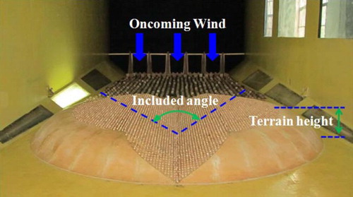
With the above problems and previous studies in mind, areas of simplified gorge terrain were introduced in the present study and numerical simulations on the wind characteristics over them were conducted by employing CFD using the commercial software FLUENT (Fluent Inc., 2006) to obtain fundamental information that can potentially be generalized to understand the effects caused by gorge terrain geometry. To ensure the accuracy of the numerical results prior to conducting the actual numerical simulations, a new form of turbulence kinetic energy profile to serve as an inlet boundary condition was proposed based on the SST k-ω turbulence model, and this was proved to be very effective by comparing the numerical results with those from the corresponding wind tunnel test. After this, the wind characteristics – including the mean wind speeds, turbulence intensities and mean square deviation – of the turbulent flow in the gorge terrain were studied in detail for different included angles and terrain heights (Figure 1). Finally, some main conclusions are presented.

Figure 1. The simplified gorge terrain model.

2. Validation of the numerical simulation method

The included angle and the height of the real gorge terrain are changeable. To make the wind characteristics over the simplified gorge terrain more realistic, it is necessary to investigate the effect of different included angles and heights. However, the accuracy of the CFD method must be validated before the actual numerical simulations are conducted (Blocken, Carmeliet, & Stathopoulos, 2007; Blocken, Stathopoulos, & Carmeliet, 2007; Hu et al., 2013). Therefore, the results of mean wind speeds and the turbulence intensities in the gorge obtained by the CFD numerical simulation method are compared with those obtained from a wind tunnel test.

2.1. Setup of the wind tunnel test

As discussed earlier, a simplified terrain is more useful in terms of obtaining the fundamental information about the wind characteristics over a specific type of terrain. In this case, a V-shaped simplified gorge, which was abstracted from some typical, real-life deep-cutting gorges (C. G. Li et al., 2010; Y. L. Li et al., 2011; Zhu et al., 2011), was introduced. In this study, the corresponding wind tunnel tests were conducted in the XNJD-1 wind tunnel at the Southwest Jiaotong University of China. The test section is 3.6 m wide and 3.0 m high, and the wind speed ranges from 0.0 to 22.0 m/s. To make full use of the test section size and to further investigate the effects of oncoming wind directions on the wind characteristics, the simplified gorge terrain was made in a circular shape with a diameter of 3.066 m and a height of 0.25 m. Furthermore, to make the oncoming wind flow over the edge of the terrain model reasonably smooth, a curved transition section from the wind tunnel floor to the top edge of the terrain model was established around the circular terrain (Hu, Li, Huang, Kang, & Liao, 2015). Then, a V-shaped groove with the included angle of 120° was cut along the center of the circular terrain in order to simulate an area of simplified gorge terrain. The final V-shaped simplified gorge terrain model (Figure 1) resulted in about a 5.4% blockage ratio of the wind tunnel test section.

Some researchers have emphasized that surface roughness has a remarkable effect on the wind characteristics over terrain. To be more specific, the speed-up for smooth ridges is usually greater than that of rough ridges (Miller & Davenport, 1998), and remarkable differences in the wind speed profiles between a terraced scale model (which can create surface roughness) and a smooth scale model were observed by Derickson and Peterka (2004). Considering that the surface of a real-life gorge cannot be perfectly smooth, approximately 3500 small roughness elements (10 mm cubes) were placed in a staggered pattern on the terrain surface to simulate real surface roughness appropriately (Figures 1 and 2). This arrangement gives a roughness density of λ = 8.0%, where λ is defined as the total roughness front area per unit ground area (Cao & Tamura, 2006).

Figure 2. Arrangement of the roughness elements on the terrain surface (mm).

In the tests, Cobra probes were used to measure the wind velocity in the simplified gorge terrain using a sampling frequency of 1250 Hz and a sampling time of about 60 s for each measurement position. Considering that real gorge terrain is always very complex, the surface roughness of the terrain and the oncoming wind field will usually be categorized as type IV (referring to very rough terrain) according to Chinese specifications (CCCC Highway Consultants, 2004). Accordingly, the oncoming wind field (measured at the model center position before the model was set in the wind tunnel) with a scale of 1/600 was simulated using the combination of spires and floor roughness arrays in the wind tunnel. The simulated wind speed profile that is well fitted with the power law exponent of 0.296 agreed well with the target one, which is represented by the power law exponent of 0.30 (Figure 3(a)). Furthermore, the simulated turbulence intensity profile is generally in good agreement with the corresponding target values (Figure 3(b)). Generally, in a long, straight gorge terrain, the wind usually flows along the gorge (Bullard et al., 2000). Therefore, the wind characteristics in the gorge terrain with the simulated oncoming wind flowing along the axis of the gorge (Figure 1) were studied in detail.

Figure 3. Profiles of the oncoming wind: (a) mean wind speed and (b) turbulence intensity.

2.2. Numerical model of the simplified gorge terrain

The CFD commercial software FLUENT was employed to simulate the wind characteristics over the simplified gorge terrain, which was modelled in GAMBIT (Fluent Inc., 2006). Considering that only the oncoming wind flowing along the axis of the gorge is investigated in the present study, half of the terrain was modeled in GAMBIT according to the symmetry of the wind field produced by the terrain model (Figure 1), and the schematic diagram of half of the area of simplified gorge terrain is shown in Figure 4(a). Because the corresponding wind tunnel tests were conducted in the XNJD-1 wind tunnel with a test section of 3.6 m in width and 3.0 m in height, a computational domain of 18.0 m in length (x), 1.8 m in width (y) and 3.0 m in height (z) was adopted, and the distance of the terrain model from the inlet boundary was 6.0 m, which is one third of the total length in the longitudinal direction (W. Yang, Quan, Jin, Tamura, & Gu, 2008). To improve the accuracy of the numerical results, the height from the center of the wall-adjacent cell to the bottom wall was 0.0005 m. Furthermore, to accurately simulate the effects of the roughness elements on the wind field, a finer structured grid was used around each roughness element, of which the minimum size was 0.001 m and the maximum size was 0.005 m. In principle, when discretizing the whole computational domain, the structured grid gets finer as it gets nearer to the wall of the terrain model. As a result, the values of y plus in the region close to the measurement positions are in the range of 1.4 to 9.5, of which the average value is about 3.8. The grid sensitivity analysis was checked by some comparative studies, and the total number of cells was determined to be 5,809,450, which can meet the requirements of the present model. The final grid generation is shown in Figure 4(b), and more details of the numerical conditions are listed in Table 1.

Figure 4. (a) Schematic diagram of half of the simplified gorge terrain (m) and (b) grid generation of the computational domain

Note: The bottom right-hand corner shows a partial enlargement of the grid generation.

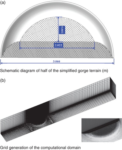
Table 1. Numerical conditions of the numerical model.

Parameters	Longitudinal (x)	Transverse (y)	Vertical (z)
Computational domain (m)	18.0	1.8	3.0
Grid number	116189 (in x-y plane)		50
Grid resolution (m)	0.005–0.45	0.005–0.08	0.001–0.43

2.3. Boundary conditions with a new form of turbulence kinetic energy profile

The inlet boundary conditions are very important parameters, and they should be as close to those of the wind tunnel tests or field measurements as possible in order to ensure the accuracy of the numerical results. However, achieving this is very difficult (Cao et al., 2012). Although there are many turbulence models for simulating different kinds of wind fields, the SST k-ω turbulence model has been more and more widely used in the numerical simulations of flow around bluff bodies due to its relatively high efficiency and accuracy (Aldas & Yapici, 2014; Casella, Langreder, Fischer, Ehlen, & Skoutelakos, 2014; W. Yang et al., 2008). When employing the SST k-ω turbulence model to simulate the wind field, the inlet boundary conditions are usually the profiles of mean wind speed U, turbulence kinetic energy k, and specific dissipation rate ω. Hu et al. (2013) proposed a set of inlet boundary conditions incorporating the profiles of U, k and ω based on previous research (Equations (1) to (3)), and used these inlet boundary conditions to simulate the mean wind speeds and turbulence intensities above a trapezoidal hill with high accuracy: (1) (2) (3) where z is the height from the ground, U(z), k(z), and ω(z) are the values of mean wind speed, turbulence kinetic energy, and specific dissipation rate at the height of z, respectively, z₀ is the aerodynamic roughness length, u_* is the friction velocity, κ is the von Kármán constant with κ ≈ 0.41, and C_u1 and C_u2 are two constants that can be determined by nonlinearly fitting the data from wind tunnel tests and field measurements (for further details, see Hu et al., 2013).

Generally speaking, the mean wind speed profile in the range of the ABL can be well described by the power law or log law (Simiu & Scanlan, 1996). However, the log law is more useful in the process of theoretical derivation (Richards & Hoxey, 1993), as shown in Equations (1) to (3). Figure 5 shows the mean wind speed profile presented in Figure 3(a) fitted by the log law using Equation (1). It can be seen that the fitting has a good accuracy because the value of Adj. R-Square (OriginLab Corporation 2010) is larger than 0.97. Therefore, Equation (1) and the fitting parameters can be directly adopted in the numerical simulation when using the SST k-ω turbulence model. The definition of the turbulence kinetic energy k includes two variables, i.e. the mean wind speed U and the turbulence intensity I, where the mean wind speed U increases and the turbulence intensity I decreases as the height increases. As a result, the curve of the turbulence kinetic energy profile is not smooth and usually has some turning points, as shown in Y. Yang, Gu, Chen, and Jin (2009), wherein the profile of the turbulence kinetic energy k first increases and then decreases as the height increases. Usually, the inlet turbulence kinetic energy k used in numerical simulations takes the form of Equation (4) (Blocken, Carmeliet, & Stathopoulos, 2007; Gao & Chow, 2005; Lakehal, 1998; Ramponi & Blocken, 2012): (4)

Figure 5. Mean wind speed profile and its fitted results by the log law.

where I_u(z) is the turbulence intensity and a_k is the turbulence kinetic energy coefficient that is a constant here (Hu et al., 2013; Ramponi & Blocken, 2012). Figure 6 shows the profile of k calculated by using Equation (4) (a_k = 1.0) according to the wind tunnel test data presented in Figure 3, where the curve of the k profile is also not smooth and cannot be fitted by Equation (2) with high accuracy. In this circumstance, in order to solve the fitting problem of k, the commonly used form of k in Equation (4) should be changed to (5)

Figure 6. Profile of k according to the wind tunnel test data.

where the value of a_k(z) can change with the height z. Therefore, a_k(z) is called the alterable turbulence kinetic energy coefficient here, but the value range of a_k(z) is still from 0.5 to 1.5 (Ramponi & Blocken, 2012). In this way, it is possible to take a small value of a_k(z) at a higher position and take a large value of a_k(z) at a lower position. Then the shape of the profile of k can change and can thus be fitted by Equation (2) with very high accuracy. Since the inlet profile of U in the numerical simulation can directly adopt the form of Equation (1), the changes of the inlet profile of k are equivalent to the changes of the inlet profile of I_u according to the relationship in Equation (5). Certainly, the effects of the changes of k (or I_u) at the inlet must be considered in the final results. However, such a practice must be validated before the actual numerical simulations are carried out.

To investigate the feasibility of the method of changing the values of k or I_u at the inlet, several sets of a_k(z) need to be given to simulate the wind field over the gorge terrain. On the one hand, the values of a_k(z) are in the range of 0.5 to 1.5; on the other hand, according to the wind tunnel tests by Cao and Tamura (2007), the inlet turbulence generally has a small effect on the mean wind speed distribution above the height not far from the surface of rough terrain on a hill. Furthermore, it is not difficult to understand that the turbulence intensities with certain distances above the simplified gorge terrain will generally depend on the inlet turbulence intensities, as the effects of the simplified gorge terrain can be ignored in this case. From the above observations, it can be concluded that changing the values of a_k(z) at the higher measurement positions will not significantly influence the final results of the mean wind speed and turbulence intensity at heights not far from the gorge terrain. Therefore, the values of a_k(z) at the highest measurement position are all determined to be 0.5. However, changing the values of a_k(z) at the lower measurement positions may influence the final results of the mean wind speed and turbulence intensity near the gorge terrain, and this issue needs to be confirmed by the actual numerical simulation practices. In such circumstances, three different values of a_k(z) at the lowest measurement position are chosen as 1.5, 1.25 and 1.0. Then, the three sets of inlet turbulence kinetic energy profiles denoted by k₁(z), k₂(z) and k₃(z), respectively can be determined by Equation (2) with these three pairs of fitted values (Figure 7). Therefore, the profiles of a_k(z) denoted by a_k1(z), a_k2(z) and a_k3(z) can also be determined by Equation (5) (Figure 8). In the numerical simulation, the profiles of inlet turbulence kinetic energy take the values of k₁(z), k₂(z) and k₃(z) and the profiles of the inlet specific dissipation rate ω₁(z), ω₂(z) and ω₃(z), respectively can also be determined by Equation (3). The three sets of inlet boundary conditions and parameters are listed in Table 2.

Figure 7. Three sets of turbulence kinetic energy profiles k₁, k₂ and k₃.

Figure 8. Three sets of turbulence kinetic energy coefficients a_k1, a_k2 and a_k3.

Table 2. Three sets of boundary conditions and parameters.

Boundaries	Boundary conditions and parameters
		U
		k
Inlet	Velocity inlet	ω
Outlet	Pressure-outlet	p = 0
Top/Side	Wall	Ks = 0
Symmetry side	Symmetry
Bottom	Wall	Ks = 0, Specify the value of τw

The top and the side of the computational domain are modeled as a smooth wall, while the symmetrical side is modeled as the symmetry boundary condition and the pressure-outlet boundary condition is applied at the outlet. At the bottom of the computational domain, a smooth wall is also modeled, but a certain wall shear stress must be specified to make the wall condition compatible with the inlet boundary conditions (Blocken, Stathopoulos, & Carmeliet, 2007). Furthermore, to ensure that the inlet boundary conditions satisfy the SST k-ω turbulence model, the source terms S_k and S_ω should be defined in the k and ω transport equations (Fluent, 2006), as shown in Equations (6) and (7). According to the research by Hu et al. (2013), the forms of S_k and S_ω can be derived as shown in Equations (8) and (9). It can be seen that there are four unknown coefficients C_1k, C_2k, C_1ω and C_4ω in Equations (8) and (9), and the values need to be obtained first. Fortunately, the values of C_1k, C_2k, C_1ω and C_4ω can be determined by modeling the equilibrium ABL in the empty computational domain (Hu et al., 2013), and the details will be discussed later. (6) (7) (8) (9) where S_k and S_ω are the source terms for the k and ω transport equations, respectively and C_1k, C_2k, C_1ω and C_4ω are the coefficients (for more details, see Fluent Inc., 2006; Hu et al., 2013).

The flow is supposed to be incompressible and steady. When choosing the discretization schemes for the governing equations, the SIMPLEC algorithm is applied to the pressure-velocity coupling, the second-order interpolation scheme is used for pressure, and the second-order upwind scheme is adopted for moment and turbulence properties. The values set for the inlet boundary are used to initialize the flow field, and the scaled residuals for all variables are set to be 10⁻⁶.

2.4. Modeling of the equilibrium ABL

Many researchers (Blocken, Carmeliet, & Stathopoulos, 2007; Blocken, Stathopoulos, & Carmeliet, 2007; Cao et al., 2012; Hu et al., 2013; W. Yang et al., 2008) have emphasized that an equilibrium ABL should be achieved in an empty computational domain before conducting the actual CFD numerical simulation, as this can greatly improve the accuracy of the results. Therefore, in this paper, an equilibrium ABL must be achieved in the empty computational domain first. To achieve this, the grid generation scheme, boundary conditions and parameters all are as close as possible to those of the actual numerical simulation of the simplified gorge terrain.

In this paper, the method proposed by Hu et al. (2013) is adopted for modelling the equilibrium ABL in the empty computational domain with the three sets of inlet boundary conditions listed in Table 2. According to this method, the profiles of U, k and ω at the inlet (x = −6 m) and at the model position (x = 0 m, defined as the center of the terrain model) can be obtained (Figure 9.) To better show the differences of the above parameters between these two positions, the relative errors of these parameters are also given. It can be seen that the profiles of U at the model position all agree very well with those at the inlet. However, there are some differences between the profiles of ω at these two positions. On the one hand, some differences of the values of ω have little influence on the values of U and I_u over the terrain (Hu et al., 2013). On the other hand, the wind characteristics near the ground are mainly focused on in wind engineering. For instance, for heights less than 0.5 m (or 300 m for the actual full-scale value), the relative errors of ω all become smaller, which is acceptable for the present study. Similarly, for heights less than 0.5 m, the average relative errors of k are all generally less than 6.0%, which is enough to meet the requirements of the study. From the above, it can be concluded that the equilibrium ABL is satisfactorily achieved for each inlet boundary condition in the empty computational domain. Accordingly, the values of the three sets of the coefficients C_1k, C_2k, C_1ω and C_4ω and the shear stress can be determined from the results of the equilibrium ABL (Table 3). Based on the above equilibrium ABL and the coefficients, the wind characteristics over an area of simplified gorge terrain will be studied in detail.

Figure 9. Profiles of U, k, and ω and relative errors at the inlet and at the model position for the three sets of inlet boundary conditions: (a) the first set, (b) the second set, and (c) the third set.

Table 3. Three sets of shear stresses and source terms.

Parameters	Values
Shear stresses
Source terms for k
Source terms for ω

2.5. Comparison of the numerical results and the test results

Once the equilibrium ABL is satisfactorily achieved for each inlet boundary condition in the empty computational domain, the actual numerical simulation on the wind characteristics over the area of simplified gorge terrain can be conducted. In the present study, the values of the mean wind speed U and the turbulence intensity I_u are investigated. From the discussion in section 2.3, the mean wind speed U can be directly obtained from the numerical simulation, but the values of the turbulence intensity I_u – as per Equation (5) – are comprehensively determined by the mean wind speed U, the turbulence kinetic energy k and a_k(z), whose values can also be directly obtained from the numerical simulation and Figure 8.

Figure 10 shows the profiles of the mean wind speed U and the turbulence intensity I_u at the gorge center under the three different inlet boundary conditions, and the corresponding wind tunnel test results are also given. It can be seen that the three set values of U and I_u obtained by the numerical simulation are generally in a good agreement with those obtained by the wind tunnel test. When the error of the numerical results is quantitatively analyzed, it is found that for the first set of inlet boundary conditions (listed in Table 2), the average and maximum relative errors of U are 1.85% and 3.20%, respectively, and the average and maximum relative errors of I_u are 3.86% and 8.84%, respectively. For the second set of inlet boundary conditions, the average and maximum relative errors of U are 1.64% and 4.04%, respectively, and the average and maximum relative errors of I_u are 4.75% and 9.44%, respectively. For the third set of inlet boundary conditions, the average and maximum relative errors of U are 2.20% and 7.15%, respectively, and the average and maximum relative errors of I_u are 5.90% and 12.69%, respectively. Therefore, when using the first set of inlet boundary conditions, the errors of U and I_u are smallest, and the results of U and I_u in this case can meet the accuracy requirements in the actual numerical simulations.

Figure 10. Comparison of numerical results of mean wind speed and turbulence intensity at the gorge center with the corresponding wind tunnel test results for the three sets of inlet boundary conditions: (a) the first set, (b) the second set, and (c) the third set.

From the above numerical simulation practices, it can be concluded that the values of the mean wind speeds over the simplified gorge terrain are almost unchanged with the inlet turbulence kinetic energy as defined by Equation (5). A similar phenomenon was also observed by Hu et al. (2013) when investigating the mean wind speeds over a trapezoidal hill. More importantly, the above numerical simulation practices also indicate that the values of turbulence kinetic energy over the gorge terrain synchronously change with the inlet turbulence kinetic energy. Therefore, the values of the turbulence intensity over the gorge terrain determined by Equation (5) are almost the same when different inlet boundary conditions are adopted. However, it should be pointed out that the values of the inlet turbulence kinetic energy change around their corresponding test values, i.e., the values of the alterable turbulence kinetic energy coefficient a_k(z) are in the range of 0.5 to 1.5. Furthermore, the present wind characteristics over the gorge terrain are obtained with the oncoming wind flowing along the axis of the gorge terrain, which makes the terrain model a kind of streamline body and the flow separation not obvious under these circumstances. As a result, the wind field over the gorge terrain is simple and can be synchronously changed with the three different inlet boundary conditions. The above features may be the main reason for the effectiveness of the alterable turbulence kinetic energy coefficient method that is presented in Equation (5).

3. Simulations of the wind characteristics over simplified gorge terrain

To make the wind characteristics over the simplified gorge terrain more realistic and accurate, it is necessary to investigate them while varying parameters such as the included angle and the terrain height (Figure 1). Therefore, based on the area of simplified gorge terrain with an included angle of 120° and a terrain height of 0.25 m, another five areas of simplified gorge terrain were modeled in the computational domain. For three areas, the terrain height was kept constant at 0.25 m and the included angle set to 80°, 100° and 140°, then for the other two areas, the included angle was kept constant at 120° and the terrain height set to 0.20 m and 0.30 m. As such, the blockage ratios of the above five areas are about 5.9%, 5.7%, 4.8%, 4.6% and 6.1%, respectively, compared to about 5.4% for the default area with an included angle of 120° and a terrain height of 0.25 m. Therefore, the difference in the blockage ratios among all six areas of simplified gorge terrain is very small and could not have a significant effect on the wind characteristics. The first set of inlet boundary conditions, as the set with the highest accuracy, was used to model the wind characteristics over the areas of simplified gorge terrain with different included angles and terrain heights. Similarly, other conditions such as the grid generation scheme, boundary conditions and parameters were all kept as close as possible to those of the numerical simulation over the area of simplified gorge terrain with an included angle of 120° and a terrain height of 0.25 m.

3.1. Wind characteristics over simplified gorge terrain with different included angles

Figures 11 and 12 show the profiles of the mean wind speed U and turbulence intensity I_u at the center of the simplified gorge terrain with different included angles. The profiles of the mean wind speed and turbulence intensity at the inlet are also given for comparison. It can be seen from Figure 11 that the mean wind speed generally increases at the gorge center for the different included angles, and that the larger the included angle, the greater the increase of the mean wind speed at the gorge center. However, as the distance from the ground increases, the increase of the mean wind speed at the gorge center gradually levels off and becomes almost the same, regardless of the included angle. The main reason for this is that the gorge terrain has a small effect on the wind field that is far from the terrain model, i.e., the wind field far from the ground mainly depends on the wind field at the inlet. Furthermore, note that the mean wind speeds at the highest measurement position with the different included angles are almost equal, which indicates that the differences in blockage ratios among the above areas of simplified gorge terrain indeed have a very small influence on the wind field over the terrain.

Figure 11. Mean wind speed profiles at the gorge center for different included angles.

Figure 12. Turbulence intensity profiles at the gorge center for different included angles.

The values of the turbulence intensity at the gorge center with different included angles are much smaller than those at the inlet. As the included angles decrease, the values of the turbulence intensity tend to increase, but the tendency is small (Figure 12). Figure 13 shows the mean square deviation σ values of the turbulent flow at the gorge center and the inlet. It can be seen that the values of mean square deviation at the gorge center are much smaller than those at the inlet. Furthermore, the smaller the included angle is, the smaller the values of mean square deviation at the gorge center become. Generally, the above phenomena imply that the influences of the gorge terrain on the wind field in the gorge become larger when the included angles of the gorge terrain become smaller.

Figure 13. Mean square deviation profiles of the turbulent flow at the gorge center for different included angles.

3.2. Wind characteristics over simplified gorge terrain with different terrain heights

Figures 14 and 15 show the profiles of the mean wind speed U and turbulence intensity I_u at the center of the areas of simplified gorge terrain with different terrain heights and at the inlets. It can be seen that the mean wind speeds at the gorge centers are all larger than those at the inlet, but the turbulence intensities at the gorge centers are all smaller than those at the inlet. Furthermore, as the terrain height increases, the mean wind speed at the gorge center increases and the turbulence intensity at the gorge center decreases. However, the variation of the mean wind speed and turbulence intensity at the gorge center for different terrain heights is quite small. For instance, the maximum relative change ratios of the mean wind speeds at the gorge center with terrain heights of 0.20 m and 0.30 m compared to those with the terrain height of 0.25 m are only 1.4% and 1.3%, respectively. For the different included angles as discussed in section 3.1, the maximum relative change ratios of the mean wind speeds at the gorge center with the included angles of 80°, 100° and 140° compared to those with the included angle of 120° are all larger than 5.0%. As mentioned earlier, the maximum and minimum blockage ratios of the areas of gorge terrain with different terrain heights are 6.1% and 4.6%, respectively. In comparison, the maximum and minimum blockage ratios of the areas of gorge terrain with different included angles are 5.9% and 4.8%, respectively. Therefore, the differences in mean wind speed at the gorge center with different terrain heights are probably caused by the differences in the blockage ratios. On the other hand, it is not difficult to understand that as the terrain height increases, the influence of the side slopes of the gorge terrain on the wind characteristics at the gorge center decreases, especially for the measurement positions far from the ground due to their distances far from the side slopes of the gorge too. From the above, it can be concluded that the effect of the terrain height on the wind characteristics at the gorge center is very small, and the differences in mean wind speed and turbulence intensity shown in Figures 14 and 15 can be regarded as being caused by the differences in the blockage ratios. However, the differences in the blockage ratios do not need to be considered when investigating the wind characteristics at the gorge center with different included angles, as the effect of blockage ratio is so small compared to the effect of the included angle.

Figure 14. Mean wind speed profiles at the gorge center for different terrain heights.

Figure 15. Turbulence intensity profiles at the gorge center for different terrain heights.

4. Conclusions

To obtain some basic information that could potentially inform on the general evaluation of effects introduced by gorge terrain, an area of V-shaped simplified gorge terrain was adopted in the present study. Based on the SST k-ω turbulence model, the wind characteristics – including the mean wind speed and turbulence intensity – at the center of the area of simplified gorge terrain was investigated for different included angles and terrain heights. The main conclusions are summarized as follows:

1. To ensure that the profile of turbulence kinetic energy at the inlet boundary of the computational domain had the same values as those of the wind tunnel test, a new form of turbulence kinetic energy profile was defined. Based on the achieved equilibrium ABL, the average relative error of the mean wind speed at the gorge center for three different inlet boundary conditions was found to be 1.85%, 1.64% and 2.20%, and the average relative error of the turbulence intensities was found to be 3.86%, 4.75% and 5.90%, respectively. These errors indicate that the above numerical results are generally in good agreement with those obtained from the wind tunnel test. Also, it is proved that the new form of turbulence kinetic energy profile with an alterable coefficient (Equation (5)) is effective and practical for simulating the wind characteristics over the simplified gorge terrain.

2. For the areas of gorge terrain with different included angles, the mean wind speed generally increases at the gorge center compared with the mean wind speed at the inlet, and the larger the included angle, the more significant the increase in the mean wind speed at the gorge center. The turbulence intensity at the gorge center with different included angles is much smaller than that the at inlet, and with as included angle decreases, the turbulence intensity increases, but the tendency is small.

3. The mean square deviation values of the turbulent flow at the gorge center are much smaller than those at the inlet, and the smaller the included angle is, the smaller the values of the mean square deviation at the gorge center become.

4. The effect of the terrain height on the mean wind speed and turbulence intensity at the gorge center is very small.

While the present study has made some progress in terms of understanding the wind characteristics over gorge and valley terrains, it is also important to highlight the limitations of this study:

1. The numerical results – including the mean wind speeds and turbulence intensities – in this paper are obtained based on the solution of a steady RANS method (SST k-ω turbulence model). Although the computational time can be greatly reduced, the time-history of the wind speed cannot be obtained. Therefore, the values of the wind power spectra in the gorge terrain cannot be directly investigated in the present study.

2. The cross-sections of simplified gorge terrains in this paper are all shaped as a ‘V’, but some gorge terrains will be differently shaped. Therefore, the gorge terrains with other typical shapes need to be further studied.

Overcoming these limitations will be the focus of future work.

Disclosure statement

No potential conflict of interest was reported by the authors.

Additional information

Funding

This work was supported by the National Natural Science Foundation of China [grant numbers 51408496 and 90915006], and the National Basic Research Program of China [grant numbers 2015CB057706 and 2015CB057701.

References

- Aldas, K., & Yapici, R. (2014). Investigation of effects of scale and surface roughness on efficiency of water jet pumps using CFD. Engineering Applications of Computational Fluid Mechanics, 8(1), 14–25. doi: 10.1080/19942060.2014.11015494
- Blocken, B., Carmeliet, J., & Stathopoulos, T. (2007). CFD evaluation of wind speed conditions in passages between parallel buildings—Effect of wall-function roughness modifications for the atmospheric boundary layer flow. Journal of Wind Engineering and Industrial Aerodynamics, 95(9–11), 941–962. doi: 10.1016/j.jweia.2007.01.013
- Blocken, B., Stathopoulos, T., & Carmeliet, J. (2007). CFD simulation of the atmospheric boundary layer: Wall function problems. Atmospheric Environment, 41(2), 238–252. doi: 10.1016/j.atmosenv.2006.08.019
- Bullard, J. E., Wiggs, G. F. S., & Nash, D. J. (2000). Experimental study of wind directional variability in the vicinity of a model valley. Geomorphology, 35(1–2), 127–143. doi: 10.1016/S0169-555X(00)00033-7
- Cao, S., & Tamura, T. (2006). Experimental study on roughness effects on turbulent boundary layer flow over a two-dimensional. Journal of Wind Engineering and Industrial Aerodynamic, 94(1), 1–19. doi: 10.1016/j.jweia.2005.10.001
- Cao, S., & Tamura, T. (2007). Effects of roughness blocks on atmospheric boundary layer flow over a two-dimensional low hill with/without sudden roughness change. Journal of Wind Engineering and Industrial Aerodynamics, 95, 679–695. doi: 10.1016/j.jweia.2007.01.002
- Cao, S., Wang, T., Ge, Y., & Tamura, Y. (2012). Numerical study on turbulent boundary layers over two-dimensional hills-effects of surface roughness and slope. Journal of Wind Engineering and Industrial Aerodynamic, 104–106, 342–349. doi: 10.1016/j.jweia.2012.02.022
- Casella, L., Langreder, W., Fischer, A., Ehlen, M., & Skoutelakos, D. (2014). Dynamic flow analysis using an OpenFOAM based CFD tool: Validation of turbulence intensity in a testing site. ITM Web of Conferences 2, 1–12.
- CCCC Highway Consultants. (2004). Wind-resistent design specification for highway bridges. Commendatory trade standards of the People’s Republic of China, Beijing. (in Chinese)
- Derickson, R. G., & Peterka, J. A. (2004). Development of a powerful hybrid tool for evaluating wind power in complex terrain: atmospheric numerical models and wind tunnels. 42nd AIAA Aerospace Sciences Meeting and Exhibit. 5–8 January 2004, Reno, USA.
- Fluent. (2006). Fluent 6.3 user’s guide. Lebanon, New Hampshire: Fluent Inc.
- Gao, Y., & Chow, W. K. (2005). Numerical studies on air flow around a cube. Journal of Wind Engineering and Industrial Aerodynamics, 93(2), 115–135. doi: 10.1016/j.jweia.2004.11.001
- Hu, P., Li, Y. L., Cai, C. S., Liao, H. L., & Xu, G. J. (2013). Numerical simulation of the neutral equilibrium atmospheric boundary layer using the SST k-omega turbulence model. Wind and Structures, 17(1), 87–105. doi: 10.12989/was.2013.17.1.087
- Hu, P., Li, Y. L., Huang, G. Q., Kang, R., & Liao, H. L. (2015). The appropriate shape of the boundary transition section for a mountain-gorge terrain model in a wind tunnel test. Wind and Structures, 20(1), 15–36. doi: 10.12989/was.2015.20.1.015
- Iizuka, S., & Kondo, H. (2004). Performance of various sub-grid scale models in large-eddy simulations of turbulent flow over complex terrain. Atmospheric Environment, 38, 7083–7091. doi: 10.1016/j.atmosenv.2003.12.050
- Iizuka, S., & Kondo, H. (2006). Large-eddy simulations of turbulent flow over complex terrain using modified static eddy viscosity models. Atmospheric Environment, 40, 925–935. doi: 10.1016/j.atmosenv.2005.10.014
- Kim, H. G., Patel, V. C., & Lee, C. M. (2000). Numerical simulation of wind flow over hilly terrain. Journal of Wind Engineering and Industrial Aerodynamic, 87(1), 45–60. doi: 10.1016/S0167-6105(00)00014-3
- Lakehal, D. (1998). Application of the k-ε model to flow over a building placed in different roughness sublayers. Journal of Wind Engineering and Industrial Aerodynamics, 73(1), 59–77. doi: 10.1016/S0167-6105(97)00279-1
- Li, C. G., Chen, Z. Q., Zhang, Z. T., & Cheung, J. C. K. (2010). Wind tunnel modeling of flow over mountainous valley terrain. Wind and Structures, 13(3), 275–292. doi: 10.12989/was.2010.13.3.275
- Liu, Z. (2012). Investigation of flow characteristics around square cylinder with inflow turbulence. Engineering Applications of Computational Fluid Mechanics, 6(3), 426–446. doi: 10.1080/19942060.2012.11015433
- Li, Y. L., Hu, P., Cai, X. T., Tang, K., & Liao, H. L. (2011). Spatial distribution feature of wind fields over bridge site with a deep-cutting gorge by numerical simulation method. The 13th International Conference on Wind Engineering. 10–15 July 2011, Amsterdam, Netherlands.
- Maurizi, A., Palma, J. M. L. M., & Castro, F. A. (1998). Numerical simulation of the atmospheric flow in a mountainous region of the North of Portugal. Journal of Wind Engineering and Industrial Aerodynamics, 74–76, 219–228. doi: 10.1016/S0167-6105(98)00019-1
- Miller, C. A., & Davenport, A. G. (1998). Guidelines for the calculation of wind speed-ups in complex terrain. Journal of Wind Engineering and Industrial Aerodynamics, 74–76, 189–197. doi: 10.1016/S0167-6105(98)00016-6
- OriginLab Corporation. (2010). Origin reference for origin 8.5 SR1. Northampton, Massachusetts, USA.
- Ramponi, R., & Blocken, B. (2012). CFD simulation of cross-ventilation for a generic isolated building: Impact of computational parameters. Building and Environment, 53, 34–48. doi: 10.1016/j.buildenv.2012.01.004
- Richards, P. J., & Hoxey, R. P. (1993). Appropriate boundary conditions for computational wind engineering models using the k-ε turbulence model. Journal of Wind Engineering and Industrial Aerodynamics, 46–47, 145–153. doi: 10.1016/0167-6105(93)90124-7
- Sierputowskia, P., Ostrowskia, J., & Cenedeseb, A. (1995). Experimental study of wind flow over the model of a valley. Journal of Wind Engineering and Industrial Aerodynamics, 57(2–3), 127–136. doi: 10.1016/0167-6105(95)00009-G
- Simiu, E., & Scanlan, R. H. (1996). Wind effects on structures: Fundamentals and applications to design (3th ed.). New York, USA: Wiley.
- Tamura, T., Okuno, A., & Sugio, Y. (2007). LES analysis of turbulent boundary layer over 3D steep hill covered with vegetation. Journal of Wind Engineering and Industrial Aerodynamic, 95(9–11), 1463–1475. doi: 10.1016/j.jweia.2007.02.014
- Uchida, T., & Ohya, Y. (2003). Large-eddy simulation of turbulent airflow over complex terrain. Journal of Wind Engineering and Industrial Aerodynamics, 91(1–2), 219–229. doi: 10.1016/S0167-6105(02)00347-1
- Wan, F., Porté-Agel, F., & Stoll, R. (2007). Evaluation of dynamic subgrid-scale models in large-eddy simulations of neutral turbulent flow over a two-dimensional sinusoidal hill. Atmospheric Environment, 41, 2719–2728. doi: 10.1016/j.atmosenv.2006.11.054
- Yang, W., Quan, Y., Jin, X., Tamura, Y., & Gu, M. (2008). Influences of equilibrium atmosphere boundary layer and turbulence parameter on wind loads of low-rise building. Journal of Wind Engineering and Industrial Aerodynamics, 96(10–11), 2080–2092. doi: 10.1016/j.jweia.2008.02.014
- Yang, Y., Gu, M., Chen, S., & Jin, X. (2009). New inflow boundary conditions for modelling the neutral equilibrium atmospheric boundary layer in computational wind engineering. Journal of Wind Engineering and Industrial Aerodynamics, 97(2), 88–95. doi: 10.1016/j.jweia.2008.12.001
- Zheng, D. Q., Zhang, A. S., & Gu, M. (2012). Improvement of inflow boundary condition in large eddy simulation of flow around tall building. Engineering Applications of Computational Fluid Mechanics, 6(4), 633–647. doi: 10.1080/19942060.2012.11015448
- Zhu, L. D., Ren, P. J., Chen, W., Zhou, C., & Wang, J. Q. (2011). Investigation on wind profiles in the deep gorge at the Balinghe bridge site via field measurement. Journal of Experiments in Fluid Mechanic, 25(4), 15–21. (in Chinese)