Evaluation of near-wall solution approaches for large-eddy simulations of flow in a centrifugal pump impeller

ABSTRACT

The turbulent flow in a centrifugal pump impeller is bounded by complex surfaces, including blades, a hub and a shroud. The primary challenge of the flow simulation arises from the generation of a boundary layer between the surface of the impeller and the moving fluid. The principal objective is to evaluate the near-wall solution approaches that are typically used to deal with the flow in the boundary layer for the large-eddy simulation (LES) of a centrifugal pump impeller. Three near-wall solution approaches –the wall-function approach, the wall-resolved approach and the hybrid Reynolds averaged Navier–Stoke (RANS) and LES approach – are tested. The simulation results are compared with experimental results conducted through particle imaging velocimetry (PIV) and laser Doppler velocimetry (LDV). It is found that the wall-function approach is more sparing of computational resources, while the other two approaches have the important advantage of providing highly accurate boundary layer flow prediction. The hybrid RANS/LES approach is suitable for predicting steady-flow features, such as time-averaged velocities and hydraulic losses. Despite the fact that the wall-resolved approach is expensive in terms of computing resources, it exhibits a strong ability to capture a small-scale vortex and predict instantaneous velocity in the near-wall region in the impeller. The wall-resolved approach is thus recommended for the transient simulation of flows in centrifugal pump impellers.

KEYWORDS:

• large-eddy simulation
• near-wall solution
• evaluation
• centrifugal pump impeller

1. Introduction

The large-eddy simulation (LES) has the advantage of using less complex calculations compared to direct numerical simulation (DNS), while still achieving high accuracy. The LES solution captures the random character of an unsteady flow field and produces a closer agreement with actual measurements than the Reynolds averaged Navier–Stoke (RANS) method. LES is showing great potential for capturing the unsteady behavior of a vortex in a separating and rotating flow, such as the flow in a centrifugal pump impeller (Breuer, Jovicic, & Mazaev, 2003).

LES is designed to explicitly compute the geometry-dependent and grid-scale flows, and to model small-scale turbulence using subgrid-scale (SGS) models. Wall modeling was first used in LES a number of decades ago (Deardorff, 1970; Schumann, 1975). The anisotropic modes of turbulence (Jimenez & Moser, 2000) are not accurately modeled by most SGS models and, near to the wall, the number of these modes’ scales is proportionate to (Baggett, Jimenez, & Kravchenko, 1997). The requirements of near-wall solutions for LES are nearly as high as those of DNS, which restricts the applicability of the LES method in flows with high Reynolds numbers and complex geometries. In order to mitigate this restriction, many researchers have made great efforts to develop wall treatments for LES (Cabot & Moin, 2000; Piomelli & Balaras, 2002).

The widely adopted approach in the near-wall region’s treatment is the wall-function approach (Wang, 2004). An algebraic relationship between the local wall stresses and the tangential velocities is provided by this approach at the first off-wall velocity nodes. The resource requirements of LES for high Reynolds number near-wall flows are reduced tremendously by using the wall-function approach, while the effects of near-wall processes on the outer flow are still described realistically. Several methods have been proposed since the first computations of Deardorff (1970), which assumed a profile for the transient flow velocity between the nodes that are closest to the wall and the wall itself. The log-law profile (Schumann, 1975) and the th power-law profile (Werner & Wengle, 1993) have been widely used in the channel flow on rather coarse grids, and both profiles are designed to predict the instantaneous wall shear stress at the node nearest to the wall for a given velocity condition. Piomelli (2008) pointed out that making improvements in logarithmic law could potentially clarify many non-equilibrium effects, but that logarithmic law cannot accurately calculate skin-friction values in separated flows. However, the effectiveness of this technique has not been validated in the separated flow in an impeller channel.

Another approach used in the treatment of a near-wall region is the wall-resolved approach (Wang & Moin, 2000), which solves the flow in the near-wall region directly. It is similar to DNS, but without requiring further modeling. An extremely fine grid is required by this approach. The viscous sublayer is resolved, which is down to a wall-normal distance of y⁺= ○(1), with high streamwise and spanwise solutions (x⁺ = ○(50), z⁺ = ○(10)). This approach can successfully predict the flow structure in the near-wall region when the viscous effect in the near-wall region is weak, and a relatively coarse grid can be adopted to satisfactorily resolve the spatial scales. The vortex shedding behind blunt bodies in a free stream flow (Krajnovic & Davidson, 2002; Rodi, 1998) or the jets in a cross flow (Jones & Wille, 1996) are the typical cases mentioned above. In such situations, the non-dissipative processes appearing at the SGS level are ignorable. The numerical errors are relatively low in number, which are affiliated with the resolution of the influential scales. However, the viscous effect in the near-wall region is influential in many practically important flows, such as the flow in an impeller channel. In such circumstances, viscous near-wall processes have strong influences on the primary flow’s properties, presenting the LES method with a much greater challenge. Two research groups simulated the separated flow within an asymmetric plane diffuser with moderate Reynolds numbers (Herbst, Schlatter, & Henningson, 2007; Wu, Schluter, & Moin, 2006). Wu et al. (2006) used two meshes (a fine mesh of 590 × 100 × 110 and a coarse mesh of 360 × 80 × 80) and ensured that the first layer of the cell centers was located below the viscous sublayer, while the spanwise direction was treated homogeneously.

The third approach is the hybrid RANS/LES method, which parameterizes all the scales of vortices in the near-wall region with the RANS model and simulates the fully developed turbulent flow with LES. When setting up the hybrid RANS/LES, three main design aspects should be determined, starting with which turbulence models should be employed in the RANS and LES regions. Tucker (2003) and Tucker and Davidson (2004) used one-equation models in both regions. It should be noted that the modified one-equation Spalart–Allmaras RANS model (Spalart & Allmaras, 1992) is the most widely-used turbulence model (Nikitin, Nicoud, Wasistho, Squires, & Spalart, 2000; Spalart, 2000). Some researchers used two-equation models in RANS regions such as or in order to construct the hybrid RANS/LES model (Dejoan & Schiestel, 2001; Menter, Kuntz, & Langtry, 2003). An explicit algebraic Reynolds stress model was employed in the RANS region in Jaffrezic and Breuer (2008). The second aspect concerns how the LES–RANS interface is defined. Davidson and Peng (2003) and Hamba (2003) chose a selected grid plane as the LES–RANS interface. Much work has been carried out in automatically defining the interface (Davidson & Dahlstrom, 2005; Spalart, 2000; Temmerman, Hadziabdicb, & Leschzinera, 2005), and it can be seen that automatic definition has an advantage over fitting the interface.

The third aspect concerns how to couple the two regions. The resolved turbulence of the LES region is accurate enough to be applied to the RANS region, but the resolved turbulence of the RANS region does not have the level of accuracy needed to trigger the LES equations to correctly resolve the turbulence, and has unreasonable turbulent characteristics. Many researchers have made great efforts to resolve this deficiency. To reduce the high jump of the shear stress across the interface, Temmerman, Leschziner, and Hanjalic (2002) recommended suppressing the modeled stresses for the Unsteady Reynolds Averaged Navier Stokes region. Piomelli, Balaras, and Pasinato (2003) suggested a backscatter in the interface region for generating resolved fluctuations. Davidson and Billson (2006) proposed adding fluctuations that were taken from synthesized homogeneous turbulence to the momentum equations at the RANS/LES interface. Some methods have been used for accelerating the reproduction of momentum-transporting eddies near the interface region, but none of them have the necessary robustness to make the method widely applicable. In the hybrid RANS/LES approach, the RANS model is employed to parameterize all scale vortices in the near-wall region. The interface can be artificially introduced and the variables couple between the RANS and LES regions. However, all of the above may introduce a new source of error; therefore, the precision of the technique has to be verified in separated flows, such as the flow in an impeller channel.

Su, Li, Li, Wei, and Zhao (2012) performed a simulation of complex three-dimensional flows in turbo-machines with both LES and RANS methods using the same the meshing system. It was found that the LES method coupled with the Smagorinsky–Lilly model can predict the running efficiency much better than the RANS method with a standard model. However, the detail of the near-wall solution approach was not discussed. The wall function and the near-wall models for modeling the near-wall region were tested by Galván, Reggio, and Guibault (2011), who also evaluated the accuracy of turbulence models for the swirling flow in a turbine draft tube. Significant differences were exhibited in the results due to the use of two near-wall solution approaches using the y⁺1 grid. An alternative hybrid RANS/LES strategy was used by Mockett, Fuchs, and Thiele (2012). The near-wall RANS modeling removed the Reynolds number scaling of the tangential grid spacing and the resolved turbulent fluctuations in the outer boundary layer were sustained by the LES. Golshan, Tejada-Martínez, Juha, and Bazilevs (2015) employed the LES method with near-wall modeling. In their method, the core flow was reasonably well resolved and the unresolved near-wall region was modeled through suitable boundary conditions, which obviated the need to use small time steps and fine meshes in the near-wall region.

The flow in a centrifugal pump impeller has the following characteristics: complex wall-bounded conditions, vortices shedding behind bluff bodies (blades) in the flow, an adverse pressure gradient resulting from a diffuse flow in the passage, and flow separation at the near-wall region. The effects of an anisotropic flow caused by strong rotating and high-curvature passages are significant, and must be taken into account. The factors mentioned above present a challenge to implementing LES for centrifugal pump impellers. Although many studies have been performed for the solution methods in the near-wall region, it is still unknown which solution method is most effective for simulating the flow in the centrifugal pump impeller. In view of the advantage of LES in simulating turbulence fluctuations in complex flows, it is necessary to evaluate the various methods for modeling the near-wall region by simulating the flows inside the centrifugal pump impeller.

This paper evaluates three approaches: the wall-function approach, the wall-resolved approach and the hybrid RANS/LES approach, all of which are used in a shrouded six-bladed centrifugal pump impeller. The simulation was carried out by Fluent (Ansys Inc., 2009). The following section describes the formulation of the SGS model and the approaches to the near-wall region used in the paper. After this, the parameters of the pump and the computational conditions are given. Next, the results of time-averaged and instantaneous velocities and the turbulent kinetic energy predicted by the three approaches are analyzed, and the data are compared with previous experimental results obtained from particle imaging velocimetry (PIV) and laser Doppler velocimetry (LDV) measurements. The conclusions are then presented in the final section.

2. Mathematical modeling

2.1. Governing equations

LES governing equations can be expressed by applying a filter to the continuity equation and the Navier–Stokes equations, described here in an incompressible form (Germano, Piomelli, & Moin, 1991), and also available in Yang, Wang, and Zhou (2012): (1) (2) where the overbar represents spatial filtering, is the density, is the kinematic viscosity, represents the resolved velocity components, is the resolved pressure, represents the source terms and represents the SGS stress tensor, which is defined by .

LES governing equations have an additional SGS stress tensor compared with the original Navier–Stokes governing equations. The additional SGS stress tensor is a second-order symmetrical tensor that includes six independent variables, and is modeled using the SGS model to close the equations.

2.2. SGS modeling

The SGS model is used to close Equations (1) and (2). The dynamic Smagorinsky model (DSM; Germano et al., 1991) is adopted as the SGS model in this study. The DSM is an eddy-viscosity model based on Boussinesq’s hypothesis (see Yang et al., 2012). According to Yang et al. (2012), the DSM is better suited to predicting a complex flow in a centrifugal pump impeller than the Smagorinsky model (SM). By the comprehensive consideration of its computational efficiency and accuracy, the DSM was finally employed. The DSM computes SGS stress as (3) where is the resolved strain-rate tensor and is the SGS stress viscosity, which is defined as (4) where represents the magnitude of the resolved strain-rate tensor, C_s is the non-dimensional model coefficient and is the filtered scale.

In the DSM, based on the Germano identity and the scale invariance assumption, C_s is computed at every time step and position in the flow. The Germano identity is defined as (5) where represents the stress on a test filter scale , and represents the resolved tress tensor, which can be calculated by the resolved scales.

Applying Equation (3) in order to model the SGS stress on a test filter scale, can be expressed as (6)

Substituting Equations (3) and (6) into Equation (5), and considering the scale invariance assumption, the result is (7)

Let (8) then Equation (7) can be expressed as (9)

Lilly (1992) suggests using the least squares minimization of the error to calculate the value of C_s: (10)

2.3. Solution approaches for the near-wall region

2.3.1. Wall-resolved approach

In the wall-resolved approach, the LES models are employed both inside and outside the boundary layer. Under such circumstances there are two issues to be considered in the computational process. First, a fine enough grid is required in order to resolve the small-sized eddies in the near-wall region. Second, the matter of how to resolve the viscous sublayer and buffer regions in which the flow is almost laminar needs to be addressed. In this work, a fine grid that fulfills the requirements of resolving the viscous sublayer down to a wall-normal distance y⁺ = ◯(1) and providing streamwise and spanwise resolutions (x⁺ = ◯(50), z⁺ = ◯(10), respectively) is used in the calculation for a wall-resolved approach. Because the DSM is adopted, by which means the model coefficient is adjusted automatically in order to satisfy the asymptotic behavior near to the wall, extra modeling is not required in the computation process.

2.3.2. Hybrid RANS/LES approach

In the hybrid RANS/LES approach, the unsteady RANS models are used in the boundary layer regions, and the LES models are employed in the separated regions. In the present study, the one-equation Spalart–Allmaras model (Spalart, 2000) was applied in the RANS regions and the DSM was employed in the LES regions.

In the Spalart–Allmaras model, the transport equation is given as (11) where Y is the destruction of turbulent viscosity that appears in the near-wall region because of wall blocking and viscous damping, G is the production of turbulent viscosity, and and are the constants.

2.3.3. Wall-function approach

The wall-function approach is a set of semi-empirical formulas establishing a linkage between the solution variables in the near-wall cells and the corresponding values on the wall. A wall-function approach needs the instantaneous wall shear stress corresponding to the instantaneous velocity at the first cell. The generally existing formulations are formed based on a composite relation between u⁺ and y⁺, which is applicable across the whole near-wall layer. In the present study, the wall-function approach suggested by Kader (1981) is adopted. It is expressed as follows: (12) where , , is the friction velocity defined as , is the distance of this point from the wall, is the Von Kármán constant, E = 9.793 and .

3. Numerical modeling

3.1. Parameters of the pump impeller

The investigated impeller is a shrouded centrifugal impeller (Figure 1). In the design condition, the pump flow rate is Q_d = 3.06 l/s and the head is H_d = 1.75 m for a single stage. Simulation of the design condition Q = Q_d is performed. The main geometrical data of the impeller and the normal operating conditions are both summarized in Table 1. This impeller was designed and tested by Pedersen, Larsen, and Jacobsen (2003).

Figure 1. The rotating part of the pump.

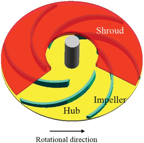
Table 1. Impeller geometry parameters and operating conditions.

Geometry	Symbol	Value	Unit
Inlet diameter	D1	71.0	mm
Outlet diameter	D2	190.0	mm
Blade thickness	t	3.0	mm
Number of blades	Z	6	-
Blade curvature radius		70.0	mm
Inlet angle		19.7	°
Outlet angle		18.4	°
Specific speed		26.3	-
Flow rate	Q	3.06	l/s
Flow rate coefficient		0.123	-
Head	H	1.75	m
Head coefficient		0.33	-
Rotational speed	n	725	rpm
Reynolds number	Re	1.4 × 10^6	-

3.2. Computational domain and mesh schemes

The computational domain only includes the impeller’s flow passage, which is verified in Yang et al. (2012). In order to minimize computer resources and take advantage of the geometrical symmetry of the impeller, only one passage was chosen, with the blade in the middle of the single flow passage. To reduce the boundary’s influence, extensions were made at the inlet and outlet of the flow passage (Figure 2).

Figure 2. (a) Computational domain of the impeller, (b) mesh for the wall-resolved approach, (c) mesh the for hybrid RANS/LES approach, and (d) mesh for the wall-function approach.

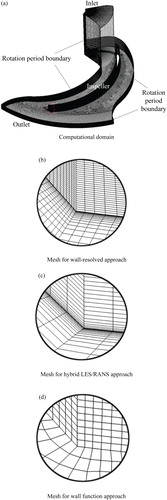
Due to the complexity of the computational domains, an unstructured hexahedron mesh was adopted because of its fine adaptability. In the near-wall region, a fine mesh is required for LES, so the mesh near to the wall is refined. Before the simulation results can be meaningfully discussed, two kinds of convergence should be considered at the first step: the convergence of the simulation results and the grid convergence. The mesh independence check is carefully carried out for the each approach before analyzing the simulation results. For the each simulation, the following was ensured: the residual root mean square (RMS) error converged to 10⁻⁴, the monitor points for pressures of interest were repeatable, and the domain imbalance was far below 1%. Finally, three different meshes are used in order to satisfy the grid requirements for the three near-wall solution approaches. In the wall-resolved approach simulation, the grid’s stretching factor is utilized in order to allow the wall-adjacent cells to be located 5 µm from the surface, corresponding to y⁺ values of less than 3 near the wall, whilst also refining the grids in both the streamwise and spanwise directions. A mesh with a total of 1,150,000 cells is utilized as the best compromise between solution-accuracy requirements and computational resources. In order to lay the wall-adjacent cells in log-law layers in the wall-function approach simulation, the wall-adjacent cells are located at 100  away from the wall, corresponding to y⁺ values located between 10 and 100 and a mesh with a total of 120,000 cells is utilized. In the hybrid RANS/LES approach simulation, the grids in the wall-normal direction are refined and the wall-adjacent cells are located 10 µm away from the wall, corresponding to y⁺ values of less than 5 and a mesh with a total of 220,000 cells. Figure 2 represents the mesh construction of the single flow passage.

3.3. Boundary conditions and numerical methods

A rotation reference frame is set for the flow passage with a rotating speed of the reference frame equal to the rotating speed of the impeller. A velocity inlet boundary condition is employed for the simulation. The value of the inlet velocity could be determined by the flow rate, including some fluctuation components that are estimated based on turbulent intensity I and turbulent length scale l. The turbulent intensity can be defined by the RMS of the velocity fluctuations, , divided by the mean free stream velocity, . It can be calculated as , and the value is 4%. The turbulence length scale, l, is a physical quantity that represents the size of the large eddies in the turbulent flow. The empirical relationship between the physical size of the characteristic length, L, and the size of the eddy, l, can be expressed as l = 0.007L, which can be used to get an approximate length scale (Mathey, Cokljat, Bertoglio, & Sergent, 2003). The estimated value in the present simulation is 0.00497 m. The velocity is normal for the inlet boundary. The Neumann condition, , is considered for the pressure. On the outlet of the passage, the value of the pressure is given, and the Neumann condition is considered for the velocity. A rotation period boundary condition is set for the right and left sides of the passage. A non-slip wall condition is considered, as u = 0, v = 0, w = 0. The Semi Implicit Method for Pressure Linked Equations method is used to solve pressure-velocity coupling. The second-order time scheme is used in the discrete time domain. The time step is set to 0.001 s. The lift force of the blade is monitored and the statistical averaging starts when the lift force is stabilized. More than 3000 time step results are used to generate the statistics. The simulations were carried out on the Lenovo workstations with an Intel® Xeon® processor E5-2670 v3 @2.30 GHz, and the total CPU time was about 52 hours for the wall-resolved approach, 18 hours for the hybrid RANS/LES approach and 8 hours for the wall-function approach.

4. Results and discussion

The LES results of the flow field in the impeller with the three solution approaches are also analyzed and compared with PIV and LDV measurements (Pedersen et al., 2003). The results of the single passage are replicated and arrayed into six in the circumferential direction in order to obtain results for an entire impeller. A detailed analysis and discussion of these results now follows.

4.1. Time-averaged velocity field

Figure 3 presents the time-averaged velocity vectors at the design load condition on the impeller mid-height plane (z/b₂ = 0.5), given at the radial positions of 0.65R₂, 0.75R₂, 0.90R₂ and 1.01R₂ and computed using three types of solution approaches in the near-wall region. The velocity field measured by LDV (Pedersen et al., 2003) is also given in the figure. The flow follows the curvature of the blades in the predominant part of the impeller’s passage. The magnitude of the time-averaged velocity increases from the blade’s suction side to the pressure side (see Figure 4(d)), and the time-averaged velocity profile develops in a near uniform fashion at the outlet of the impeller. This result is consistent with the potential theory (Stepanoff, 1992) and with the development style of a jet-wake structure as reported by other researchers (Liu, Vafidis, & Whitelaw, 1994). It can be seen that main structure of the flow velocity described above is captured by the simulations of the three types of solution approaches in the near-wall region, despite some differences in the details. The main differences among the three types of solution approaches in the near-wall region results occur in the middle section of the blade’s suction side and its downstream. In the results of the simulation using the wall-resolved approach, a low-velocity zone in which the flow follows the mainstream direction can be found at about 0.75R₂, near to the blade suction side. In the results of the hybrid RANS/LES approach, a low-velocity zone can also be found at about 0.75R₂, near to the blade’s suction side. However, the position of the low-velocity zone is further away from the blade and the magnitude is larger than that computed by the wall-resolved approach, plus the flow direction turns away from the suction side to the pressure side. In the results of the wall-function approach there is no low-velocity zone at about 0.75R₂ near to the blade suction side, but the flow direction turning away from the suction side to the pressure side appears in this zone. This can be interpreted in terms of the fluid not getting energy from the blade on the suction side, and the energy dissipating as it moves along the blade. In addition, the presence of an adverse pressure gradient also accelerates the stagnation and separation processes because the impeller passage is diffused from the inlet to the outlet. It can be seen that there is no significant separation and that a low-velocity zone only appears at about 0.75R₂ near to the blade suction side. In comparing the results computed by the three types of solution approaches with the LDV data, it is found that a much more accurate flow is predicted by the wall-resolved approach compared to the other two approaches, especially in the position of the low-velocity zone and the mainstream direction at about 0.75R₂ near blade suction side.

Figure 3. Relative velocity vectors in the impeller at mid-height (z/b₂ = 0.5) from (a) the wall-resolved approach, (b) the hybrid RANS/LES approach, (c) the wall-function approach, and (d) the LDV measurements (Pedersen et al., 2003).

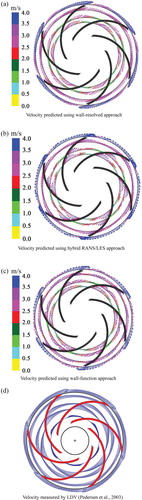
Figure 4. Velocity contours in the impeller at mid-height (z/b₂ = 0.5) from (a) the wall-resolved approach, (b) the hybrid RANS/LES approach, (c) the wall-function approach, and (d) the PIV measurements (Pedersen et al., 2003).

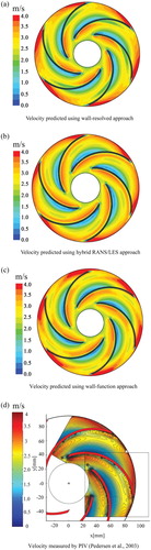
Figure 4 shows the velocity contours on the mid-height (z/b₂ = 0.5) plane of the impeller. The low-velocity zone at about 0.75R₂ near to the blade suction side is evident in the results of the wall-resolved approach, which validates the analysis above. In the results of the wall-resolved approach and the wall-function approach (see Figure 4(a) and (c), respectively), the velocities increase to the maximum value and subsequently decrease from the blade pressure side to its suction side in the middle circular direction. In the results of the hybrid RANS/LES approach (see Figure 4(b)), the maximum velocity appears close to the blade suction side. The results of the wall-resolved approach are in closer agreement with the PIV data. Different shapes of the high-velocity zone are produced by the three simulations at the outlet near to the blade pressure side. The high-velocity zones predicted by the wall-resolved approach and the hybrid RANS/LES approach are smaller than those predicted by the wall-function approach, and are closer to the PIV data.

A quantitative analysis was undertaken for the radial and tangential velocities predicted by the three approaches and the PIV measurements (Byskov, Jacobsen, & Pedersen, 2003) at the radial positions of r/R₂ = 0.5 and r/R₂ = 0.9, where the separations of the flow are obvious ( Figure 5). The horizontal coordinate is the angle of the passage. The measured averaged values are the same for each of the passages. This is the first indication that the three simulations are in good agreement with the experimental data. However, a detailed analysis reveals a slightly more accurate prediction of the flow’s behavior in a wall-resolved approach simulation. At the radial positions of r/R₂ = 0.5 (see Figure 5(a) and (b)), the radial and tangential velocities predicted by the three approaches near to the blade pressure side region are different, while they are approximately equal for the other regions. At the pressure side region, the radial and tangential velocities predicted by the wall-resolved approach are closest to the PIV data, while the result from the wall-function approach deviates greatly from the PIV data. At the radial positions of r/R₂ = 0.9 (see Figure 5(c) and (d)), good agreement of the radial and tangential velocities between the wall-resolved approach results and the experimental data is obtained, whereas a large deviation exists, especially on the blade suction side, between the wall-function approach results and the experimental data.

Figure 5. Velocities at z/b₂ = 0.5: (a) radial velocity when r/R₂ = 0.5, (b) tangential velocity when r/R₂ = 0.5, (c) radial velocity when r/R₂ = 0.9, and (d) tangential velocity when r/R₂ = 0.9.

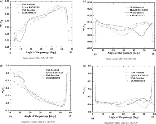
This could be interpreted as the boundary layer flow playing an important role in the whole flow in the radial positions of r/R₂ = 0.5 near to the blade pressure side and the radial positions of r/R₂ = 0.9 near to the blade suction side. To obtain the accurate flow information, the boundary layer flow must be computed. The results obtained by the wall-resolved approach and the hybrid RANS/LES approach are more significant in the separation regions, because a fine mesh is employed in the boundary layer in these two approaches. Due to the fact that the wall-function approach uses a coarse mesh in order to model the boundary layer flows by the log-law, a relatively large deviation is found in the results of the wall-function approach.

4.2. Instantaneous velocity field

In order to analyze the eddies’ generation and distribution processes, the instantaneous streamlines at the leading edge region and trailing edge region are shown in Figure 6. A separation vortex zone, caused by the fluid impinging on the blade pressure side in the blade leading edge region, is captured by each of the three approaches; however, the vortex configurations are different. Two main vortex structures distributed along the blade are captured by the wall-resolved approach on the pressure side near to the leading edge. One vortex structure is captured in the hybrid RANS/LES approach on the pressure side near to the leading edge, and it occupies a similar space to that occupied by the two vortex structures in the wall-resolved approach, but the streamlines predicted by the hybrid RANS/LES approach are smoother than those of the wall-resolved approach. In the results of the wall-function approach, no vortex structure is obviously visible and only a swinging streamline can be found. On the blade suction side at the leading edge region, only the wall-resolved approach captures some of the small vortex structures. All three approaches capture a vortex structure induced by the upstream wake on the blade pressure side in the leading edge region. The streamlines are wobbly in the results of the wall-resolved approach and wall-function approach, while the streamlines are smooth in the results of the RANS/LES approach.

Figure 6. Streamlines at the leading edge region (left) and trailing edge region (right) at Z/b₂ = 0.5 from: (a) the wall-resolved approach, (b) the hybrid RANS/LES approach, and (c) the wall-function approach.

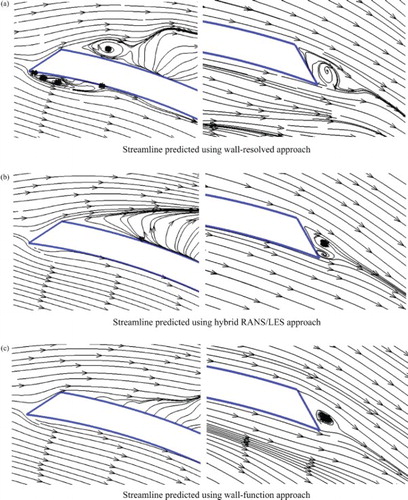
In Figure 6 the turbulent eddies are represented by the swinging streamlines. From the above analysis, it can clearly be seen that the wall-resolved approach captures the highest number of turbulent eddies, while the wall-function approach captures almost no near-wall eddies and the hybrid RANS/LES approach captures the existence of more near-wall eddies than the wall-function approach.

The fluctuated streamlines that are constituted by a fluctuated velocity are shown in the Figure 7 in order to allow analysis of the eddies’ generation and distribution processes. The fluctuated velocity is determined by subtracting the time-averaged velocity from the instantaneous velocity. The scale range of eddies from small to large, can be found in the results. The eddies’ configurations computed by the three approaches are different. Many small-sized eddies near to the blade surface are captured by the wall-resolved approach, and the small-sized eddies in the near-wall region induce more eddies in the whole impeller channel. The small-sized eddies in the near-wall region are also captured by the wall-function approach, but the eddies are fewer in number and larger than those identified by the wall-resolved approach. In the hybrid RANS/LES results there are almost no small-sized eddies near to the blade wall and the fewest eddies in the whole impeller channel are captured.

Figure 7. Fluctuated streamlines at Z/b₂ = 0.5 from (a) the wall-resolved approach, (b) the hybrid RANS/LES approach, and (c) the wall-function approach.

Since the hybrid RANS/LES approach implements the RANS method in the boundary layer, the small-sized eddies near to the blade wall cannot be captured (due to the log-law being adopted in the wall-function approach) and fewer eddies are captured by this approach. Small-sized eddies near to the blade wall in the impeller channel are captured well by the wall-resolved approach because of its accurate computation of the boundary layer.

4.3. Turbulent kinetic energy

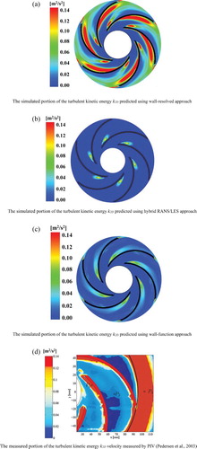
A contour plot of the portion of turbulent kinetic energy k_2D is given in Figure 8 to show the distribution of turbulent kinetic energy inside the passage. The portion of turbulent kinetic energy k_2D is defined as the time-averaged deviation of instantaneous data from the ensemble-averaged results, and it is expressed as , where and represent the RMSs of the planar velocity components. In the wall-resolved approach results, the portion of turbulent kinetic energy is generated near to the wall due to the disturbance induced by the blades. High-level turbulence areas appear downstream of the leading and trailing edges of the blade near to the suction side and downstream, and in the middle section. The distribution of the portion of turbulent kinetic energy predicted by the wall-function approach is similar to that predicted by the wall-resolved approach, but the magnitude of the portion of turbulent kinetic energy is smaller, especially on the blade suction side. In the hybrid RANS/LES approach, there is no obvious generation of turbulent kinetic energy near to the wall, except downstream of the leading edge on the blade’s pressure side. The PIV data shows that local high-level turbulence areas are confined to the near-wall areas along the blade suction side and downstream of the leading edge on the blade pressure side. By the comprehensive comparisons of the computational results with the PIV data, it can be deduced that the wall-resolved approach and wall-function approach give the best results, and that the wall-resolved approach are the most accurate of the three.

Figure 8. Portion of turbulent kinetic energy k_2D at Z/b₂ = 0.5 from (a) the wall-resolved approach, (b) the hybrid RANS/LES approach, (c) the wall-function approach, and (d) the PIV measurements (Pedersen et al., 2003).

The turbulent kinetic energy in the impeller channel includes two parts: the energy transferring from upstream and the energy generated as a result of the disturbance induced by the wall. The former is determined by the flow’s upstream characteristics and is not discussed here. The latter heavily depends on the flow in the boundary layer and is a matter of concern in this study. If turbulence characteristics such as the turbulent kinetic energy are predicted accurately then the boundary layer flow will be computed accurately. The generation and transfer values of the turbulent kinetic energy are obtained accurately, as applying the wall-resolved approach enables the detailed simulation of the boundary layer flow. The hybrid RANS/LES approach can also simulate the boundary layer flow, but the RANS – which averages the variability in the flow field – is used in the boundary layer and cannot provide enough variability fluctuation for the LES region. The log-law is adopted in order to model the boundary layer in the wall-function approach. The rough calculation of the flow in the boundary layer results in a tentative evaluation of the turbulent kinetic energy in the results of the wall-function approach. However, the results predicted by the wall-function approach are better than those of the hybrid RANS/LES approach. To obtain precise turbulent characteristics, such as the turbulent kinetic energy, the boundary layer flow must be resolved and thus the wall-resolved approach is recommended.

Future work will evaluate the near-wall solution approaches for the LES method with specific SGS models at the off-design operating conditions, wherein the rotating stall phenomena will be primarily emphasized. These predictions may also be compared with the flow field in a centrifugal pump impeller as measured by LDV and PIV (Pedersen et al., 2003).

5. Conclusions

The flow field in a centrifugal pump impeller was investigated in the near-wall region using LES methods with three approaches. For the general flow simulation such as time-averaged velocity prediction in the impeller, quantitative comparisons of the three near-wall solution approaches with PIV and LDV were performed. The wall-function approach has low resource requirements but its results are consequently of lower accuracy, and this it is not recommended for the simulation of flow with complex wall surfaces, especially flows in centrifugal impellers. The wall-resolved approach exhibits a strong performance in the computation of an impeller’s flow, although it requires a longer computation time. Using the wall-resolved approach, the stagnation and separation processes appearing on the blade suction side and downstream of the leading edge on the blade pressure side are simulated more accurately. The hybrid RANS/LES approach has a medium efficiency, with an accuracy level that falls between those of the other two approaches. The time-averaged velocity profile predicted by the hybrid RANS/LES approach is much more accurate than that of the wall-function approach.

For computing a vortex’s structure in the near-wall region of a centrifugal pump impeller, the wall-resolved approach is the best choice. If the hybrid RANS/LES method is used, some small vortex structures will not be identified, while few vortex structures can be captured in the near-wall region by the wall-function approach. The flow in the boundary layer must be resolved to determine instantaneous turbulent characteristics such as the fluctuated velocity and instantaneous turbulent kinetic energy in a centrifugal pump impeller, and this study’s findings are that in such cases only the wall-resolved approach is suitable, as the wall-function approach has been shown to not be sensitive enough, while the hybrid RANS/LES method does not give good enough results because the RANS that averages the variability in the boundary layer does not provide enough variability fluctuation for the LES region.

Disclosure statement

No potential conflict of interest was reported by the authors.

Nomenclature

	=	Resolved velocity component (m/s)
	=	Root-mean-square of the velocity fluctuations (m/s)
	=	Mean free stream velocity (m/s)
I	=	Turbulence intensity
L	=	Turbulence length scale
	=	Resolved pressure (Pa)
	=	Density (kg/m3)
	=	Kinematic viscosity (m2/s)
	=	Source terms (m/s2)
	=	SGS stress tensor (m2/s2);
	=	Resolved strain-rate tensor (1/s)
	=	SGS stress viscosity (m2/s);
	=	Magnitude of resolved strain-rate tensor (1/s);
	=	Filtered scale (m)
Cs	=	Non-dimensional model coefficient
	=	Germano identity (m2/s2);
	=	Stress on a test filter scale (m2/s2);
G	=	Production of turbulent viscosity (N/m3)
Y	=	Destruction of turbulent viscosity (N/m3)
	=	Friction velocity (m/s);
	=	Distance of this point from the wall (mm)
	=	von Kármán constant
D1	=	Inlet diameter (mm)
D2	=	Outlet diameter (mm)
b1	=	Inlet height (mm)
b2	=	Outlet height (mm)
Z	=	Number of blades
t	=	Blade thickness (mm)
	=	Inlet angle (°)
	=	Outlet angle (°)
	=	Blade curvature radius (mm)
	=	Specific speed (-)
	=	Flow rate (l/s)
H	=	Head (m)
N	=	Rotational speed (rpm)
	=	Flow rate coefficient
	=	Head coefficient
	=	Reynolds number

Additional information

Funding

This work was supported by the National Natural Science Foundation of China (grant nos. 51139007 and 51409247) and the National Science & Technology Support Project of China (grant nos. 2012BAD08B03 and 2015BAD20B01).

References

- Ansys Inc. (2009). Fluent user's guide. Retrieved from http://www.ansys.com/Products/Fluids/Ansys-Fluent
- Baggett, J. S., Jimenez, J., & Kravchenko, A. G. (1997). Resolution requirements in large-eddy simulation of shear flows. Center for Turbulence Research Stanford University, Annual Research Briefs, 51–66. doi:10.1234/12345678
- Breuer, M., Jovicic, N., & Mazaev, K. (2003). Comparison of DES, RANS and LES for the separated flow around a flat plate at high incidence. International Journal for Numerical Methods in Fluids, 41(4), 357–388. doi:10.1002/fld.445
- Byskov, R. K., Jacobsen, C. B., & Pedersen, N. (2003). Flow in a centrifugal pump impeller at design and off-design conditions—Part II: Large eddy simulations. Journal of Fluids Engineering, 125(1), 73–83. doi:10.1115/1.1524586
- Cabot, W., & Moin, P. (2000). Approximate wall boundary conditions in the large-eddy simulation of high Reynolds number flow. Flow, Turbulence and Combustion, 63(1), 269–291. doi:10.1023/A:1009958917113
- Davidson, L., & Billson, M. (2006). Hybrid LES-RANS using synthesized turbulent fluctuations for forcing in the interface region. International Journal of Heat and Fluid Flow, 27(6), 1028–1042. doi:10.1016/j.ijheatfluidflow.2006.02.025
- Davidson, L., & Dahlstrom, S. (2005). Hybrid LES–RANS: Computation of the flow around a three dimensional hill. Engineering Turbulence Modeling and Experiments, 6, 319–328. doi:10.1016/B978-008044544-1/50030-3
- Davidson, L., & Peng, S. H. (2003). Hybrid LES-RANS modelling: A one-equation SGS model combined with a k-ω model for predicting recirculating flows. International Journal for Numerical Methods in Fluids, 43(9), 1003–1018. doi:10.1002/fld.512
- Deardorff, J. W. (1970). Numerical study of three-dimensional turbulent channel flow at large Reynolds numbers. Journal of Fluid Mechanics, 41(2), 453–480. 10.1017/S0022112070000691 doi: 10.1017/S0022112070000691
- Dejoan, A., & Schiestel, R. (2001, June). Large-eddy simulation of non-equilibrium pulsed turbulent flow using transport equations subgrid scale model. Paper presented at the Second International Symposium on Turbulence and Shear Flow Phenomena, Stockholm, Sweden. Abstract retrieved from http://www.tsfp-conference.org/proceedings/2001/tsfp2-vol2-341.pdf
- Galván, S., Reggio, M., & Guibault, F. (2011). Assessment study of k-ε turbulence models and near-wall modeling for steady state swirling flow analysis in draft tube using FLUENT. Engineering Applications of Computational Fluid Mechanics, 5(4), 459–478. doi:10.1080/19942060.2011.11015386
- Germano, M., Piomelli, U., & Moin, P. (1991). A dynamic subgrid-scale eddy viscosity model. Physics of Fluids A: Fluid Dynamics, 3(7), 1760–1765. Retrieved from http://doc.sciencenet.cn/upload/file/201138125335121.pdf doi: 10.1063/1.857955
- Golshan, R., Tejada-Martínez, A. E., Juha, M., & Bazilevs, Y. (2015). Large-eddy simulation with near-wall modeling using weakly enforced no-slip boundary conditions. Computers & Fluids, 118, 172–181. 10.1016/j.compfluid.2015.06.016 doi: 10.1016/j.compfluid.2015.06.016
- Hamba, F. (2003). An approach to hybrid RANS/LES calculation of channel flow. Engineering Turbulence Modelling and Experiments, 5, 297–305. 10.1016/B978-008044114-6/50028-4
- Herbst, A. H., Schlatter, P., & Henningson, D. S. (2007). Simulations of turbulent flow in a plane asymmetric diffuser. Flow, Turbulence and Combustion, 79(3), 275–306. doi:10.1007/s10494-007-9091-5
- Jaffrezic, B., & Breuer, M. (2008). Application of an explicit algebraic Reynolds stress model within a hybrid LES-RANS method. Flow, Turbulence and Combustion, 81(3), 415–448. doi:10.1007/s10494-008-9146-2
- Jimenez, J., & Moser, R. D. (2000). LES: Where are we and what can we expect?. AIAA Journal, 38(4), 605–612. doi:10.2514/6.1998-2891
- Jones, W. P., & Wille, M. (1996). Large-eddy simulation of a plane jet in a cross-flow. International Journal of Heat and Fluid Flow, 17(3), 296–306. 10.1016/0142-727X(96)00045-8 doi: 10.1016/0142-727X(96)00045-8
- Kader, B. (1981). Temperature and concentration profiles in fully turbulent boundary layers. International Journal of Heat and Mass Transfer, 24(9), 1541–1544. 10.1016/0017-9310(81)90220-9 doi: 10.1016/0017-9310(81)90220-9
- Krajnovic, S., & Davidson, L. (2002). Large-eddy simulation of the flow around a bluff body. AIAA Journal, 40(5), 927–936. doi:10.2514/2.1729
- Lilly, D. K. (1992). A proposed modification of the Germano subgrid-scale closure method. Physics of Fluids A: Fluid Dynamics, 4(3), 633–635. doi:10.1063/1.858280
- Liu, C. H., Vafidis, C., & Whitelaw, J. H. (1994). Flow characteristics of a centrifugal pump. Journal of Fluids Engineering, 116(1), 303–309. doi:10.1115/1.2910272
- Mathey, F., Cokljat, D., Bertoglio, J. P., & Sergent, E. (2003, October). Specification of LES Inlet Boundary Condition Using Vortex Method. Paper presented at 4th International Symposium on Turbulence, Heat and Mass Transfer. Antalya, Turkey. Abstract retrieved from https://hal.archives-ouvertes.fr/hal-00274860
- Menter, F. R., Kuntz, M., & Langtry, R. (2003). Ten years of industrial experience with the SST turbulence model. Turbulence, Heat and Mass Transfer, 4, 625–632. Retrieved from http://cfd.spbstu.ru/agarbaruk/c/document_library/DLFE-6882.pdf
- Mockett, C., Fuchs, M., & Thiele, F. (2012). Progress in DES for wall-modelled LES of complex internal flows. Computers and Fluids, 65, 44–55. 10.1016/j.compfluid.2012.03.014 doi: 10.1016/j.compfluid.2012.03.014
- Nikitin, N. V., Nicoud, F., Wasistho, B., Squires, K. D., & Spalart, P. R. (2000). An approach to wall modeling in large-eddy simulations. Physics of Fluids, 12(7), 1629–1632. doi:10.1063/1.870414
- Pedersen, N., Larsen, P. S., & Jacobsen, C. B. (2003). Flow in a centrifugal pump impeller at design and off-design conditions-part I: Particle image velocimetry (PIV) and laser doppler velocimetry (LDV) measurements. Journal of Fluids Engineering, 125(1), 61–72. 10.1115/1.1524585 doi: 10.1115/1.1524585
- Piomelli, U. (2008, September). Wall-modeled large-eddy simulations: Present status and prospects. Paper presented at the 7th International ERCOFTAC Workshop on Direct and Large-Eddy Simulation, Trieste, Italy. Abstract retrieved from http://link.springer.com/chapter/10.1007/978-90-481-3652-0_1
- Piomelli, U., & Balaras, E. (2002). Wall-layer models for large-eddy simulations. Annual Review of Fluid Mechanics, 34, 349–374. doi:10.1016/j.paerosci.2008.06.001
- Piomelli, U., Balaras, E., & Pasinato, H. (2003). The inner-outer layer interface in large-eddy simulations with wall-layer models. International Journal of Heat and Fluid Flow, 24(4), 538–550. doi:10.1016/S0142-727X(03)00048-1
- Rodi, W. (1998). Large-eddy simulations of the flow past bluff bodies: State-of-the-art. JSME International Journal, Series B: Fluids and Thermal Engineering, 41(2), 361–374. doi:10.1299/jsmeb.41.361
- Schumann, U. (1975). Subgrid scale model for finite difference simulations of turbulent flows in plane channels and annuli. Journal of Computational Physics, 18(4), 376–404. doi:10.1016/0021-9991(75)90093-5
- Spalart, P. R. (2000). Strategies for turbulence modeling and simulations. International Journal of Heat and Fluid Flow, 21(3), 252–263. doi:10.1016/S0142-727X(00)00007-2
- Spalart, P. R., & Allmaras, S. R. (1992). A one-equation turbulence model for aerodynamic flows. Technical Report AIAA-92-0439, American Institute of Aeronautics and Astronautics. Retrieved from http://arc.aiaa.org/doi/abs/10.2514/6.1992-439
- Stepanoff, A. J. (1992). Centrifugal and axial flow pumps: Theory, design and application (2nd ed.). Krieger, Melbourne: John Wiley & Sons.
- Su, W. T., Li, F. C., Li, X. B., Wei, X. Z., & Zhao, Y. (2012). Assessment of LES Performance in Simulating Complex 3D Flows in Turbo-Machines. Engineering Applications of Computational Fluid Mechanics, 6(3), 356–365. doi:10.1080/19942060.2012.11015427
- Temmerman, L., Hadziabdicb, M., & Leschzinera, M. A. (2005). A hybrid two-layer URANS-LES approach for large eddy simulation at high Reynolds numbers. International Journal of Heat and Fluid Flow, 26(2), 173–190. doi:10.1016/j.ijheatfluidflow.2004.07.006
- Temmerman, L., Leschziner, M. A., & Hanjalic, K. (2002). A priori studies of near-wall RANS model within a hybrid LES/RANS scheme. Engineering Turbulence Modeling and Experiments, 5, 317–326. doi:10.1234/12345678
- Tucker, P. (2003, June). Differential equation based length scales to improve DES and RANS simulations. Paper presented at the 16th AIAA Computational Fluid Dynamics Conference, Orlando, America. doi:10.2514/6.2003-3968
- Tucker, P., & Davidson, L. (2004). Zonal k–l based large eddy simulation. Computers and Fluids, 33(2), 267–287. doi:10.1016/S0045-7930(03)00039-2
- Wang, F. J. (2004). Computational Fluid Dynamics Analysis: CFD principles & application. Beijing, China: Tsinghua University Press.
- Wang, M., & Moin, P. (2000). Computation of trailing-edge flow and noise using large-eddy simulation. AIAA Journal, 38(12), 2201–2209. doi:10.2514/2.895
- Werner, H., & Wengle, H. (1993, September). Large-eddy simulation of turbulent flow over and around a cube in a plane channel. Paper presented at the 8th International Symposium on Turbulent Shear Flows, Munich, Germany. doi:10.1007/978-3-642-77674-8_12
- Wu, X., Schluter, J., & Moin, P. (2006). Computational study on the internal layer in a diffuser. Journal of Fluid Mechanics, 550, 391–412. doi:10.1017/S0022112005008116
- Yang, Z. J., Wang, F. J., & Zhou, P. J. (2012). Evaluation of subgrid-scale models in large-eddy simulations of turbulent flow in a centrifugal pump impeller. Chinese Journal of Mechanical Engineering, 25(5), 911–918. 10.3901/CJME.2012.05.911 doi: 10.3901/CJME.2012.05.911