Hull shape optimization for autonomous underwater vehicles using CFD

ABSTRACT

Drag estimation and shape optimization of autonomous underwater vehicle (AUV) hulls are critical to energy utilization and endurance improvement. In the present work, a shape optimization platform composed of several commercial software packages is presented. Computational accuracy, efficiency and robustness were carefully considered and balanced. Comparisons between experiments and computational fluid dynamics (CFD) were conducted to prove that a two-dimensional (2D) unstructured mesh, a standard wall function and adaptive mesh refinement could greatly improve efficiency as well as guarantee accuracy. Details of the optimization platform were then introduced. A comparison of optimizers indicates that the multi-island genetic algorithm (MIGA) obtains a better hull shape than particle swarm optimization (PSO), despite being a little more time consuming. The optimized hull shape under general volume requirement could provide reference for AUV hull design. Specific requirements based on optimization testify of the platform’s robustness.

KEYWORDS:

• Computational fluid dynamics
• autonomous underwater vehicle
• shape optimization
• experiment verification

1. Introduction

Autonomous underwater vehicles (AUVs) have a broad scope in both civilian and military applications (Newman, Westwood, & Westwood, 2007; Wernli, 2000). They can integrate various sonar and sensory equipment to carry out numerous assignments such as sea bottom topography, resource prospection, searching for crashed airplanes, researching the behavior of marine wildlife and mine and submarine detection. Good endurance is essential in order to complete these missions, and many AUVs cannot reach the range or velocity desired for some purposes because of the underestimation of hull drag and/or the overestimation of propulsion. For energy utilization and endurance improvement, it is necessary to optimize AUV hulls on the basis of correct drag estimation. Streamlined hulls are adopted to make AUVs more hydrodynamically efficient, and designs focusing on body of revolution are most popular for their good performance in hull drag reduction, pressure-bearing capacity and inner space utilization. Most shape optimization work focuses on bodies of revolution.

Some prior research combining AUV drag estimation and shape optimization has been carried out. Parsons, Goodson, and Goldschmied (1974) delivered a non-gradient algorithm for body of revolution optimization in a finite constrained parameter space; however, the adopted drag estimation method was Young’s formula, which only applies to laminar flow without turbulent separation. Myring (1976) introduced a viscous–inviscid interaction method to predict body of revolution drag and analyzed drag variation as the body shape changed at the Reynolds number 10⁷. His research concluded that the body drag could not change much as the nose or tail vary from lanky to plump within a certain range, but increase dramatically once outside that range. Schweyher, Lutz, and Wagner (1996) used an evolution strategy as an optimization algorithm to get minimum-drag bodies. The flow field was modeled by a linear varying distribution of sources and sinks on the body axis. Lutz and Wagner (1998) implemented a linear stability theory to calculate the drag of axisymmetric bodies, and developed a numerical shape optimization method for minimizing the drag for a given inner space range. A semi-empirical eⁿ-method was used for transition prediction. Alvarez, Bertram, and Gualdesi (2009) implemented a first-order Rankine panel method to optimize the hull shape of an AUV operating under snorkeling conditions near a free surface.

With the development of computer technology, computational fluid dynamics (CFD) is now widely applied to analyzing AUV hydrodynamic performance. Most research is based on the Reynolds-averaged Navier–Stokes (RANS) formulation because it can treat viscous effects much better than potential flow theory and needs less computer resources than large eddy simulation (LES). Stevenson, Furlong, and Dormer (2007) compared the drag performance of seven representative revolution bodies which were all scaled to the same volume. The results suggest that a laminar flow body form could be more efficient than a torpedo form, but it was more sensitive to ancillaries and manufacturing imperfections. Sarkar, Sayer, and Fraser (1997) also made a comparison among four hull forms and found that two of the forms have superior drag performance compared to the other two. Wei, Yu, and Yang (2014) provided a detailed analysis of the drag performance of five shapes at different velocities, concluding that two are more adaptable to higher speeds and three more adaptable to lower speeds. Yamamoto (2015) and Nouri, Zeinali, and Jahangardy (2015) also carried out some related work, but their achievements are not totally applicable in other cases.

Though valuable, these various investigations have limitations with regard to engineering applications. The potential flow theory method possesses the advantage of having a high calculation speed, but it only applies to a finite constrained parameter space wherein the turbulence featu es are not obvious. Existing CFD investigations use a 3D method to obtain accurate results, but they are more time-consuming as a result. They are limited to comparisons between several standard models, which results in poor robustness. Because an AUV’s shape is inextricably bound to the mission requirements such as equipment size and maneuverability index, when scientists and engineers get the design assignment they cannot attain the ideal hull shape on account of these restrictions. This paper intends to present an improvement on this situation. Several commercial software packages have been built up into optimization platforms, with experiments being used to validate that these platforms can be employed not only for general shape analysis but also for shape optimization of specific underwater vehicles. The software packages employed in this paper are iSIGHT (Dassault Corp., 2011) Microsoft Excel, ANSYS Icem, and Fluent (ANSYS Inc., 2011a, 2011b). Several scripts and subroutines have been developed to make the optimization work automatically.

This paper is structured as follows. In section 2, the adopted 2D unstructured mesh, standard wall function and adaptive mesh strategy are introduced, along with the results of the experiments undertaken to validate that the optimization is reliable. The hull shape optimization platform is detailed in section 3, and then a few optimization results are presented in section 4 to validate the platform’s robustness.

2. Flow simulation and experimental validation

2.1. Geometrical definition

A Myring-type body was used to parameterize the AUV hull shapes. It is defined by a nose and a tail section that are connected with a middle cylindrical section. The nose is described by a modified semielliptical radius distribution as and the tail is defined by a cubic relationship as where x is the axial distance to the nose tip, a, b, and c are the lengths of the nose, middle and tail, respectively, d is the middle hull diameter, n is the index of the nose shape, and θ is the tail semi-angle. The bigger the values of n and θ, the plumper the body of revolution becomes. Figure 1 shows a schematic view of the Myring-type body. A variety of shapes can be generated by changing the six parameters a, b, c, d, n and θ.

Figure 1. Schematic view of the Myring-type body.

2.2. Numerical basis and turbulence model

The commercial software ANSYS Fluent was selected as the CFD solver. The RANS equations that solve time-average mass and moment conservation equations were used as the basis for conducting the numerical calculations. The mass continuity equation and Navier–Stokes equation are based on the assumption that incompressible fluid can be described as where x_i (i = 1, 2, 3) is the axes of the orthogonal coordinate system, is the component of the fluid velocity vector, is the water density, p is the pressure, is the viscosity stress tensor of water, and F_i is the external force along x_i. Governing equations, underlying the assumption of incompressible, isothermal and steady, were solved on the basis of finite volume method.

Figure 2. Schematic view of the Myring-type body.

A k-ω shear stress transport (k-ω SST) turbulence model was employed to make the equation set closure because this turbulence model not only provides the best prediction of vortex distribution around underwater vehicles but also strikes a good balance between computational cost and convergence stability (Dantas & Barros, 2013; de Barros & Dantas, 2012; Lloyd & Espanoles, 2002).

2.3. Mesh generation

Due to technological advancements, model tests are progressively being replaced with CFD simulation. A 3D simulation method with a structured mesh is most often employed to simulate the flow around a body of revolution. With regard to the relativity of motion, the flow past a stationary body was simulated instead of moving bodies in still water in order to enhance calculative efficiency. The outer region is a cylinder, which is concentric with the body of revolution. The cylinder length is 15 times the length of the body, and the nose is a distance of 5 times the body length from the velocity input surface and 10 times the body length from the velocity output surface. The diameter of the cylinder is about 25 times the diameter of the body (de Barros & Dantas, 2012).

Another drag calculation method is a 2D method (Zhang, Wang, & Yu, 2009), the basic principles of which are shown in Figure 2. Only a half middle section plane mesh is generated, and an axial symmetry of flow is exploited to simulate the field. The greatest advantage of this method is the high computational efficiency. If the volume grid size of a 3D model is 0.6–0.8 million cells, it would take at least 2 hours to obtain a reasonable value using a quad core CPU in parallel, whereas it only takes 5 minutes using a serial CPU when the 2D method was employed. Subsequent validation shows that the 2D method might sacrifice a little computational accuracy, with a great reduction in computational time and resources, making it a superb solution for optimization platforms.

Structured or unstructured meshes can be employed for CFD simulation. The nodes in a structured mesh are organized, and their interrelationships are clear, which provides a high level of calculation accuracy and efficiency. However, drawing a structured mesh is a waste of manpower, especially when dealing with complex geometry. By contrast, an unstructured mesh needs only a small degree of manual manipulation and can be generated in minutes. It is also adaptive to any geometry. Even though the accuracy and efficiency are not as good as with a structured mesh, this is traded off against the great saving in time and effort. Therefore, an unstructured mesh is a good choice for optimization platform construction.

The turbulence model itself is incapable of describing the flow in the near-wall region because the turbulence does not develop well. A wall function is thus employed to model the buffer sublayer in the boundary layer correctly. The height of the first layer is given by the non-dimensional wall distance y⁺, defined as where Δy is the distance between the first layer and the body surface, ρ is the water density, is the friction velocity, is the shear stress at the body surface, and and are the dynamic and kinematic viscosity coefficients, respectively. If an enhanced wall function is adopted then y⁺ should be as close to 1 as possible. If a standard wall function is adopted then a value between 30 and 60 is preferable.

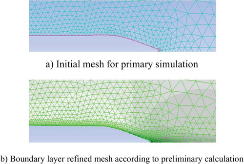
With different design programs, engineers may require different sizes and shapes of the body of revolution, and the drag needs to be minimized at cruise speed. It is also the case that a range of operational speeds could be used. This large variety of requirements would have an impact on mesh generation, affecting such parameters as the mesh size restriction and boundary layer thickness. In order to resolve this problem without manual intervention, an adaptive strategy is employed to improve the robustness of the mesh. An initial simulation is conducted, then the adaptive strategy refines or coarsens the initial mesh according to the results of the primary simulation, which in turn results in the y⁺ requirements being met. The simulation then continues using the adapted mesh. The mesh before and after adaptation is shown in Figure 3.

Figure 3. Example of mesh refinement: (a) initial mesh, and (b) refined boundary layer mesh.

2.4. Experimental validation

Captive model tests were conducted to validate the CFD simulations. The tests were carried out in the circulating water tunnel of the State Key Laboratory of Science and Technology on Autonomous Underwater Vehicles at Harbin Engineering University, China. The circulating water tunnel is 7 m in effective length, 1.5 m in depth and 1.7 m in width, with a velocity range of 0.2 m/s to 2.0 m/s. A set of models were manufactured and tested for the validation (Figure 4). They consisted of two detachable noses and tails and could all be assembled to a middle column section to form a complete body of revolution. The column diameter and length were 280 mm and 737 mm, respectively. The noses and tails were numbered from 1 to 4 with shapes based on the Myring formula (Table 1). Figure 5 exhibits the four assembled types.

Figure 4. The five sections used to create the four different test models.

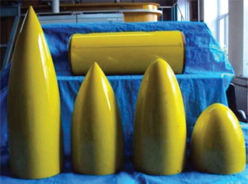
Figure 5. The four test models.

Table 1. Values for nose and tail shapes based on the Myring formula.

Nose			Tail
No.	a (mm)	n	No.	c (mm)	θ (°)
1	280	2.0	3	504	38
2	504	1.8	4	784	27

A six-component balance was fixed in the body. Two rapiers were used to connect to the balance and hold the body still while generated water flowed past it. The body was submerged in water of a depth three times the body diameter to minimize errors due to the Venturi suction force. As a further measure to minimize other effects on the drag measurements, diameter of rapiers was tapered as small as possible, 10 mm, near the body surface. Figure 6 shows the first assembly under test. The Reynolds number based on the body length ranges from 3.6 × 10⁵ to 4.2 × 10⁶, which covers the possible range of the AUV’s cruising speed. The drag variation according to the flow velocity plotted in Figure 7 indicates that the CFD result is in good agreement with the model test when the flow velocity changes from 0.3 m/s to 1.5 m/s. The measured value is significantly greater than the CFD result when the velocity is higher than 1.5 m/s, as the flow generated by the circulating water tunnel is more turbulent than the flow in the CFD code.

Figure 6. The first model under test conditions.

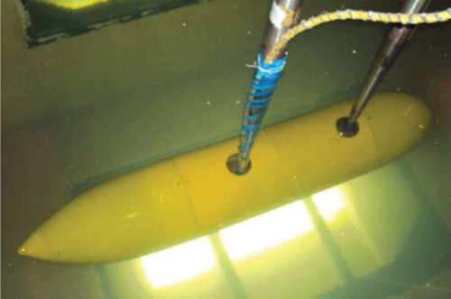
Figure 7. Comparison of drag versus flow velocity for CFD simulation and experimental results.

The experiments conducted using the other three models revealed the same trend. This validation work demonstrates that the numerical simulation procedure can model experiments with an acceptable level of accuracy, and that an optimization platform based on this procedure will be reliable.

3. Hull shape optimization methodology

The hull shape optimization methodology has special requirements for both the mesh generation and the solver strategy, which should adapt to geometry change and velocity variation. The solver should also obtain accurate results with high performance in order to make the platform efficient. According to previous experiments and validation, a 2D triangle mesh and related solver, a k-ω SST turbulence model, a standard wall function and an adaptive strategy were employed. While this configuration does sacrifice a little accuracy, the calculation speed is greatly improved.

3.1. Optimization method and procedure

The definition of the complete optimization procedure is shown in Figure 8. The optimization platform is structured in only one tier: hydrodynamic drag. The iSIGHT program is responsible for controlling the process and assigning the values of the parameters. The calculation and setting of the parameters in this step ensures that the specific size requirements are fulfilled. Microsoft Excel with embedded Visual Basic for Applications (VBA) code receives the parameters and generates the volume and coordinates for the curves of the body of revolution. If the volume value comes within the predefined range then a corresponding shape file is exported. ANSYS Icem then reads the file and generates the initial 2D mesh in Fluent in order to carry out a primary simulation. According to the primary result, the mesh refinement is increased or decreased and a subsequent iteration is conducted. This is beneficial for getting an authentic drag value, which has strong implications on optimization reliability.

Figure 8. Flow chart of the optimization procedure.

3.2. Optimizer comparison and selection

As a central section of the platform, the optimization algorithm is critical to efficiency and precision. Some algorithms may run less iterations but obtain an unfavorable outcome, while others can produce a good final result but take weeks to finish executing. In this study, particle swarm optimization (PSO; Kennedy, 2010) and a multi-island genetic algorithm (MIGA; Holland, 1975) were applied separately to the optimizer in order to understand their advantages and disadvantages. To make the optimization algorithms comparable, identical geometric restrictions on the basis of above-mentioned experiment and general AUV design requirements were used (Table 2).

Table 2. Range of design parameters for shape optimization.

Parameter		Minimum	Maximum
Diameter of middle section	d	100 mm	500 mm
Length of nose section	a	0.5d	1600 mm
Length of middle section	b	50 mm	1400 mm
Length of tail section	c	d	1500 mm
Index of nose shape	n	0.6	3.0
Tail semi-angle	θ	5°	40°
Displacement volume	vol	0.09 m^3	0.15 m^3
Total length	l = a + b + c	–	10d

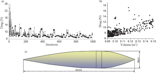
As well as the consistent geometry, the same inlet velocity and water properties were defined. Convergent process comparisons and data point distributions are shown in Figures 9 and 10. The PSO algorithm converged within only a few iterations and then the drag values kept oscillating in a wide range during the subsequent iterations and converged no further. The MIGA optimization changed periodically because genetic variation was implanted. The drag values converged during each period. The PSO algorithm calculated a limited number of times, resulting in a uniform distribution of the data points in the computing space. The optimization procedure showed no obvious tropism. The MIGA took longer but it was a consistently perfect process; the optimization distinctly approaches the ideal outcome. Comparing the optimization results, the minimum drag shape obtained using the MIGA is 3.4% less than the shape obtained using the PSO algorithm.

Figure 9. Convergence results of PSO optimization: (a) iterative procedure, (b) data point distribution, and (c) minimum drag shape.

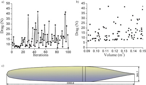
Figure 10. Convergence results of MIGA optimization: (a) iterative procedure, (b) data point distribution, and (c) minimum drag shape.

4. Optimization results

4.1. Optimization based on general volume requirements

According to the calculation results from Figure 10(b), each revolution body volume corresponds to a minimum drag, and this drag value increases with the volume in an approximately linear fashion. More calculations were conducted to figure out the minimum drag change rule with volume variation at different cruising speeds. Figure 11 shows the minimal drag variation along the body volume and the basic form of the minimum drag body. The optimization result indicates that as long as the displacement volume increases, the body drag becomes higher. This trend is more palpable at higher speeds; thus, the volume of the body of revolution should be as small as possible, especially when it is designed to cruise at higher speeds.

Figure 11. Optimization results: (a) minimal drag curves at different speeds and (b) best body of revolution shape for standard requirements.

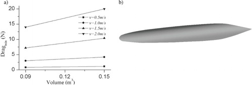
The drag which the body of revolution suffered in fluid can be divided into friction drag and viscosity drag. Friction drag varies with body speed and wetted surface area, and viscosity drag is strongly dependent on the pressure gradient. The optimization result illustrates that drag reduction is all about reducing the surface area and minimizing flow separation. For a preferable low drag body of revolution, the inner space of the AUV should be minimized; there should be a longer nose section, and a tail section of reasonable size, with the middle section as small as possible. Such a hull form can promote laminar flow around the body boundary layer and decrease energy diffusion.

4.2. Optimization based on specific requirements

Many factors should be considered when defining the parameters for the body of revolution for particular AUVs, e.g., the minimum body diameter is limited by size of the largest pieces of equipment, the total weight of the equipment and the buoyancy of the materials used, which determines the volume of inner space required, while the general arrangement of the equipment affects the length range of the nose, middle and tail sections. The requirements of metacentric height, maneuverability and seakeeping performance when working near a free surface should also be taken into consideration. A good optimization platform should be capable of generating a body of revolution whose drag is minimal under different sets of requirements.

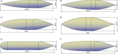
To validate the platform robustness, several sets of requirements were imported into the optimization platform separately. Figure 12 shows the best body of revolution shape under different sets of requirements; the middle section is extremely small, so the body basically consists of a longer nose and an appropriate tail. This body shape results in a gradual increase in diameter, creating a desirable pressure gradient over the nose part that promotes laminar flow within its boundary layer, which makes the skin friction drag much lower than a turbulent boundary layer. The optimization platform is implemented on an Intel Core CPU i5-4590 @3.3 GHz. Approximately 1000 iteration steps are carried out, requiring a computational time of about 5 days. In comparison, a conventional 3D method would take over 2 months, which is obviously much too long a time.

Figure 12. Best body of revolution shape under different sets of requirements (after part (a), only the values which differ from those of part (a) are stated): (a) u = 1.0 m/s, 200 mm < a < 1600 mm, 50 mm < b < 1400 mm, 100 mm < c < 1500 mm, 100 mm < d < 500 mm, 0.6 < n < 3, 5° < θ < 40°, l < 7d, 0.09 m³ < Vol < 0.15 m³, (b) l < 6d, (c) l < 5d, (d) l < 4d, (e) u = 2.0 m/s, 200 mm < a < 300 mm, 400 mm < b < 1400 mm, 300 mm < c < 1500 mm, 200 mm < d < 400 mm, l < 8d, (f) u=2.0 m/s, a<3d, c<3d.

Note: For all six examples, 0.6 < n < 3, 5° < θ < 40°, 0.09 m³ < vol < 0.15 m³.

5. Conclusion

This paper presents an optimization platform for AUV hull shapes, in which an unstructured 2D mesh, standard wall function and adaptive mesh strategy are applied to calculate the direct route drag of bodies of revolution. Its use can greatly improve computational efficiency. The accuracy of the optimization platform is proved by experimental validation to be robust and effective. According to the optimization results, the traditional AUV hull shape with a long cylinder as the middle part is not a good option for drag reduction. The optimal choice, in the simulated velocity range, is basically a body of revolution with a long nose, a minimal middle section, and an appropriate tail. When the best options cannot be chosen due to a particular restriction, optimization still be carried out to improve AUV hydrodynamic performance within the limitations.

Compared to the recently published research by Vasudev, Sharma, and Bhattacharyya (2014, 2015), the work in this paper has definite advantages in engineering application because of its efficiency and robustness. This paper aimed to construct a platform for AUV hull shape optimization, but only primitive PSO and MIGA methods were adopted and compared. Future work can focus on improving efficiency in two stages: 1) implement parallel computation to allow the computer to work at full capacity, and 2) identify more suitable optimization algorithms such as those used in Taormina and Chau (2015) and Zhang and Chau (2009).

Acknowledgements

The efforts of members of the Science and Technology Laboratory on Autonomous Underwater Vehicles are gratefully acknowledged.

Disclosure statement

No potential conflict of interest was reported by the authors.

Additional information

Funding

This work is supported by the Postdoctoral Science Foundation of China [grant no. 2014M561333] and the National Nature Science Foundation of China [grant no. 51579022].

References

- Alvarez, A., Bertram, V., & Gualdesi, L. (2009). Hull hydrodynamic optimization of autonomous underwater vehicles operating at snorkeling depth. Ocean Engineering, 36(1), 105–112. doi: 10.1016/j.oceaneng.2008.08.006
- ANSYS Inc. (2011a). ANSYS Fluent 13.0 user's guide. Canonsburg, PA: ANSYS Inc.
- ANSYS Inc. (2011b). ANSYS Icem 13.0 user's guide. Canonsburg, PA: ANSYS Inc.
- Dantas, J. L. D., & Barros, E. A. d. (2013). Numerical analysis of control surface effects on AUV manoeuvrability. Applied Ocean Research, 42, 168–181. doi:doi: 10.1016/j.apor.2013.06.002
- de Barros, E., & Dantas, J. L. D. (2012). Effect of a propeller duct on AUV maneuverability. Ocean Engineering, 42, 61–70. doi: 10.1016/j.oceaneng.2012.01.014
- Dassault Corp. (2011). iSIGHT 5.6 design gateway and runtime gateway help. Cary, NC: Dassault Systémes Simulia Corp.
- Holland, J. H. (1975). Adaptation in natural and artificial systems. Ann Arbor, Michigan: University of Michigan Press.
- Kennedy, J. (2010). Particle swarm optimization. In Encyclopedia of machine learning (pp. 760–766). New York, NY: Springer.
- Lloyd, G., & Espanoles, A. (2002). Best practice guidelines for marine applications of computational fluid dynamics. WS Atkins Consultants and Members of the NSC, MARNET-CFD Thernatic Network.
- Lutz, T., & Wagner, S. (1998). Drag reduction and shape optimization of airship bodies. Journal of Aircraft, 35(3), 345–351. doi: 10.2514/2.2313
- Myring, D. F. (1976). A theoretical study of body drag in subcritical axisymmetric flow. Aeronautical Quarterly, 27(3), 186–194. doi: 10.1017/S000192590000768X
- Newman, P., Westwood, R., & Westwood, J. (2007). Market prospects for AUVs. Marine Technology Reporter, 50(8), 22–24.
- Nouri, N. M., Zeinali, M., & Jahangardy, Y. (2015). AUV hull shape design based on desired pressure distribution. Journal of Marine Science & Technology, 1–13. 10.1007/s00773-015-0343-0
- Parsons, J. S., Goodson, R. E., & Goldschmied, F. R. (1974). Shaping of axisymmetric bodies for minimum drag in incompressible flow. Journal of Hydronautics, 8(3), 100–107. doi: 10.2514/3.48131
- Sarkar, T., Sayer, P. G., & Fraser, S. M. (1997). A study of autonomous underwater vehicle hull forms using computational fluid dynamics. International Journal for Numerical Methods in Fluids, 25(11), 1301–1313. 10.1002/(SICI)1097-0363(19971215)25:11 doi: 10.1002/(SICI)1097-0363(19971215)25:11<1301::AID-FLD612>3.0.CO;2-G
- Schweyher, H., Lutz, T., & Wagner, S. (1996). An optimization tool for axisymmetric bodies of minimum drag. Paper presented at the 2nd International Airship Conference, Stuttgart/Friedrichshafen.
- Stevenson, P., Furlong, M., & Dormer, D. (2007). AUV shapes-combining the practical and hydrodynamic considerations. Paper presented at the OCEANS 2007-Europe.
- Taormina, R., & Chau, K.-W. (2015). Neural network river forecasting with multi-objective fully informed particle swarm optimization. Journal of Hydroinformatics, 17(1), 99–113. doi: 10.2166/hydro.2014.116
- Vasudev, K. L., Sharma, R., & Bhattacharyya, S. (2014). A CAGD+CFD integrated optimization model for design of AUVs. Paper presented at the OCEANS 2014-TAIPEI.
- Vasudev, K. L., Sharma, R., & Bhattacharyya, S. K. (2015). An optimization model incorporating clash free mechanism for design of AUVs. Paper presented at the Underwater Technology (UT), 2015 IEEE.
- Wei, Z., Yu, Q., & Yang, S. (2014). Analysis of the resistance performance for different types of AUVs based on CFD. Chinese Journal of Ship Research, 9(3), 28–37. doi: 10.3969/j.issn.1673-3185.2014.03.004
- Wernli, R. L. (2000). AUVs – the maturity of the technology.
- Yamamoto, I. (2015). Research on next autonomous underwater vehicle for longer distance cruising. IFAC-PapersOnLine, 48(2), 173–176. doi: 10.1016/j.ifacol.2015.06.028
- Zhang, J., & Chau, K. W. (2009). Multilayer ensemble pruning via novel multi-sub-swarm particle swarm optimization. Journal of Universal Computer Science, 15(4), 840–858. doi: 10.3217/jucs-015-04-0840
- Zhang, X., Wang, S., & Yu, D. (2009). 2D axisymmetric CFD simulation of underwater torpedo launch tube flow. Paper presented at the 2009 International Conference on Information Engineering and Computer Science.