Numerical modeling of oscillating Taylor bubbles

ABSTRACT

In this study, computational fluid dynamics (CFD) modeling is used to simulate Taylor bubbles rising in vertical pipes. Experiments indicate that in large diameter (0.29 m) pipes for an air–water system, the bubbles can rise in a oscillatory manner, depending on the method of air injection. The CFD models are able to capture this oscillatory behavior because the air phase is modeled as a compressible ideal gas. Insights into the flow field ahead and behind the bubble during contraction and expansion are shown. For a bubble with an initial pressure equal to the hydrostatic pressure at its nose, no oscillations are seen in the bubble as it rises. If the initial pressure in the bubble is set less than or greater than the hydrostatic pressure then the length of the bubble oscillates with an amplitude that depends on the magnitude of the initial bubble pressure relative to the hydrostatic pressure. The frequency of the oscillations is inversely proportional to the square root of the head of water above the bubble and so the frequency increases as the bubble approaches the water surface. The predicted frequency also depends inversely on the square root of the average bubble length, in agreement with experimental observations and an analytical model that is also presented. In this model, a viscous damping term due to the presence of a Stokes boundary layer for the oscillating cases is introduced for the first time and used to assess the effect on the oscillations of increasing the liquid viscosity by several orders of magnitude.

KEYWORDS:

• Numerical simulation
• Taylor bubble
• bubble rise
• oscillations
• stokes boundary layer

1. Introduction

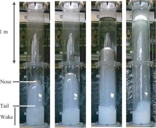
Numerous experimental studies have investigated the rise of elongated, bullet-shaped gas bubbles in pipes charged with either stagnant fluids (e.g., Figure 1) or cocurrent flows. These bubbles, called Taylor bubbles, are a key feature of the slug flow regime commonly seen in multiphase flows in the industrial context. They also occur in nature; for example, Parfitt (2004) states that Strombolian-type volcanic eruptions are widely accepted to be driven by the rise and burst of large Taylor bubbles. Taylor bubbles have attracted a great deal of interest, including the characterization of the rise rate of the bubbles (Davies and Taylor, 1950; Dumitrescu, 1943) and the determination of the flow fields ahead of (Nogueira, Riethmuler, Campos, and Pinto, 2006a), in the liquid film around (Brown, 1965) and in the wake region behind (Nogueira, Riethmuller, Campos, and Pinto, 2006b) the bubbles. Others have investigated the change of bubble shape within liquids of different transport properties (e.g., Kang, Quan, and Lou, 2010).

Figure 1. A variety of experimentally-produced Taylor bubbles ranging in length from 0.3 m to over 1 m. For the shortest bubble, the approximate positions of the nose, tail and wake regions are indicated.

In this paper, commercial computational fluid dynamics (CFD) software is used to simulate the flow observed in the experiments detailed in Pringle, Ambrose, Azzopardi, and Rust (2015), with the ultimate goal of producing a validated model suitable for running simulations under conditions that are difficult to create in a laboratory (e.g., larger-scale, higher-dynamic viscosity).

The experiments of Pringle et al. (2015) were conducted in a vertical Perspex pipe 10 m in length and with an internal diameter of 0.29 m. The pipe was partially filled with water and open to the atmosphere at the top. Compressed air was injected into the base of the pipe via a system of nozzles, with the ensuing small bubbles coalescing into a Taylor bubble. Examples of the range of bubble lengths that were produced are shown in Figure 1.

These air–water Taylor bubbles theoretically have a Froude number, Fr, of 0.351, an Eötvös number, Eo, of and a Morton number, M, of . These dimensionless numbers are, for completeness, (1) (2) (3)

where w is the vertical component of the rise velocity, g is the acceleration due to gravity, D is the diameter of the pipe, ρ is the density of the liquid, μ is the dynamic viscosity of the liquid and σ is the surface tension. The rise velocity of the bubble is assumed to be in the ‘Independent of viscosity and surface tension’ regime proposed by White and Beardmore (1962, Figure 6, p. 357) and the bubble rise rates observed by Pringle et al. (2015) are consistent with theoretical predictions and empirical models for this regime (Dumitrescu, 1943; Viana, Pardo, Yanez, Trallero, and Joseph, 2003).

Pringle et al. (2015) demonstrated that if air is injected into quiescent water then Taylor bubbles can exist in pipes that are 0.29 m in diameter, which is significantly larger than previously suggested for the air–water system. They further went on to show that if the gas injection ends abruptly then the bubble length and apparent rise rate oscillate. The oscillation frequency is lower for longer bubbles and as the bubble rises through the fluid, the frequency of the oscillations increases and the amplitude decreases. This is because as the head of the water above the rising bubble decreases, so does the force required to displace it.

This oscillatory behavior, similar to that observed in the experiments reported by Pringle et al. (2015), has been inferred to occur within volcanoes during Strombolian-type eruptions. Vergniolle, Brandeis, and Mareschal (1996) recorded acoustic pressure in the air during a period of explosive activity at the Stromboli volcano and observed oscillations in these readings during the rise of the bubble before eruption. They present a theoretical model for these oscillations, which is derived from the assumption that the bubble behaves as a simple harmonic oscillator. A similar derivation is presented in Pringle et al. (2015) and an alternative derivation is presented in section 2 of this paper.

The only other experimental study to report oscillations as a Taylor bubble rises through liquid in a tube is James, Lane, Chouet, and Gilbert (2004), who recorded these oscillations with pressure measurements at the interior wall of the tube. Their interpretations of these data are qualitative but are consistent with the model solutions of Pringle et al. (2015) and Vergniolle et al. (1996). Such oscillations have generally not been observed in previous CFD studies of Taylor bubbles because the air is modeled as incompressible. The work is continued in James, Lane, and Corder (2008), who present solutions validated by experimental data, which show that the liquid surface rises due to bubble expansion as the bubble moves into regions of lower hydrostatic pressure. They confirm that slug oscillations occur when an initial gas overpressure is used; however, no detail is provided. In this paper, CFD software is used to model and gain a better understanding of this oscillatory behavior.

It should be noted that the oscillations seen in these bubbles that result in the displacement of the column of water ahead of the Taylor bubbles should not be confused with any oscillations seen at the rear of the bubble. Numerous studies, notably Polonsky, Barnea, and Shemer (1999) and Hayashi, Hosoda, Tryggvason, and Tomiyama (2014), have focused on the changing shape of the rear of the bubble. This effect is due to the relatively high-speed falling wall film around the bubble emerging as an annular jet into the fluid behind the bubble. The oscillations that are discussed in the present work result from an initial imbalance between the internal pressure in the bubble and the local hydrostatic pressure. The bubble expands and contracts depending on the sense of this imbalance and since the water below the bubble cannot be moved, the water above the bubble is moved bodily upwards. This is confirmed by the observation that the free surface above the bubble moves in phase with the motion of the nose of the bubble (Pringle et al., 2015). Further, it has been known since Dumitrescu (1943) that the rate of rise of a Taylor bubble is determined by the hydrodynamics of the liquid above it. And, since the liquid film around the bubble cannot transport appreciably more fluid during the expansion/contraction of the bubble, the liquid must be pushed ahead of the bubble, ostensibly as a plug flow.

In recent years, CFD studies using the volume of fluid (VOF) multiphase model have replicated observations from experimental studies such as bubble rise rate and wake behavior (Araujo, Miranda, Pinto, and Campos, 2012; James et al., 2008; Ndinisa, Wiley, and Fletcher, 2005; Taha and Cui, 2004). Other interface reconstruction schemes have been used to model the gas–liquid interface. For example, Suckale, Nave, and Hager (2010) developed a numerical model using a level-set method and an analysis of these results suggest that a stable bubble cannot be sustained above a Reynolds number of 100. This corresponds to a maximum pipe diameter of less than 0.01 m for a water–air system, which is contrary to the findings of many experimental studies. James, Llewellin, and Lane (2011) questioned whether this discrepancy is the result of a physical instability or a numerical instability, and pointed out that the simulations were terminated by numerical divergence and not by a physical mechanism. Kang et al. (2010) used a front-tracking method to successfully simulate the rise of Taylor bubbles in 2D axisymmetrical pipes, but no studies have used this method to model 3D Taylor bubbles. Lu and Prosperetti (2009) also simulated axisymmetric Taylor bubbles rising through liquids in a vertical tube, but their model neglected the flow in the gas and tracked the interface using a set of marker points linked by cubic splines.

Recently, Yan, Zhang, and Che (2012) addressed the problem of small dispersed bubbles in slug flow by applying a coupled system of equations that allows different length-scales to be resolved for the different regimes – one length-scale for the Taylor bubble, modeled using a VOF model, and a different length-scale for the much smaller, dispersed bubbles in the wake. They model these small bubbles using a mixture model, which is commonly used to model the bubbly flow regime. Other similar models have been developed, such as the Hybrid Interface RESolving-Two Fluid Model of Marschall, Hinrichsen, and Polifke (2008). Neither of these approaches are pursued in the present work due to the encouraging results seen with the approach used.

CFD studies such as Taha and Cui (2004) and Araujo et al. (2012) have produced Taylor bubbles with the rise velocity agreeing with that predicted by Dumitrescu (1943). These studies use an approach in which the Taylor bubble is held at a constant position by having walls move vertically downwards around it. This approach does not take into consideration the hydrostatic pressure experienced by the bubble, nor does it include the free surface at the top of the liquid column, so it cannot be used to model the expansion and oscillatory behavior reported in the experiments of Pringle et al. (2015). Instead, the entire flow domain must be modeled, a method previously used by James et al. (2008). It is noted that the bubble rise rate simulated in that study was 15 to 20% slower than the experimental rise velocity.

It should be mentioned that other numerical approaches such as Lattice Boltzmann techniques have been applied to the modeling of Taylor bubbles (Ghosh, Patil, Mishra, Das, and Das, 2012; Yang, Palm, and Sehgal, 2002), although these are often at much smaller scales than the bubbles discussed in this paper.

The paper now continues by describing an analytical model for bubble rise and oscillation and presents an analysis and discussion of the model's predictions in section 2. This is followed in section 3 by a review of the CFD methods used, particularly the VOF model. Using this approach, an investigation is presented that compares the rise rate of non-oscillatory bubbles with existing correlations, the analytical model and the experimental work of Pringle et al. (2015). Additionally, Appendix 1 describes a validation of the CFD modeling techniques in relation to the experimental results of van Hout, Gulitski, Barnea, and Shemer (2002). In section 4, all aspects of the numerical simulations are examined, including the sensitivity of the oscillation frequency to the bubble length and initial pressure. The way in which oscillations are damped by means of an increase in the dynamic viscosity of the liquid when the Morton number approaches those seen in volcanic conduits is shown. Finally, section 5 presents the conclusions drawn from the work.

2. The bubble rise and oscillation model

Consider the situation presented in Figure 2(a). A vertical tube of diameter D contains a cylindrical bubble of length L, the top of whose nose is positioned at a distance H below the surface of the water. The bubble is rising at a given velocity, , but may be considered to be stationary in the first part of the following argument. The pressure, , in the bubble is assumed to be given by the ideal gas law (4) where n is the number of moles of the constituent gases (considered fixed), is the universal gas constant, T is the temperature (considered fixed), and V is the volume of the bubble. If the pressure in the bubble is equal to the hydrostatic pressure at its top (or nose) then the bubble will not oscillate. Note that L is the equilibrium length of the bubble, defined as being the unperturbed length of the bubble, this length being defined by the hydrostatic pressure at the nose of the bubble.

Figure 2. Schematic of the idealized Taylor Bubble in (a) its equilibrium state and (b) with the bubble length perturbed by the small amount h.

When the pressure in the bubble is perturbed by a small (say, positive) amount above the hydrostatic pressure, this results in an increase in the bubble length of h, with , as shown (in an exaggerated form) in Figure 2(b). Any elongation takes place at the nose of the bubble because any bubble expansion is precluded at the tail due to the presence of the lower wall of the tube. The plug of liquid above the bubble is therefore moved upwards at the velocity . It is assumed that there is no flow of liquid in the film that, in reality, exists around the bubble.

Since the bubble expands according to Equation (4(4) ), for a small change in length, h, (5)

Womersley (1955), in his seminal work on the pulsatile flow in arteries, proposed the dimensionless number (6) where α is now known as the Womersley number in his honor, R is the radius of the pipe, Ω is the angular frequency of the pulsing flow and ν is the kinematic viscosity. The Womersley number is the ratio of the transient inertial force to the viscous force. When , with inertial effects dominating, the ‘flow is essentially one of piston-like motion with a flat velocity profile’ (Ku, 1997, p. 402). For the water flow considered in the present work, the motion is clearly in the piston-like or plug flow regime.

There are viscous forces acting on the plug of water above the bubble as it moves up and down inside the tube. The plug of liquid which oscillates above the bubble is analogous to the situation in which a Stokes boundary layer is found – with an oscillatory flow next to a solid wall. So, if the plug of water is moving bodily as (7) where is the amplitude of the velocity variation in the oscillatory flow, the velocity component tangential to the wal, at a given point near the wall of the tube varies as (8) where y is the wall-normal coordinate and κ is a wavenumber (9) The wall shear stress is given by (10) The derivative is evaluated as (11) where it is seen that is a phase-shifted version of the velocity of the forcing oscillation (or plug rise and fall in this application, Equation (7(7) )). While, at present, it is assumed that the bubble is stationary, it should be noted that it is also assumed that this oscillatory boundary layer is formed even when the height of the plug of liquid decreases as the bubble rises. In this case, the assumption is made that even as the frequency of oscillation changes, the timescales for the boundary layer to develop are shorter.

A simple application of Newton's Second Law to the perturbed, upper plug of water reveals (12) where the terms on the right-hand side are the forces due to the pressure acting on the lower and upper surfaces of the plug, the wall shear stress and gravity, respectively. Rearranging Equation (12(11) ) gives (13) with a natural frequency (14) and a critical damping coefficient (15) The critical damping coefficient arises from the substitution of Equation (11(10) ) into Equation (10(9) ) and thence substituting for in Equation (12(11) ). Ignoring the phase shift in Equation (11(10) ) it can be seen that .

These results are equivalent to those found using similar methods by Pringle et al. (2015), Oguz and Prosperetti (1998) and Vergniolle et al. (1996), although damping was only considered by Oguz and Prosperetti. In addition, Oguz and Prosperetti found on analysis that the viscous damping is insignificant, although their bubbles are several orders of magnitude smaller than the ones being considered here. They also demonstrate that, in the limit , the critical damping coefficient ζ becomes (16) which is derived via the wall shear stress for Poiseuille flow. This has consequences when the Morton number is increased as the dynamic viscosity increases dramatically, as is observed in volcanic conduits.

To this point, the bubble has been assumed to be stationary. Clearly however the bubble is rising, so if a constant rise velocity is now assumed it can be calculated in this particular regime from (17)

which in this case gives a rise velocity of 0.59 ms⁻¹. So, H and L in Equation (14(13) ) are now functions of time, with , trivially. Again assuming the ideal gas law for the bubble and an initial length it can be shown that the equilibrium length varies as (18) where is the initial height of the water plug. As closed analytical solutions of Equation (13(12) ) are difficult since the coefficients are now both functions of time, a numerical solution is required. The ode45 ordinary differential equation solver in MATLAB (2012) was used to solve this equation. Figure 3 shows various outputs from the model using a parameter set based on the experimental work of Pringle et al. (2015) (see Table 1). In Figure 3 it can be seen that the length is normalized by the tube diameter D, the velocity is normalized by the initial velocity , and the time is normalized by the ratio .

Figure 3. Variation for the analytical oscillating bubble model of non-dimensionalized time against non-dimensionalized (a) bubble length and liquid column height, (b) angular frequency and critical damping coefficient, (c) surface velocity, and (d) surface displacement.

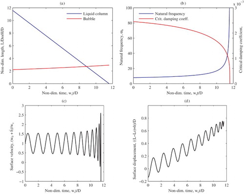
Table 1. Parameter set used for model testing from Pringle et al. (2015).

Initial height of water plug,	3.36	m
Initial equilibrium length of bubble,	0.64	m
Initial length decrease below equilibrium	0.04	m
Radius of pipe	0.145	m
Atmospheric pressure	101325	Pa
Density of water	1000	kgm^−3
Dynamic viscosity of water	0.001	kgm^−1 s^−1
Bubble rise velocity,	0.591	ms^−1

In Figure 3(a), the liquid column length decreases linearly during the bubble rise to zero as the bubble breaks the surface. As the bubble rises, the equilibrium bubble length increases according to Equation (18(17) ). The bubble, in this example, is initially under-pressured (below the hydrostatic pressure) and so the initial surface displacement h is less than zero; Figure 3(d) shows the oscillation superimposed on the increase in the equilibrium length of the bubble as it rises – without oscillation, the surface would rise due to the decompression of the rising bubble. As the bubble approaches the surface, the amplitude of the oscillation decreases, while the frequency increases (Figure 3(b)). Both predictions are consistent with the assumptions made in the derivation of the analytical model. Near to the surface the model predicts ever-increasing frequencies, but in reality the breaking process prevents the bubble reaching this point with an identifiable plug of liquid above it.

Figure 3(c) shows the normalized surface velocity, which is a superposition of bubble rise velocity, and . This confirms the experimental observation that the bubble appears to rise in a uneven manner, accelerating and decelerating as it goes. In fact, this is seen at the nose of the bubble – the tail of the bubble continues to rise at the velocity . The critical damping coefficient in this case is throughout most of the rise and therefore the damping is negligible. The critical damping coefficient quickly tends to zero as the height of the liquid plug tends to zero (Figure 3(b) and Equations (15(14) ) and (14(13) )). Any reduction in the amplitude of the oscillations is entirely due to the decrease in and not the damping, at least in this case.

3. Numerical model

In this study, the commercial CFD solver ANSYS (n.d.) FLUENT v12.1 is used.

3.1. Governing equations

The solver uses a finite-volume method to solve the momentum and continuity equations. The continuity equation is derived by applying conservation of mass to a finite volume. The momentum equations (Navier–Stokes equations) are derived from an application of Newton's Second Law. This constraint requires that the rate of change of momentum acting on the particle be equal to the sum of the forces acting upon it. Due to the turbulent nature of the flow in the wake region behind the Taylor bubble, the unsteady Reynolds-averaged Navier–Stokes (URANS) equations are used: (19) (20) where is the velocity, p is the pressure, ρ is the density, is the surface tension force, and μ and are the dynamic and turbulent eddy viscosities, respectively. Here, , p and ρ represent time-averaged quantities.

In the RANS approach, the flow variables, such as pressure, velocity and density, are split into mean and fluctuating components, which are then ensemble-averaged. The result of this is an additional term to represent the effects of turbulence in the flow, hence a model is needed to close the equations. Preliminary studies on the air–water system studied here show that the realizable (RKE) model (Shih, Liou, Shabbir, Yang, and Zhu, 1995) is the most suitable turbulence model to use for this application, given the constraints of the available computational power.

The rationale for using URANS – an approach that is often criticized by practitioners who use, for example, large eddy simulation (LES) methods – is as follows. First, the computational resources were not available to perform an acceptable LES, and second, this study is largely concerned with accurately capturing the oscillations of the bubbles and not, in particular, the wake behind the bubble. While it is clear from the results that the progression will be to show that the breakup at the tail of the bubble is not resolved as accurately as it might be using an LES and a finer grid, the flow at the nose of the bubble and in the Stokes boundary layer is accurately modeled using the chosen URANS model. Indeed, around the rising Taylor bubble, thin shear layers of liquid are seen, which then form jets behind the bubble. Further evidence to support the application of this model is presented in section 3.2.

However, inaccuracies in the modeling of the wake may result in an error in the calculated rate at which volume is lost from the bubble, which will result in a reduction in its length. Nevertheless, it has been shown that the length of the bubble does not materially affect its rise rate. What would be affected is the frequency of oscillation because this does depend on the length of the bubble and is something that will be discussed later in the paper.

The RKE model has two transport equations – one for the turbulent kinetic energy, k, and one for the dissipation rate, : (21) (22) where S is the modulus of the mean rate of strain tensor, ν is the kinematic viscosity and and are the turbulent Schmidt numbers. In this model, is given by (23) where . The remaining model constants, , and have been determined empirically and have values of 1.9, 1.0 and 1.2, respectively. The turbulent eddy viscosity is (24) as in the standard model. In the realizable model, is not a constant but is calculated using the mean strain rate and the rates of rotation (Shih et al., 1995).

A multiphase model, capable of producing a distinct interface between the gas and liquid phases, is also required. The VOF method is one of the most common methods for representing the slug flow regime using CFD. It models the interface by solving a continuity equation for the gas volume fraction in each cell: (25) where is the volume fraction of gas (Hirt and Nichols, 1981). Here it is assumed that there is no mass transfer between the phases. The liquid volume fraction is then calculated by observing the constraint (26) where is the volume fraction of liquid, which must be satisfied to conserve mass. An explicit formulation of the VOF allows the use of a ‘geometric reconstruction’ scheme to reconstruct the interface, based on the ‘piecewise linear interface calculation’ (PLIC) method (Youngs, 1982). This approach does not produce the smearing at the interface seen in other, implicit methods – it does, however, mean that an upper bound is placed on the size of the time step that can be used.

Although RANS turbulence models were principally developed to study single-phase flows, it is suggested that their application to modeling multiphase flows should be considered. Due to the large difference in densities between the two fluids, there is a high density ratio in the vicinity of the interface. This results in the invalidation of the assumption of zero velocity divergence, used in the derivation of the turbulent kinetic energy equation. Sawko and Thompson (2010) derived expressions for turbulent kinetic energy and turbulence dissipation which are not dependent on this assumption. This method has been shown to significantly increase the accuracy of a VOF simulation modeling a two-phase stratified flow and, although not used in these simulations, could be considered for use in future work.

Surface tension is approximated by the use of the continuum surface force (CSF) model (Brackbill, Kothe, and Zemach, 1992) where a force acts at the interface of the two fluids. This is calculated using (27) where σ is the surface tension coefficient, κ is the radius of the curvature and is the surface normal of the interface, which in terms of the volume fraction α is (28) while κ is given by (29)

To include compressible effects, the air is assumed to be an ideal gas, (30) where the operating pressure is taken as atmospheric pressure, p is the static (gauge) pressure, is the molecular weight of the air and T is the temperature. The liquid phase is assumed to be incompressible and the flow is assumed to be isothermal.

The density ρ and viscosity μ that appear in Equations (19(18) ) to (22(21) ) are constructed from volume fraction-weighted sums of the phase density and viscosity. For example, for the density the notation of Equation (26(23) ) is used.

The PISO algorithm was used throughout to couple the velocity and pressure. While this was originally developed for transient, compressible flows, it can be used for incompressible flows. Indeed, in this two-phase application there are cells in the domain where the local density is the volume fraction-weighted sum of a constant density (the water phase) and a variable density phase (the air). So, the incompressible case can be viewed as a special case of the compressible case for this multiphase application.

3.2. Domain and mesh

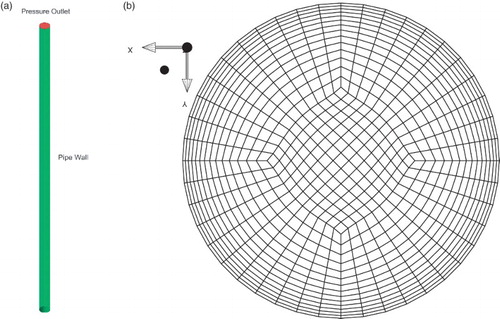
A 3D model of the flow domain was constructed using ANSYS ICEM-CFD Computer-Aided Design and meshing software. The flow domain is a vertical cylinder of height 9.5 m and with an internal diameter D of 0.29 m (Figure 4(a)), with z=0 coincident with the base of the cylinder. Again using ICEM, a structured O-Grid mesh was created (Figure 4(b)). This choice of mesh permits a refinement normal to the pipe walls to resolve the film around the Taylor bubble and the Stokes boundary layer, whilst retaining a relatively coarse mesh near to the center of the pipe. The use of hexahedral meshes has been shown to deliver better quality simulations than tetrahedral meshes (Abdulkadir, Hernandez-Perez, and Azzopardi, 2011) and so have been adopted in the current study.

Figure 4. Details of the domain used in the simulations in section 4: (a) the domain and (b) an xy cross-section of the mesh. Note: The domain has a total height of 9.5 m and a diameter of 0.29 m; the mesh has a spacing of 0.0005 m at the wall rising to 0.0075 m at the center.

A series of preliminary studies were undertaken to evaluate the level of error introduced by the numerical modeling. There are multiple potential sources of error in a CFD simulation which must be minimized. These errors fall into the following categories: errors in the physical modeling of the problem, discretization errors, errors in the CFD code and computational round-off errors. To ensure minimal discretization errors in the spatial domain, a grid convergence study was undertaken on the computation of the rise velocity of the bubble by using the Grid Convergence Index (GCI) method of Roache (1998). Temporal convergence was computed in a similar manner. The application of the GCI method concluded that the error introduced by spatial discretization was found to be 0.411% at an average vertical grid spacing of 0.008 m, with a spacing at the wall of 0.0025 m rising to 0.0075 m, and temporal discretization to be 0.175% using a time step of 0.0005 s.

The results produced by the chosen RKE model was compared to the experimental results presented in Pringle et al. (2015). The RKE model was found to under-predict the rise velocity of Taylor bubbles by approximately 17% with a Froude number of .

3.3. Initial and boundary conditions

A base case model was created, against which all further simulations except the validation of Appendix 1 were compared. In this base case, the model pipe was initially filled with water to a depth of 5 m, with 4.5 m of air above this. A bubble of air was then introduced close to the base of the pipe by specifying the volume fraction of air to be unity in an appropriate region. It is not essential to match the depth of water in the experiments (6 m) to the simulations, because it is the distance of the bubble from the top of the liquid column which is important for bubble dynamics (i.e., a simulated bubble 2 m from the top of a 5-m column of water behaves the same as a bubble 2 m from the top of a 6-m column).

The initial size and shape of the bubble was varied to represent the range of different laboratory experiments performed. The bubble's initial shape for the base case is that of a hemisphere attached to a cylinder with a radius of 0.14 m and a length of 0.5 m, giving a total length of 0.64 m. This is similar to the bubbles observed in the experiments of Taha and Cui (2004). The initial pressure in the bubble was set at a constant value matching the hydrostatic pressure at the nose of the bubble. Contour plots of the initial volume fraction and static pressure are shown in Figure 5. The initial velocity field was set to zero everywhere.

Figure 5. Contour plots of (a) the initial volume fraction (where red represents the air and blue represents the liquid), and (b) the initial gauge pressure after a hydrostatic distribution has been specified.

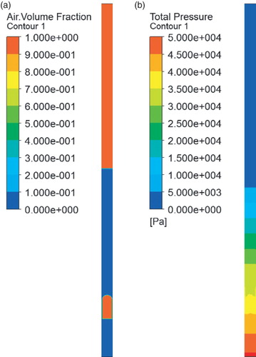
The reference pressure was set as atmospheric pressure (101,325 Pa) and specified at a location which was always within the gas phase above the upper liquid surface. The water surface level was tracked by a user-defined function (UDF) which determines the maximum level of the water surface at each time step.

4. Results

4.1. Bubble rise

In the base case, the Taylor bubble was initialized with a pressure equal to the hydrostatic pressure at its nose. This is akin to a slow injection of gas at the base of the pipe in the experiment, followed by a very gradual shut off of the valves. In the experimental study, this produced the formation and rise of a Taylor bubble with no noticeable oscillations observed during its ascent. The solution from the CFD model for this case replicates the expected behavior – a stable Taylor bubble is produced and the liquid surface rises at a constant rate until a rapid expansion of the bubble is observed as it approaches the surface, which can be seen in the middle line of Figure 6. This effect has been previously noted for Taylor bubbles in pipes that are 0.025 m in diameter (James et al., 2008).

Figure 6. Variation of water surface height over time for various initial pressures in the bubble in intervals of 10 kPa, ranging from a 30 kPa under-pressure (lowest line) to a 30 kPa over-pressure (highest line). Note: The central line is for a bubble initialized at the hydrostatic pressure.

Since an isothermal, ideal gas model is being used, given an initial hydrostatic pressure distribution, for a bubble of initial volume 0.0365 m³, with its nose at a depth of 3.36 m, the surface would be expected to rise by 0.168 m due to the expansion of the bubble. This closely matches the value of surface rise of 0.170 m from the numerical simulation (Figure 6). As the pressure is specified at the nose of the bubble, this is slightly below the actual pressure in the bubble because of the complex way in which the hydrostatic pressure varies around the hemispherical nose region of the bubble. This causes a small initial under-pressure which results in relatively small oscillations, even for a bubble that is meant to have an internal pressure equal to the hydrostatic pressure. Further, no increase in the bubble length is observed, as any expansion due to reduced hydrostatic pressure is offset by the loss of small bubbles into the wake region. Indeed, the mean length of the bubble is seen to increase by no more than 5% in these simulations.

Due to the oscillatory nature of the bubble rise, a continuous tracking of the bubble position is required to compute the rise velocity accurately. A comparative analysis of the theoretical predictions and experimental results suggests a non-dimensional rise rate of . However, the base case CFD model simulation computed a lower value of . At higher Froude numbers, previous CFD studies have also displayed a similar under-prediction of the rise velocity (James et al., 2008). Indeed, as is discussed in Appendix 1, this difference is due to the inability of the RANS model to accurately predict the turbulent flow in the falling film. Experimental measurements were taken at the nose of the bubble, as the position of the base of the bubble is difficult to track continuously due to the shedding of smaller bubbles. Estimates of this base velocity were recorded and found to be comparable to the nose velocity, with the exception of the rapid expansion as the bubble approaches the liquid surface.

4.2. Oscillating bubbles

In the experimental studies, the initial pressure inside the bubble is influenced by the method used to shut off the air injection tap. An analysis was carried out with the numerical model to investigate the effect of varying the initial pressure inside the bubble. An initial pressure inside the bubble that is above the hydrostatic pressure means that the bubble is initially compressed, so it tends to expand before contracting again, and then expand once more as it enters an oscillatory mode. Conversely, an initial pressure below the hydrostatic pressure means that the bubble has a larger length than it would have under stationary hydrostatic conditions, and thus it tends to compress. The magnitude of the difference from the hydrostatic pressure determines the amplitude of the resultant oscillations. An initial bubble length of 0.64 m with the nose at z=1.64 m and a depth of water 5 m were used in this part of the investigation.

If the first peak in surface height (Figure 6) is considered for an initial over-pressure, the amplitude of the surface height oscillations appears to scale linearly with the pressure disturbance. With a 10 kPa over-pressure, a surface height rise of approximately 0.07 m is seen, then with 20 kPa it is 0.13 m and with 30 kPa it is 0.21 m. A similar trend can be observed for the under-pressure cases, although the magnitude of the surface oscillations is smaller. Whilst the over- and under-pressure cases are initially out of phase by , this is not maintained throughout the bubble rise, since the frequency of oscillation is a function of the height of the water column H, and so the phase of the oscillation is observed to shift in a non-trivial fashion.

In Figure 6, the bubble at an initial 30 kPa under-pressure is observed to burst slightly sooner than in the other cases. This is due to the bubble breaking up shortly after the start of the simulation. The several smaller bubbles into which it breaks rise faster than the single bubble would, which results in an apparent acceleration in the first 0.5 s of the simulation. After 1 s, the bubble is observed to reform and follows the same rise rate as the other cases for the remainder of its progress. The frequency of the oscillation determined for the reformed bubble is not significantly altered by this initial breakage and recombination phase. This is the only case in which an instability (due to the under-pressure) is observed to cause the bubble to break, and once the bubble recombines, it remains stable for the rest of the rise. Incidentally, had such behavior been observed in the initial stages of bubble rise in the experimental study, the bubble would have been regarded as stable because stability was not evaluated until it had traveled 3 m from the base of the pipe.

Figure 7(a) shows the variation of water surface height for the CFD simulation and analytical model for the case with a 20 kPa overpressure. For the CFD simulations, the peaks of the water column surface height were extracted using the MATLAB findpeaks function and frequencies were calculated from the inverse of the peak-to-peak time. A similar process was performed by Pringle et al. (2015) in the calculation of the frequency in the experiments. Initially, there is good agreement between the analytical model and the CFD for the first complete oscillation but, as is discussed in the next paragraph, the frequency of oscillation differs between the two and they quickly move out of phase with each other. However, over the first period of the bubble rise, the mean surface level is predicted to rise in a consistent manner for the two models. The divergence toward the end of the transit can be explained by the fact that the analytical model retains the air in the bubble, while the CFD model sheds bubbles in its wake. These smaller bubbles rise more slowly and hence do not expand at the same rate as the main bubble, resulting in a lower rise rate for the CFD predictions.

Figure 7. Plots for a bubble 0.64 m in length with a 20 kPa over-pressure of (a) the surface height for the CFD simulation (with peaks highlighted) and the analytical model and (b) the frequency of the surface oscillations for the CFD simulation, the experiment and the model.

The frequency of surface height variation is shown in Figure 7(b). The analytical model is a continuous curve, while the CFD and experimental results are discrete points for the reasons just given. The frequency of oscillation obtained from the CFD simulations is approximately 10% larger than the experimental value during the early stages of the rise (Figure 7(b)). The CFD predictions do not quite fall within the upper error bound of the experimental results. The error bars associated with the experimental results are found by assuming a binomial distribution across the ten repeated experiments and represent 1 standard deviation from the mean value. The analytical model solutions more closely replicate the observed experimental behavior compared to those of the corresponding CFD models, but both clearly diverge from the experimental frequency as the surface is approached. For the analytical model, this may have been expected because none of the complex behavior of the flow in the liquid ahead of the bubble is included in the model. For the CFD model it is more surprising because much of the flow physics in the nose region is modeled and, as has been shown, is modeled well.

The gauge pressure was determined from the numerical simulations using a monitor located on the pipe wall at a height of 1.5 m above the base of the pipe. So, initially the monitor point is level with the bottom of the hemispherical cap of the bubble. In Figure 8, where there is an initial over-pressure of 20 kPa and a water depth of 5 m, the pressure is π out of phase with the surface oscillations, with the pressure inside the gas bubble being at maximum when the water surface is at its lowest level. This is due to the compression of the bubble which increases the pressure inside it, which in turn increases the pressure within the adjacent liquid film. In the Figure 8, the pressure oscillates around a mean value of approximately 30 kPa gauge pressure, which is somewhat lower than the hydrostatic pressure at 3.5 m below the initial water level. This deficit can be explained by the presence of the bubble, 0.64 m in length, which does not contribute appreciably to the hydrostatic pressure.

Figure 8. Comparison between pressure oscillations and surface oscillations with an initial over-pressure of 20 kPa. Note: The pressure at a height of 1.5 m on the pipe wall is indicated by the heavy line and the location of the surface by the lighter line. The maximum pressure in the fluid corresponds to the minimum surface height and thus to the maximum compression of the bubble.

4.3. Variation of bubble length

The initial length of the Taylor bubble, , was varied across a range of values from 0.29 m to 1.04 m (D to 3.5D). In the models of Pringle et al. (2015), Vergniolle et al. (1996) and section 2 of the present study the frequency is proportional to . This relationship is confirmed to some extent by an analysis of the experimental studies. However, as only two initial bubble lengths have been investigated, firm conclusions cannot be drawn. In a subsequent analysis of CFD simulations in which many more initial lengths were modeled, good agreement is observed – as demonstrated in Figure 9, where frequency is plotted against at specific times in the rise of the bubble.

Figure 9. Frequency of the surface oscillations plotted against for bubbles of initial length ranging from 0.28 m to 1.04 m at various times prior to bursting through the water surface.

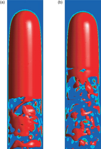
In section 4.2, it is proposed that the variation in frequency due to changes in the initial pressure is caused by variation in the lengths of the bubbles created. The average lengths (i.e., the length of the bubble at hydrostatic equilibrium) range from 0.70 m for the 30 kPa over-pressure case to 0.44 m for the 30 kPa under-pressure case. The differences in bubble length for these two cases can be seen in Figure 10. In the figure, the shedding of smaller bubbles can be seen behind the main bubble. The resolution of the mesh used is such that only bubbles above a certain size can be resolved. Since these shed bubbles are responsible for a loss of volume in the main bubble, the correct modeling of them could impact on the simulation. Despite these lost bubbles, for each simulation, L increases as the bubble rises up to the water surface. Plotting versus time to burst (not included for brevity) shows that all the data collapse onto a single curve, confirming that the average bubble length controls the oscillation frequency. These simulations demonstrate that the numerical model is capable of replicating the experimental behavior for a range of bubble lengths. For all bubble lengths investigated, the Taylor bubble remained stable, as in the base case.

Figure 10. Taylor bubble with (a) 30 kPa over-pressure and (b) 30 kPa under-pressure.

4.4. Stokes boundary layer

In section 2, the model includes a viscous damping term that was hypothesized to be due to the presence of a very thin Stokes boundary layer caused by the vertical oscillation of the plug of water ahead of the Taylor bubble. In the air–water bubble system, the damping caused by the presence of the Stokes boundary layer is negligible, but it is proposed that a Stokes boundary layer should exist because the Womersley number α is greater than 10. Figure 11 shows the w-component of the liquid velocity at a series of points close to the wall of a CFD simulation (denoted by the circular symbols) at a location ahead of the bubble at various times during a single expansion/compression cycle of an oscillating Taylor bubble. Because the bubble is rising, the plots are not symmetrical but do show that an oscillating boundary layer is formed. Indeed, using the MATLAB function nlinfit, it is possible to fit a curve of the form of Equation (8(8) ) through each set of points to produce instantaneous values of , Ω and κ. Since the depth δ of the Stokes boundary layer is given by (31) it was found that the value of δ varies between 2.8 mm and 4.1 mm during the oscillation cycle. This confirms that the Stokes boundary layer is present and that outside of this region the fluid behaves like a plug (as witnessed by the flat velocity profiles in Figure 11). Further, Figure 12(a) shows the variation of the wall shear stress with time at some height on the wall, well ahead of the bubble, while Figure 12(b) shows the w-component of the water velocity at the same height, but well outside the Stokes boundary layer. Equation (11(10) ) predicts a phase difference between these two variables of . In fact, the CFD model predicts a phase difference of approximately , which may be due to the presence of the hemispherical cap of the Taylor bubble, which creates some additional variation in the w-component of the velocity in the wall-normal direction.

Figure 11. Plots of the w-component of velocity against the wall-normal coordinate y at a constant value of z ahead of a rising Taylor bubble at various points during an expansion/contraction cycle. Note: The solid lines show fits through the data points.

Figure 12. The variation with time of (a) the wall shear stress at a point on the wall above the rising Taylor bubble and (b) the w-component of the velocity at the same height and well outside of the Stokes boundary layer.

4.5. Variation of liquid viscosity

Vergniolle et al. (1996) suggest that one of the causes of the acoustic variations measured at volcanic sites could be Taylor bubble oscillations. Magma is several orders of magnitude more viscous than water, and therefore it was deemed reasonable to test the predictions of the CFD model as the viscosity was so increased. The values of viscosity modeled range from the 0.001 Pa s of air to 45 Pa s, which is typical of volcanic magma.

Viana et al. (2003), after analyzing data from numerous experiments on Taylor bubbles in the literature, developed a ‘universal’ correlation between Fr and R, the buoyancy Reynolds number: (32) where g is acceleration due to gravity and the and subscripts refer to the liquid and gas phases, respectively. The buoyancy Reynolds number is the square root of the Archimedes number. Viana et al. (2003) demonstrated that there are three regimes: when , in which Fr is independent of R and where inertial forces dominate; when , where viscous forces dominate and R is a function of Fr (and Eo); and a transition regime, which is more complex.

In the CFD simulations, the range of viscosities investigated correspond to a variation in the buoyancy Reynolds number from 10 to . For those simulations with , it was found that there is very little change in the Froude number over a wide range of R (a decrease of 4% from to 600). However, in the transition regime, Froude numbers of 0.243 and 0.122 are observed at buoyancy Reynolds numbers of 50 and 10, respectively, which is consistent with the findings of Viana et al. (2003).

For the range of liquid viscosities considered, where R is in the inertial range, an increase in the viscosity does not appear to significantly affect the bubble oscillation frequency (Figure 13). This figure is constructed by determining the instantaneous frequency of oscillation for various bubbles in fluids of different viscosity at various times prior to bursting through the surface. The independence of the frequency from the viscosity is also in agreement with the form of the model presented in section 2, where is independent of the viscosity (Equation (14(13) )).

Figure 13. Frequency of bubble oscillations for liquids of varying viscosity for buoyancy Reynolds numbers ranging from 600 to 500,000.

However, the amplitude of the oscillations is clearly dependent on the viscosity, as can be seen in Figure 14, which shows the first three oscillations of the liquid surface. Despite the lack of a key, the peaks decrease with increasing viscosity and hence damping. Because the peak height decreases as the bubble rises, it is problematic to disentangle this phenomenon from that of the effect of viscous damping on the peak height. However, if only the first peak in Figure 14 is considered, it is possible to test the predictions of the analytical model. For an under-damped case, the general solution to Equation (13(12) ) is (33) where and are the undamped and damped natural frequencies, respectively. Hence, from an analysis of Equation (15(14) ) for Womersley numbers greater than 10, it might be expected that the first peak rise be proportional to .

Figure 14. The first three oscillations of the surface for liquids of varying viscosity for buoyancy Reynolds numbers ranging from 60 to 500,000.

Figure 15 shows a plot of the first peak rise against for buoyancy Reynolds numbers from 60 to . The viscosity of the fluid decreases from left to right. There appear to be two distinct regions, three points in the low viscosity, high Reynolds number range, and five points in the higher viscosity, lower Reynolds number range. In fact, the three leftmost points correspond to both R<200 and a Womersley number of , which correspond to the point at which the flow is transitioning from inertial to viscous. Hence, it is difficult to draw any conclusions from this plot, other than that there is a clear trend – the first peak rise predicted by the CFD simulation reduces as the viscosity increases, which would be expected.

Figure 15. A plot of the surface rise for the first peak in Figure 14 against for various liquids for buoyancy Reynolds numbers ranging from 60 to 500,000.

4.6. Flow fields

The flow field around the rising Taylor bubbles in an air–water system was assessed at various points in the flow domain during a typical oscillation. When in compression there is a small positive, vertical component of velocity ahead of the bubble for a length of approximately D/8 (Figure 16(a)). In this case, the bubble is still moving upwards, despite being in the compression phase. The streamlines indicate that the liquid bypasses the nose region and continues down into the film region around the bubble. This behavior is similar to the particle image velocimetry (PIV) results published in the literature (van Hout et al., 2002; Nogueira et al., 2006b), with clear variations observed due to the oscillatory behavior and differing rise velocity of the bubble.

Figure 16. Streamlines (left) and velocity vectors (right) for a Taylor bubble: (a) around the nose whilst compressing, (b) around the nose while expanding, (c) in the wake whilst compressing, and (d) in the wake whilst expanding.

During the expansion phase of the oscillation (Figure 16(b)), all of the water ahead of the bubble is forced upwards, causing the surface to rise. Some of the flow is washed down the side of the bubble into the liquid film, which then enters the wake behind the bubble. The wake behind the bubble is open both in compression and expansion, as opposed to an attached wake region behind the bubble observed in laminar flows (Figure 16(c) and (d)). This phenomenon is due to the large Eo number caused by the large pipe diameter in relation to the low-viscosity fluid used.

5. Conclusions

In this paper, it has been demonstrated that a great deal can be learnt about the behavior of oscillating Taylor bubbles rising in a quiescent liquid through the use of URANS CFD simulations. Numerical modeling of this type allows many physical (and unphysical) situations to be modeled quickly and accurately, using parameter sets that are simply impractical in the laboratory. However, the validation of such models is key, and the experimental work of Pringle et al. (2015) has proved invaluable in providing an indication of the accuracy of the numerical modeling. In addition, the adaption and improvement of the analytical model proposed by Pringle et al. (2015) to include damping via the Stokes boundary layer has given yet more insights into the role of the plug of liquid ahead of the rising bubble.

Key to the success of the modeling approach is the use of a compressible gas and the application of initial over- and under-pressures, which instigate the oscillations in the rising bubble and the resultant movements in the liquid surface. However, without initial pressure perturbations, stable Taylor bubbles were successfully simulated with a rise rate within 18% of the experimental values. For these stable cases, the liquid surface rise level is within 5% of the predicted values. For the oscillating cases, the predicted numerical frequencies are within 10% of the experimental values and display similar behavior to the analytical model. This agreement is strong in the early stages of the bubble rise, but as the bubble approaches the surface, both the CFD model and the analytical model diverge from the experimental observations. It is concluded that the plug-flow assumption of the analytical model may break down as the spherical nose of the bubble makes a greater proportion of the liquid column height near the surface. With the CFD modeling, the divergence can perhaps be explained by the URANS simulations artificially producing a turbulent viscosity, which differs from the true flow physics as the bubble approaches the surface. Alternatively, the wake region is not modeled well by the URANS model and the shedding of gas from the bubble may be less pronounced in the experiments. Since the frequency of oscillation is proportional to , if the numerical bubble loses more gas (in the form of small bubbles shed in the wake) then the frequency may be observed to increase artificially quickly.

The incorporation of the damping term into the analytical model led to the investigation of the flow in the near-wall region ahead of the rising bubble. An analysis of the CFD solutions was able to confirm the presence of a Stokes boundary layer and add credibility to the inclusion of this term in the analytical model. The effects produced by a decrease in the buoyancy Reynolds number, by increasing the liquid viscosity, were studied using the numerical model and insights into applicability of the Stokes boundary layer were gained.

Acknowledgements

The authors would like to acknowledge the use of the High Performance Computer at the University of Nottingham.

Disclosure statement

No potential conflict of interest was reported by the authors.

Additional information

Funding

We would like to thank the NERC for funding this research [grant number NE/G016593/1].

Appendix 1. Validation at a reduced scale

A validation study on a pipe with a smaller diameter than that of Pringle et al. (2015) was conducted to confirm that the model is capable of reproducing key flow characteristics. The solutions from the numerical model were compared against the experimental studies of van Hout et al. (2002), who used PIV methods to investigate the flow around a single Taylor bubble rising in stagnant water. The diameter of the pipe used in these experiments was 0.025 m, which results in the dimensionless numbers , and .

Qualitatively, the numerical solutions compare well to the experimental data in all respects. In particular, the flow field around the nose of the bubble and the behavior of the wake are very similar (Figure 17). The PIV results were averaged over 100 experimental runs to give the velocity field, whilst that determined from the CFD simulation is instantaneous and results from a single simulation. This is because the CFD simulations are deterministic and, using the same initial conditions, another run should produce the same result at that instant in time.

Figure A.1. Velocity vectors around a fully developed Taylor bubble. The plots on the left are for PIV results averaged over 100 Taylor bubbles (van Hout et al., 2002). The plots on the right are instantaneous results from a CFD simulation. In the top row the results are for a window from D/2 below the nose of the bubble to D/2 above it; the middle row is from 2D behind the tail of the bubble to the tail; the bottom row is from 4D to 2D below the tail of the bubble.

The axial velocity profiles within the liquid film region surrounding the Taylor bubble are shown in Figure 18, adjusted by position. This adjustment, proposed by van Hout et al. (2002), offsets the velocity by the position z at which it was recorded. This is such that a measurement read at with a downward velocity of 1 ms⁻¹ gives a reading of  ms⁻¹, where is at the nose of the bubble.

Figure A.2. Comparison of the outlines of the bubbles and velocity measurements adjusted by position for the experimental measurements in van Hout et al. (2002) and the CFD validation case.

Figure A.3. Comparison of the centerline velocity behind the tail of the bubble for the experimental measurements of van Hout et al. (2002) and the CFD validation case.

The outline of the Taylor bubble is also shown in Figure 18. At the entrance to the film at the top of the bubble the velocities are small, but as the film thickness decreases, the liquid is observed to accelerate, by conservation of mass. The velocity reaches a maximum value of approximately 1 ms⁻¹, close to the exit of the liquid film at the base of the bubble. The film Reynolds number Re for this case is given by (A1) where Q is the volumetric flow rate in the falling film, is the mean velocity across the film, δ is the film thickness, and R is the internal radius of the pipe. With estimated as 1 ms⁻¹, the film Reynolds number is 2100, indicating that the film is turbulent. The predicted maximum velocity in the film is 5% below the experimental value. The liquid film thickness of the simulations at the exit is 0.00114 m, as compared to 0.00117 m in the experiment, and it is this difference in film thickness that accounts for the discrepancy in the velocity of the film velocity. This then, through conservation of mass, has a knock-on effect, causing the simulated bubble rise velocity to be 5% lower than the experimental value. Thus, the difference may be due to the inability of the turbulence model or the law of the wall to model the turbulent flow in the film or because the wall-normal mesh resolution in the film region was inadequate.

It was also concluded that in the near wake region behind the tail of the bubble there are strong similarities in the flow behavior predicted by the numerical solutions and the experimental data (Figure 17, middle plots). Within two pipe diameters of the tail of the bubble, a strong vortex is observed. Near to the wall, the axial velocity profiles are similar to those of an annular jet. Figure 19 shows the centerline axial velocity behind the rising bubble. The peak of the positive axial velocity corresponds to the vertical flow where the two counter-rotating vortices meet immediately behind the bubble. Beyond this region, the centerline axial velocity reverses in direction, with a positive axial flow near the walls and a negative flow directed towards the central area, as can be observed in Figure 19 and, for the time-averaged experimental data, in the lower left plot of Figure 17.

References

- Abdulkadir, M., Hernandez-Perez, V., & Azzopardi, B. (2011). Grid generation issues in the CFD modeling of two-phase flow in a pipe. The Journal of Computational Multiphase Flows, 3(1), 242–252.
- ANSYS. (n.d.). ANSYS-FLUENT. Pittsburgh, PA: Ansys, Inc.
- Araujo, J. D. P., Miranda, J. M., Pinto, A. M. F. R., & Campos, J. B. L. M. (2012). Wide-ranging survey on the laminar flow of individual Taylor bubbles rising through stagnant Newtonian liquids. International Journal of Multiphase Flow, 43, 131–148. doi: 10.1016/j.ijmultiphaseflow.2012.03.007
- Brackbill, J. U., Kothe, D. B., & Zemach, C. (1992). A continuum method for modeling surface tension. Journal of Computational Physics, 100, 335–354. doi: 10.1016/0021-9991(92)90240-Y
- Brown, R. A. S. (1965). The mechanics of large gas bubbles in tubes. Canadian Journal of Chemical Engineering, 43, 217–223. doi: 10.1002/cjce.5450430501
- Davies, R. M., & Taylor, G. I. (1950). The mechanics of large bubbles rising through extended liquids and through liquids in tubes. Proceedings of the Royal Society of London A: Mathematical, Physical and Engineering Sciences, 200, 375–390. doi: 10.1098/rspa.1950.0023
- Dumitrescu, D. T. (1943). Strömung an einer Luftblase im Senkrechten Rohr. Zeitschrift für Angewandte Mathematik and Mechanik, 23(3), 139–149. doi: 10.1002/zamm.19430230303
- Ghosh, S., Patil, P., Mishra, S. C., Das, A. K., & Das, P. K. (2012). 3-d lattice Boltzmann model for asymmetric Taylor bubble and Taylor drop in inclined channel. Engineering Applications of Computational Fluid Mechanics, 6(3), 383–394. doi: 10.1080/19942060.2012.11015429
- Hayashi, K., Hosoda, S., Tryggvason, G., & Tomiyama, A. (2014). Effects of shape oscillation on mass transfer from a Taylor bubble. International Journal of Multiphase Flow, 58, 236–245. doi: 10.1016/j.ijmultiphaseflow.2013.09.009
- Hirt, C. W., & Nichols, B. D. (1981). Volume of fluid (VOF) method for the dynamics of free boundaries. Journal of Computational Physics, 39, 201–225. doi: 10.1016/0021-9991(81)90145-5
- James, M. R., Lane, S. J., Chouet, B., & Gilbert, J. S. (2004). Pressure changes associated with the ascent and bursting of gas slugs in liquid-filled vertical and inclined conduits. Journal of Volcanology and Geothermal Research, 129, 61–82. doi: 10.1016/S0377-0273(03)00232-4
- James, M. R., Lane, S. J., & Corder, S. B. (2008). Modelling the rapid near-surface expansion of gas slugs in low-viscosity magmas. Geological Society, London, Special Publications, 307, 147–167. doi: 10.1144/SP307.9
- James, M. R., Llewellin, E. W., & Lane, S. J. (2011). Comment on: It takes three to tango: 2. Bubble dynamics in basaltic volcanoes and ramifications for modeling normal Strombolian activity. Journal of Geophysical Research, 116, 1–5. Article no. B06207.
- Kang, C. W., Quan, S., & Lou, J. (2010). Numerical study of a Taylor bubble rising in stagnant liquids. Physical Review E, 81. doi: 10.1103/PhysRevE.81.066308.
- Ku, D. N. (1997). Blood flow in arteries. Annual Review of Fluid Mechanics, 29(1), 399–434. doi: 10.1146/annurev.fluid.29.1.399
- Lu, X., & Prosperetti, A. (2009). A numerical study of Taylor bubbles. Industrial and Engineering Chemistry Research, 48(1), 242–252. doi: 10.1021/ie800201x
- Marschall, H., Hinrichsen, O., & Polifke, W. (2008). Numerische Simulation von Mehrphasenreaktoren mittels hybridem CFD-Modell in OpenFOAM (HIRES-TFM). Chemie Ingenieur Technik, 80(9), 1303–1303. doi: 10.1002/cite.200750548
- MATLAB. (2012). MATLAB Release 2012a. Natick, MA: The Mathworks Inc.
- Ndinisa, N. V., Wiley, D. E., & Fletcher, D. F. (2005). Computational fluid dynamics simulations of Taylor bubbles in tubular membranes: Model validation and application to laminar flow systems. Chemical Engineering Research and Design, 83(1), 40–49. doi: 10.1205/cherd.03394
- Nogueira, S., Riethmuler, M. L., Campos, J. B. L. M., & Pinto, A. M. F. R. (2006a). Flow in the nose region and annular film around a Taylor bubble rising through vertical columns of stagnant and flowing Newtonian liquids. Chemical Engineering Science, 61(2), 845–857. doi: 10.1016/j.ces.2005.07.038
- Nogueira, S., Riethmuller, M. L., Campos, J. B. L. M., & Pinto, A. M. F. R. (2006b). Flow patterns in the wake of a Taylor bubble rising through vertical columns of stagnant and flowing Newtonian liquids: An experimental study. Chemical Engineering Science, 61, 7199–7212. doi: 10.1016/j.ces.2006.08.002
- Oguz, H. N., & Prosperetti, A. (1998). The natural frequency of oscillation of gas bubbles in tubes. The Journal of the Acoustical Society of America, 103(6), 3301–3308. doi: 10.1121/1.423043
- Parfitt, E. A. (2004). A discussion of the mechanisms of explosive basaltic eruptions. Journal of Volcanology and Geothermal Research, 134, 77–107. doi: 10.1016/j.jvolgeores.2004.01.002
- Polonsky, S., Barnea, D., & Shemer, L. (1999). Averaged and time-dependent characteristics of the motion of an elongated bubble in a vertical pipe. International Journal of Multiphase Flow, 25(5), 795–812. doi: 10.1016/S0301-9322(98)00066-4
- Pringle, C. C. T., Ambrose, S., Azzopardi, B. J., & Rust, A. C. (2015). The existence and behaviour of large diameter Taylor bubbles. International Journal of Multiphase Flow, 72, 318–323. doi: 10.1016/j.ijmultiphaseflow.2014.04.006
- Roache, P. (1998). Verification and validation in computational science and engineering. Albuquerque, NM: Hermosa.
- Sawko, R., & Thompson, C. (2010). Estimation of rate of strain magnitude and average viscosity in turbulent flow of shear thinning and yield stress fluids. International Conference of Numerical Analysis and Applied Mathematics.
- Shih, T.-H., Liou, W. W., Shabbir, A., Yang, Z., & Zhu, J. (1995). A new eddy viscosity model for high Reynolds number turbulent flows. Computers and Fluids, 24(3), 227–238. doi: 10.1016/0045-7930(94)00032-T
- Suckale, J., Nave, J.-C., & Hager, B. H. (2010). It takes three to tango: 1. Simulating buoyancy-driven flow in the presence of large viscosity contrasts. Journal of Geophysical Research, 115, 1–16. Article no. B07409.
- Taha, T., & Cui, Z. F. (2004). Hydrodynamics of slug flow inside capillaries. Chemical Engineering Science, 59, 1181–1190. doi: 10.1016/j.ces.2003.10.025
- van Hout, R., Gulitski, A., Barnea, D., & Shemer, L. (2002). Experimental investigation of the velocity field induced by a Taylor bubble rising in stagnant water. International Journal of Multiphase Flow, 28, 579–596. doi: 10.1016/S0301-9322(01)00082-9
- Vergniolle, S., Brandeis, G., & Mareschal, J.-C. (1996). Strombolian explosions: 2. Eruption dynamics determined from acoustic measurements. Journal of Geophysical Research: Solid Earth, 101(9), 20449–20466. doi: 10.1029/96JB01925
- Viana, F., Pardo, R., Yanez, R., Trallero, J. L., & Joseph, D. D. (2003). Universal correlation for the rise velocity of long gas bubbles in round pipes. Journal of Fluid Mechanics, 494, 379–398. doi: 10.1017/S0022112003006165
- White, E. T., & Beardmore, R. H. (1962). The velocity of rise of single cylindrical air bubbles through liquids contained in vertical tubes. Chemical Engineering Science, 17, 351–361. doi: 10.1016/0009-2509(62)80036-0
- Womersley, J. R. (1955). Method for the calculation of velocity, rate of flow and viscous drag in arteries when the pressure gradient is known. The Journal of Physiology, 127(3), 553–563. doi: 10.1113/jphysiol.1955.sp005276
- Yan, K., Zhang, Y., & Che, D. (2012). Experimental study on near wall transport characteristics of slug flow in a vertical pipe. Heat and Mass Transfer, 48(7), 1193–1205. doi: 10.1007/s00231-012-0969-y
- Yang, Z. L., Palm, B., & Sehgal, B. R. (2002). Numerical simulation of bubbly two-phase flow in a narrow channel. International Journal of Heat and Mass Transfer, 45(3), 631–639. doi: 10.1016/S0017-9310(01)00179-X
- Youngs, D. (1982). Time-dependent multi-material flow with large fluid distortion. Numerical methods for fluid dynamics (p. 273). New York: Academic Press.