Numerical study on surface distributed vortex-induced force on a flat-steel-box girder

ABSTRACT

To ensure the safety of bridges, the comfort of pedestrians and vehicles on bridges, the vortex-induced forces on flat-steel-box girders need to be investigated. The total vortex-induced forces integrated on the surfaces of girders have been studied extensively. This study will be mainly focused on the characteristics of surface distributed vortex-induced force, which can be beneficial to the vortex-induced vibration (VIV) reduction with local aerodynamic optimization. Computational Fluid Dynamics (CFD) method is employed for the simulation of the VIVof a flat-steel-box girder. The simulation results are verified through the comparison with the results of corresponding wind tunnel test. A self-adaptive nonlinear fitting method is proposed to determine the vortex-induced force model. A vortex-induced force contribution factor is defined to account the contribution of the components and the surface location. Based on the surface distributed vortex-induced force analysis, several conclusions are made. The vortex-induced force presents a fairly strong multiple-frequency characteristic, and the high-order terms should be carefully considered. Most energy of the VIV comes from the linear and third-order aerodynamic damping terms. In terms of location, the roof takes most of the aerodynamic damping and the total vortex-induced force. The flow separation around the underside upstream corner, the underside downstream corner and the middle downstream comer lead to large third-order aerodynamic damping term. The flow separation around the underside upstream corner has great contribution to the linear aerodynamic stiffness term.

KEYWORDS:

• Flat-steel-box girder
• numerical simulation
• vortex-induced vibration
• vortex-induced force
• self-adaptive nonlinear fitting
• surface distribution and contribution

1. Introduction

Flat-steel-box girders are widely adopted in long-span bridges, for the advantages of light weight, high strength and good aerodynamic performance against flutter instability. Nevertheless, this kind of girder is often subjected to vortex-induced vibration (VIV) at low wind speeds, such as Storebelt Bridge (Larsen, Esdahl, Andersen, & Vejrum, 2000), Trans-Tokyo Bay Crossing Bridge (Fujino & Yoshida, 2002) and Xihoumen Bridge (Laima, Li, Chen, & Li, 2013; Li et al., 2011). Although VIV is a kind of self-limited vibration without disastrous consequences, continual VIVs may cause structural fatigue and discomfort to pedestrians and vehicles. Thus, VIV of flat-steel-box girders should be taken seriously, and an accurate and reasonable prediction is necessary.

It should be noted that most efforts have been focused on the VIVs of circular cylinders, which are easier to reveal some fundamental mechanisms. A large number of studies adopting wind tunnel tests are contained in several reviews, such as Williamson and Govardhan (2004), Sumner (2010), Bearman (2011) and Wu, Ge, and Hong (2012). And relative full-scale researches of CFD of circular sections are presented at the early twenty-first century (Guilmineau & Queutey, 2002; Kumar & Dalal, 2006; Tamura, 1999). In fact, compared with circular cylinder, VIV of non-circular section has different characteristics. However, limited research can be found for non-circular sections, especially for the flat-steel-box bridge decks. The experimental results of Diana, Resta, Belloli, and Rocchi (2006) indicated significant nonlinear behaviors of the vortex-induced force on a multi-box deck. Sun, Owen, and Wright (2009) testified that 2D simulation with k-ω RANS turbulence model is appropriate to simulate the wind-induced forces on bluff bodies compared with the 3D simulation. The mechanism and vibration reduction of VIV of a box cross section in the presence of aerodynamic countermeasures were discussed by Sarwar and Ishihara (2010), which showed the influences of fairings and flaps. Hallak et al. (2013) discussed the aerodynamic behavior of a girder in the presence of tall vehicles via 2D CFD model. Section and full aero-elastic model experiments of VIV were conducted and the differences between the two testing results were discussed by Sun, Li, and Liao (2013). However, the mechanism of nonlinear vortex-induced vertical force at resonance stability period on flat-steel-box bridge deck has not been studied extensively.

After lots of exploration about the principles and phenomena of the VIV, only a few researchers proposed mathematical models which are suitable for long-span bridges (Ehsan & Scanlan, 1990; Larsen, 1995; Scanlan, 1981; Simiu & Scanlan,1996). However, these models cannot reflect the features of vortex-induced force comprehensively, and the traditional identification methods introduced in those studies cannot identify precise model parameters to reconstitute the displacement response which could agree well with the CFD results. Aimed at the defects of Scanlan’s model and traditional parameters identification method, lots of efforts have been made and some new opinions have been proposed (Meng, 2013; Zhu, Meng, & Guo, 2013). They predicted the responses of flat closed-box cross sections using Scalan’s model, and it was found that this model was not appropriate for flat closed-box sections. Afterwards, a new nonlinear model of vortex-induced force for flat closed-box deck, which could reconstitute the vortex-induced force more precisely, was proposed by Zhu et al. (2013). Wind tunnel tests were adopted in the studies mentioned above, which might be influenced by many unpredictable factors, even the results might differ from each other at different wind tunnels with the same research targets (Sarkar, Caracoglia, Haan, Sato, & Murakoshi, 2009). With the development of the computational techniques, numerical simulation gradually becomes a powerful tool to investigate the VIV of bridges, for its convenience and quickness.

In this study, CFD was utilized to explore the vortex-induced force of a flat-steel-box girder. In Section 2, the simulation method and numerical model were introduced firstly. The results obtained from CFD including both the displacement and the vortex-induced force were then compared with those in wind tunnel test in Section 3, to validate the accuracy of the numerical simulation method. In Section 4, a Self-adaptive Nonlinear Fitting Method (SANFM) was introduced, in order to establish an appropriate mathematical model for vortex-induced force of the flat-steel-box girder. The corresponding model was compared with an advanced vortex-induced force model proposed in Zhu et al. (2013). Based on SANFM, the vortex-induced force model of the flat-steel-box girder from the CFD results was then obtained. A contribution factor based on energy spectrum was defined, and the contributions of vortex-induced force components and the locations on the girder to total vortex-induced force were analyzed in Section 5. Finally, some conclusions of this study were drawn in Section 6.

2. Numerical simulation

2.1. Simulation scheme

The flows around the girder should be simulated to obtain the vortex-induced force. The governing equations of incompressible viscous fluid include mass conservation equation (continuity equation), momentum conservation equation (Navier-Stokes equation) and energy conservation equation. For the air flow around the girder, the heat flux is very limited, thus the energy equation is ignored when calculating VIV responses. After being Reynolds averaged, the governing equations become (1) (2) where and are the density and the dynamic viscosity coefficient of air, respectively; subscript i, j represent the coordinate axis in space with i = 1, 2 and j = 1, 2 for two-dimensional simulation; x_i is the coordinate value along the i axis; and are the average velocity and the fluctuating velocity along j axis, respectively; t is the time; p is the pressure; and is the so-called Reynolds stress. In this study, the commercial software FLUENT was employed with SST k-ω turbulence model to model the Reynolds stress. Second-order scheme was used to discretize the governing equations, based on the finite volume method. SIMPLEC algorithm was employed for the pressure-velocity coupling. The least squares cell-based method was utilized for the gradient term. The pressure was discretized in a standard way. The momentum, turbulent kinetic energy and specific dissipation rate were discretized in second-order form. The above scheme was applied effectively in Wang, Xu, Zhu, Cao, and Li (2013).

2.2. Computational domain, boundary conditions and meshing

A flat-steel-box girder of a real long-span bridge is taken as an object, and the wind tunnel test results have been discussed in Zhu et al. (2013). The Wind tunnel tests were carried out in the TJ-3 boundary layer wind tunnel. This wind tunnel is 15 m wide, 2 m high and 14 m long. The turbulence intensity is less than 2.5%. For the sectional model, the scale ratio is 1:20, and the model length is 3.6 m. Moreover, an improved force measurement technique for vortex-induced force (VIF) was adopted in the wind tunnel tests. In order to validate the numerical simulation, the wind attack angle, wind speed and scale ratio in this study are set as the same as these in the wind tunnel tests. That is: the wind attack angle is+5°, the wind speed is 9.1 m/s, and the scale ratio is 1:20. The corresponding Reynolds number is 1.06 × 10⁵ based on the height of the girder.

The computational domain is shown in Figure 1. B and D are the width and the depth of the scaled girder, respectively. The width and the depth of the whole computational domain are 17B and 28D, respectively, with a blocking rate of 3.57%. The computational domain is divided into Rigid Domain, Dynamic-Mesh Domain and Stationary Domain as in Huang, Liao, Wang, and Li (2009). Rigid Domain has a rectangle area of 1.12B × 1.25D. The distances from the left edge, right edge, upper edge and lower edge of this domain to the corresponding outermost edges of the girder are 0.05B, 0.1B, 0.125D and 0.125D, respectively. In order to ensure the grid quality near the deck, a body-fitted structured quadrilateral mesh with 15 boundary layers is generated in Rigid Domain. Along the deck, the grid sizes are arranged between 9.6 mm∼18.8 mm, with a majority of 10 mm, which is about 1/3200 of the total width of the girder. Around the railing, the grid sizes are near 10 mm, which is about 1/17.5 of the width of the railing. Around the track maintenance track, the grid sizes are about 4 mm, which is about 1/30 of the width of the maintenance track. The mesh in Dynamic-Mesh Domain is filled with triangular grids. This domain is 3B in width and 10D in height. Stationary Domain is extended from the Dynamic-Mesh Domain to the out boundaries. For the flow around the girder, a vortex street may appear at the downstream region behind the girder in Stationary Domain. The grids in this domain should be densified and identified as Wake Domain to simulate this phenomenon clearly. Wake Domain is a long-narrow quadrilateral of 9.5B × 10D, filled with square grids. Thus, Stationary Domain contains Wake Domain and Exterior Domain.

Figure 1. Computational domain sketch.

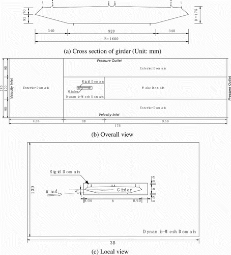
Figure 1 also shows the boundary conditions. The wind attack angle is produced by rotating the inlet flow while the girder keeps horizontal. The left out edge and the lower out edge are the sources of the wind, so they are defined as velocity inlets with a speed of 9.1 m/s. And a turbulent intensity of 0.02 and a turbulent viscosity ratio of 2 are assigned to them. After passing the computational domain, the wind flows out through the right out edge and upper out edge. Thus, the right edge and the upper edge are specified as pressure outlets with a gauge pressure of zero. The whole girder is defined as wall condition. In the whole domain among these boundaries, the flows are solved based on Eqs. (1-2).

2.3. Movement simulation of girder

Aerodynamic lift force is calculated through CFD and applied on the girder. The movement of the girder in the vertical direction is controlled by a basic dynamic equation as (3) where , and are the vertical displacement, velocity and acceleration of the girder at time t, respectively; m, c and k are the mass, mechanical damping coefficient and stiffness of the girder, respectively. m and k are converted from the parameters in the wind tunnel test of Zhu et al. (2013), which are 50.61 kg/m and 15742.76 N/m, respectively. Moreover, in order to improve the computational efficiency when verifying the independence of grid and time step, the damping coefficient is a constant of 8.926 N·s/m. Fourth-order Runge-Kutta method is used to solve Eq. (3) to obtain the responses of the girder at each time step. The vortex-induced force at the previous time step is applied approximately as . From the results in Section 3, this approximation can be accepted.

Dynamic mesh approach was utilized in this study according to Batina (1990) and Huang et al. (2009). Rigid Domain (see Figure 1) is linked with the girder and moves with it together. The grids in Dynamic-Mesh Domain are deformed at every time step. And the elastic smoothing method together with local remeshing method is applied to the deformation of the grids in Dynamic-Mesh Domain. When the deformation is very small, the elastic smoothing method is applied. The grid lines are similar to springs, any ending node moves elastically. The elastic rigidity of the two conterminous nodes i and j is (4) where x_i and x_j are the locations of node i and node j. The whole elastic force imposed on any node should be zero at any time, that is (5) where n_i is the number of the nodes near to node i. Thus, in Dynamic-Mesh Domain, the aforesaid equation can be defined as (6) where K is the elastic rigidity of this virtual spring between nodes; and is the displacement vector of the nodes.

When the deformation of the grids is relatively large, the elastic smoothing method is not applicable, but the local remeshing method, introduced in Fluent 6.3 user’s guide (2006), is applied. This method includes four steps. First, all the grids whose cell skewness or sizes exceed the formulary range are marked. Second, all the marked grids are deleted and empty cavities are formed around these grids. Thirdly, these empty cavities are reconstructed with new grids. The quality of the new grids is better than that of the marked grids. Finally, the values of these physical quantities on the new grids are interpolated from the former grids. The principle of the interpolation is to guarantee that the flow physical parameters are consistent before and after interpolation.

2.4. Independence study of grid and time step

Three time steps of 0.000223s, 0.000445s and 0.00089s are chosen to check the independence of the time step on the numerical results, corresponding to T/1600, T/800 and T/400, respectively (T is the natural vibration period of the girder). For each case, the results in the first 10 seconds are ignored, and the results in the following 10 seconds are chosen to be compared. Table 1 shows the computed results at different time steps. As can be seen from Table 1, the amplitude of the vertical displacement enlarges with the increase of the time step. And the Strouhal number reduces with the increase of time step. The results of the first two time steps (T/1600 and T/800) are somewhat similar. Compared with other time steps, it can be seen that the time step of 0.000445s is precise enough, thus, it is adopted in the following numerical simulation.

Table 1. Computed results with three different time steps.

Time step (s)	Amplitude of Vertical displacement (mm)	Vibration Frequency (Hz)	Strouhal number
0.000223	23.35	2.73	0.0525
0.000445	24.97	2.73	0.0525
0.00089	26.51	2.71	0.0521

In the process of the numerical simulation, the y⁺ value has great influence on the calculation results, which is decided by the height of the first layer grids. Consequently, as can be seen in Table 2, three meshing schemes with different heights of the first layer grids are created to check the independence of the numerical results on the grid sizes. G1 has the largest grid number of 0.35 million, the height and maximum y⁺ of its first layer grids are 0.0015 mm and 0.2, respectively. G2 increases the height of the first layer grids to 0.0075 mm, with 0.24 million grids. The maximum y⁺ value is 0.7. Its grid distribution is shown in Figure 2. G3 further increases the height of the first layer grids to 0.015 mm, and the maximum y⁺ value is 1.5, with 0.14 million grids. The computed results on different grids are shown in Table 2. The results of G1 are very close to those of G2, but the results of G3 are far away from those of G1 and G2. In consideration of both the precision of the numerical simulation and the computational efficiency, the meshing scheme G2 is finally applied to the following numerical simulation.

Figure 2. Grid distributions in meshing scheme G2.

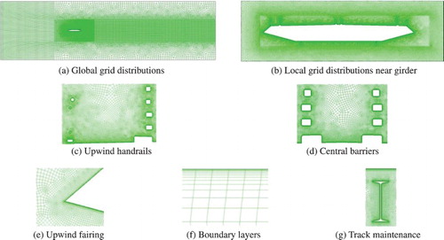
Table 2. Computed results with three different meshing schemes.

Meshing scheme	First layer grids height (mm)	Grid number (million)	Maximum y^+ value	Amplitude of Vertical displacement (mm)	Vibration Frequency (Hz)	Strouhal number
G1	0.03	0.35	0.2	33.47	2.75	0.0530
G2	0.15	0.24	0.7	33.52	2.76	0.0531
G3	0.3	0.14	1.5	24.97	2.73	0.0525

3. Simulation results and validation

In fact, the structural damping ratio may vary nonlinearly with the change of vibrating amplitude. Zhu et al. (2013) simplified the nonlinear variation of the structural damping ration with a linear equation: (7) where is the structural damping ratio; y is the vibrating amplitude. In this numerical study, the variation of structural damping is also taken into consideration.

It is hard to input the structural damping timely in the simulation due to the fact that the vibrating amplitude needs to be determined timely at first. Actually, the moments of the amplitudes corresponds to the moments of the maximum of the potential energy and minimum of the kinetic energy. There is a quadratic dependence of the maximum amplitude on the total energy. Therefore, the linear relationship between the structural damping ratio and the vibrating amplitude is equivalent to a quadratic relationship between the structural damping ratio and the total energy. Then Eq. (7) can be written as (8) where E is the sum of the potential energy and kinetic energy, which can be easily determined timely in the simulation.

3.1. Displacement response

As shown in Figure 3(a), the simulated displacement time history of the girder presents the phenomena of self-excited and amplitude limiting, which are the typical characteristics of VIV. Figure 3(b) compares the displacement response of numerical simulation with that of wind tunnel test (Zhu et al., 2013) at resonance stability period. In Figure 3(b), for the convenience of comparison, n is determined as a certain moment at the resonance stability period. It can be seen that the displacements of the numerical simulation agree well with the experimental results in amplitude. Figure 3(c) compares the displacement response spectrogram of numerical simulation with that of wind tunnel test (Zhu et al., 2013) at resonance stability period. The dominant frequency can be captured well in the simulation, but the components of other frequencies are not predicted. Table 3 shows the representative results of the numerical simulation and the wind tunnel test of Zhu et al. (2013). The dominant frequency and the amplitude of the two methods are close to each other with very little differences.

Figure 3. Vertical displacement and its spectrogram.

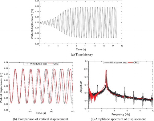
Table 3. Comparison with experimental results.

Calculation method	Maximum vertical displacement (m)	Dominant frequency (Hz)
Wind tunnel test	0.0294	2.813
Numerical simulation	0.0289	2.718
Difference ratio	1.7%	3.3%

3.2. Vortex-induced force

In the wind tunnel tests (Zhu et al., 2013), the fluctuating force obtained through the balance contains four parts: the pure vortex-induced force on the oscillating girder, the inertia force of the model, the non-wind-induced additional inertia force, and the non-wind-induced additional damping force. The non-wind-induced additional force (including both the inertia and damping components) can be represented as (9) where is the non-wind-induced additional force; are the velocity and the acceleration of the girder; m₀ and c₀ are the non-wind-induced additional mass and damping coefficient, respectively. m₀ and c₀ can be identified though free vibration of the girder with zero wind speed condition.

Comparatively, the fluctuating force in the simulation contains the pure vortex-induced force, the non-wind-induced additional inertia force, and the non-wind-induced additional damping force. Consequently, the vortex-induced force needs to be calculated through subtracting of the non-wind-induced additional inertia and damping force from the total force, as (10) where is the fluctuating part of the lift force; and is the vortex-induced force. With a free vibration in the zero wind speed condition, . As a result, m₀ and c₀ can be identified directly from Eq. (10). They are 6.051 kg and 3.098 N·s/m in this study, respectively.

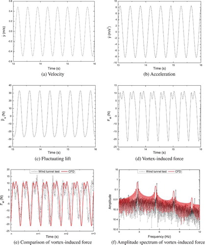
Figure 4(a–c) display the time histories of , , at the resonance stability period in the simulation. The vortex-induced forces of the girder are obtained through Eq. (10) and shown in Figure 4(d). The vortex-induced force and amplitude spectrum, calculated via CFD results, are compared with the experimental results (Zhu et al., 2013), as shown in Figure 4(e,f). It can be seen that the vortex-induced force from the simulation and the wind tunnel tests agree with each other. The one calculated from the wind tunnel test is not very smooth maybe due to the measurement error, while the one calculated by CFD is smooth and stable. The vortex-induced forces in both wind tunnel test and CFD present a fairly strong multiple-frequency characteristic, which can be interpreted as a symbol of nonlinear behavior of the vortex-induced force.

Figure 4. Vertical responses and vortex-induced force at resonance stability period.

4. Self-adaptive nonlinear fitting and vortex-induced force model

4.1. Self-adaptive nonlinear fitting method

A reasonable and reliable mathematical model for the vortex-induced force is the basic premise for the analysis of vortex-induced vibration. Vortex-induced force on a structure depends on the displacement y, time derivatives of the structure. In Scanlan’s empirical linear model (Simiu & Scanlan, 1996), linear terms of y and are involved. In Scanlan’s empirical nonlinear model (Simiu & Scanlan, 1996), a nonlinear term beside the linear terms of y and is adopted. Zhu et al. (2013) improved Scanlan’s empirical nonlinear model by adding another nonlinear term. Considering all the linear and nonlinear terms, a general form for the vortex-induced force can be expressed as (11) where is the air density; U is the wind speed; D is the height of the girder; is the circular frequency of vortex shedding; is the phase difference between the vortex shedding and displacement response; i and j are the order of and y, respectively; P_ij are the coefficients.

In order to determine the terms of the vortex-induced force model in Eq. (11) for the flat-steel-box girder appropriately, a Self-adaptive Nonlinear Fitting Method (SANFM) is proposed. In this process, nonlinear least square fitting based on Newton-Raphson method is utilized to get a fitted vortex-induced force model . The residue between and the vortex-induced force can be expressed as (12) where n is the number of data points. The object of the self-adaptive nonlinear fitting process is to get acceptable vortex-induced force model with small residue R. And is fitted to get at each time step.

At first, is obtained without the term in Eq. (11). A first residue R₀ is calculated using Eq. (12). Later on, progressively increasing i and j with increment of 1 in the expression of in Equation (11). New is obtained by nonlinear least square fitting, and the residue of the k^th pair of (i, j)_k is calculated as R_k. Also, a criterion is developed to judge whether the k^th pair of (i, j)_k is acceptable. In this study, the relative residue is taken as (13) In this study, the critical value of is 1%. If , (i, j)_k is accepted and the i^th order of and j^th order of y are selected in the vortex-induced force model. If , (i, j)_k is not accepted. Through the above process, the vortex-induced force model can be obtained in a self-adaptive way.

4.2. Effectiveness of SANFM

The typical vortex-induced vortex models for bridges, e.g. Scanlan (1981)and Larsen et al. (2000), were proposed mostly based on the responses of vortex-induced vibration, aiming at reflecting the response characteristics. Thus, they are closing processes without the participation of vortex-induced forces, which may result in inaccuracy prediction of the vortex-induced forces and the displacement responses. To fulfill the ends, an advanced nonlinear mathematical model was proposed by Zhu et al. (2013)as follows (14) whereY₁, Y₂, Y₃, ε and C_L are the coefficients of the model. Aimed to check the effectiveness, the mathematic model of the vortex-induced force tested by Zhu are determined through SANFM.

The process of SANFM is shown in Table 4. The final vortex-induced force model is (15)

Table 4. Process of SANFM for tested vortex-induced force.

k	Pij included in the model	Rk	(%)	Rk/max. FVI	Accepted
0	–	60.117	–	2.550	–
1	P10	41.669	30.686	1.767	Yes
2	P10, P01	31.546	24.295	1.338	Yes
3	P10, P01, P20	29.997	4.910	1.272	Yes
4	P10, P01, P20, P11	8.671	71.092	0.368	Yes
5	P10, P01, P20, P11, P02	7.777	10.313	0.330	Yes
6	P10, P01, P20, P11, P02, P30	7.069	9.110	0.300	Yes
7	P10, P01, P20, P11, P02, P30, P21	6.082	13.958	0.258	Yes
8	P10, P01, P20, P11, P02, P30, P21, P12	6.081	0.011	0.258	No
9	P10, P01, P20, P11, P02, P30, P21, P03	6.007	1.230	0.255	Yes
10	P10, P01, P20, P11, P02, P30, P21, P03, P40	6.007	0.003	0.255	No
11	P10, P01, P20, P11, P02, P30, P21, P03, P31	5.992	0.251	0.254	No
12	P10, P01, P20, P11, P02, P30, P21, P03, P22	5.995	0.196	0.254	No
13	P10, P01, P20, P11, P02, P30, P21, P03, P13	5.996	0.186	0.254	No
14	P10, P01, P20, P11, P02, P30, P21, P03, P04	5.984	0.385	0.254	No

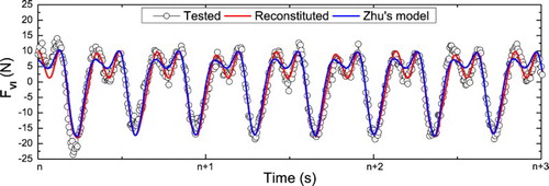
Through SANFM, more 2nd and 3th terms appear compared with the model in Eq. (14). Figure 5(a) shows the comparison between the vortex force predicted using Eq. (15) and Eq. (14) and the tested one. It can be seen that Zhu’s model cannot predict the vortex-induced force accurately at the position of peaks, and the model determined through SANFM is more precise to reconstitute the vortex-induced force.

Figure 5. Comparison of the vortex-induced force models.

4.3. Vortex-induced force model based on CFD

As in Section 4.2, the effectiveness of SANFM is validated based on the tested vortex-induced force. In this section, the vortex-induced force model based on the simulation is determined. The process of SANFM is shown in Table 5. The final mathematical model of vortex-induced force for the flat-steel-box girder is (16)

Table 5. Process of SANFM for calculated vortex-induced force.

k	Pij included in the model	Rk	(%)	Rk/max. FVI	Accepted
0	–	36.555	–	2.680	–
1	P10	33.245	9.055	2.437	YES
2	P10, P01	31.277	5.921	2.293	YES
3	P10, P01, P20	25.083	19.802	1.839	YES
4	P10, P01, P20, P11	20.930	16.558	1.534	YES
5	P10, P01, P20, P11, P02	2.600	87.577	0.191	YES
6	P10, P01, P20, P11, P02, P30	1.076	58.618	0.079	YES
7	P10, P01, P20, P11, P02, P30, P21	0.282	73.761	0.021	YES
8	P10, P01, P20, P11, P02, P30, P21, P12	24.283	−8500.945	1.780	NO
9	P10, P01, P20, P11, P02, P30, P21, P03	0.278	1.535	0.020	YES
10	P10, P01, P20, P11, P02, P30, P21, P03, P40	9.380	−3274.161	0.688	NO
11	P10, P01, P20, P11, P02, P30, P21, P03, P31	8.485	−2951.978	0.622	NO
12	P10, P01, P20, P11, P02, P30, P21, P03, P22	0.838	−201.499	0.061	NO
13	P10, P01, P20, P11, P02, P30, P21, P03, P13	0.100	64.089	0.007	YES

Compared with Eq. (15), is added. From Table 5, the vortex-induced force model using Eq. (15) has a very low relative residue (R_k/max. F_VI) of 0.02. The additional term decreases the residue nearly to zero. Table 6 shows the model parameters in Eq. (16). Figure 6(a) displays the comparison of the simulated and reconstituted vortex-induced vertical force of this model. It can be seen that the reconstituted vortex-induced force is in conformity with the simulated one. Figure 6(b,c) show the comparison between the simulated displacement through CFD and the solved displacement response using the vortex-induced force model. It can then be found that these two time histories agree well with each other. It can be concluded that the above results demonstrate the reliability and accuracy of the new mathematical model of vortex-induced force through SANFM for the flat-steel-box girder. In this model: the components and are the linear aerodynamic damping force and the linear aerodynamic stiffness force respectively; the pure high-order speed components represent the nonlinear aerodynamic damping forces; the pure high-order displacement components represent the nonlinear aerodynamic stiffness forces; and the cross terms provide both aerodynamic damping and aerodynamic stiffness.

Figure 6. Comparison of vortex-induced force and displacement.

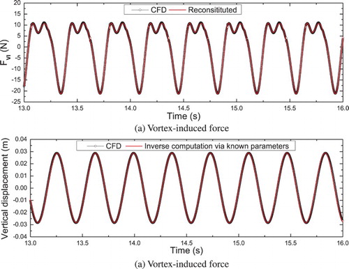
Table 6. Parameters of vortex-induced force model.

7.226	−0.381	−75.243	8.786	8.239	1011.060
347.124	−15.539	−313.002	0.195	17.325	1.156

5. Contribution analysis of components and location

5.1. Contribution factor

The components of the vortex-induced force are decomposed from each term in the expression of the model in Eq. (16). In order to analyze the effects of each component, a contribution factor is defined based on energy spectrum. Fourier transform is firstly used for the signal processing, as shown in Eq. (17).Thus, the amplitude spectrums of each component and the total vortex-induced force are obtained. Then the energy spectrums are obtained, which are the square of the amplitude spectrums. The contribution factor is defined as C_O, as shown in Eq. (18). (17) (18) where j is the number of each component and ranges from 1 to 10; is the j^th component of the vortex-induced force; and are the spectrum of the j^th component and the total vortex-induced force, respectively; and is the contribution factor of the j^th component at frequency.

5.2. Contribution of components

Through the contribution factor introduced above, the contributions of the ten components in Eq. (16) to three main frequencies (Base-frequency, Double-frequency, and Treble-frequency) are obtained, as shown in Table 7. It can be seen that the dominant frequency of the first-order terms (P₁₀, P₀₁) is 2.718 Hz, equal to the natural frequency of the girder. The dominant frequency of the second-order terms (P₂₀, P₁₁, P₀₂), the third-order terms (P₃₀, P₂₁, P₀₃), and the fourth-order term (P₁₃) is the double, the triple, and the four times of the natural frequency. The vortex-shedding force () corresponds to the natural frequency. It also can be found that the second-order terms (P₂₀, P₁₁, P₀₂) take a considerable proportion of 93.3% to the double-frequency of 5.422 Hz. The third-order terms (P₃₀, P₂₁, P₀₃) take a significant proportion of 99.6% to the triple-frequency and also take a remarkable proportion of 18.0% to the base-frequency of 2.713 Hz. It means that the high-order frequencies can be presented by high-order terms, and the responses of the vortex-induced force with high-order frequencies can be reconstituted via the model with high-order terms. Furthermore, the vortex-shedding force hardly contributes to high-order frequencies, but takes a proportion of 5.2% to the base-frequency. It can be concluded that the vortex-shedding frequency approximately equal to the base-frequency.

Table 7. Contribution factors of vortex-induced force components.

		Contribution factor (%)
Components	Dominant frequency (Hz)	Base-frequency	Double- frequency	Treble- frequency
P10	2.718	44.871	0.093	0.339
P01	2.718	31.914	0.002	0.003
P20	5.436	0.001	36.541	0.045
P11	5.436	0.001	19.397	0.004
P02	5.436	0.029	37.388	0.038
P30	8.154	11.847	0.001	43.050
P21	8.154	3.837	0.004	48.420
P03	8.154	2.290	0.009	8.092
P13	10.872	0.000	6.520	0.000
VS	2.718	5.211	0.043	0.009

Force-displacement phase plane is adopted (Figure 7) to analyze the energy evolution of each vortex-induced force component at one cycle of resonance stability period. The vertical displacement is defined as x-axis, the vortex-induced force is taken as y-axis.

Figure 7. Energy evolution of components.

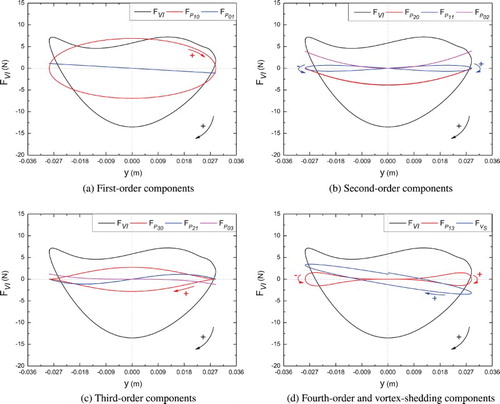
From Figure 7, the linear aerodynamic damping term forms an ellipse along the clockwise direction, so it inputs energy to VIV. The linear aerodynamic stiffness term forms a straight line across the second and the fourth quadrants, doing no work to VIV. The second-order aerodynamic damping term forms a vertical-axis symmetric parabolic at the third and the fourth quadrants, so it has nothing to do with the energy. The second-order cross term forms a biaxial symmetry figure-of-eight curve, and it inputs energy to VIV with positive displacement and dissipate energy when the displacement is negative, but the energy keeps balance within a cycle. The second-order aerodynamic stiffness term forms a vertical-axis symmetric parabolic at the first and the second quadrants, it also has nothing to do with the energy. The third-order aerodynamic damping term forms a closed curve like a nucleus of jujube, and it inputs energy to VIV. The other two third-order terms and are both centrosymmetric curves, doing no work. The fourth-order cross term forms a similar curve with the second-order cross term , so it has the same characteristics with . The vortex-shedding force forms a centrosymmetric ellipse across the second and the fourth quadrants with quite small values, so it inputs little energy to VIV. It can be found that, at the resonance period of VIV, the linear and the third-order aerodynamic damping forces input most of the energy to VIV.

5.3. Contribution of location

The girder without auxiliary takes 99.2% in terms of the contribution to vortex-induced force. Thus, this study focuses on the surface of the girder without auxiliary elements. In order to analyze the contribution of different location, the surface of the girder is divided into eight parts (see Figure 8). They are the underside of upstream web (UnUW), the upstream floor (UF), the downstream floor (DF), the underside of downstream web (UnDW), the upper of downstream web (UpDW), the downstream roof (DR), the upstream roof (UR) and the upper of upstream web (UpUW).

Figure 8. Partition of girder.

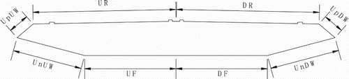
Table 8 shows the contribution factors of each part to the vortex-induced force components and the total vortex-induced force. Figure 9 shows the streamline and the Q-isolines (Hunt, Wray, & Moin, 1988) around the girder in a time period T. The roof (including both upstream and downstream roofs) makes up 79.03% of the total vortex-induced force, which can also be reflected in Figure 9. In Figure 9, a main vortex forms on the upstream roof, moves along the roof to the downstream roof, and sheds from the end of the downstream roof. The vortex development on the roof is the main source of the vortex-induced force of the flat-steel-box girder. The vortex-induced force on the underside of downstream web takes 9.17% of the total force, which is caused by another vortex developed under the downstream web (see Figure 9). As described in Section 5.2, the linear and the third-order aerodynamic damping forces and contribute to the total aerodynamic damping. Like the total vortex-induced force, the roof and the underside of downstream web take most of the aerodynamic damping. Meanwhile, the downstream web makes more than 5% contribution to the aerodynamic damping. The linear, third-order, and the fourth-order aerodynamic stiffness forces , , and contribute to the total aerodynamic stiffness. The roof takes most of the aerodynamic stiffness. For the linear aerodynamic stiffness term, upstream floor and underside of upstream web are the second most important positions. However, the underside of downstream web and downstream floor are the second most important positions for the high-order aerodynamic stiffness terms and .

Figure 9. Streamline around girder within one cycle.

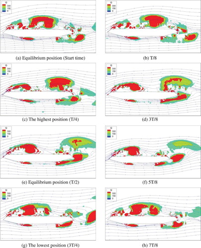
Table 8. Contribution of location to vortex-induced force (%).

Position	P10	P01	P20	P11	P02	P30	P21	P03	P13	VS	FVI
UnUW	4.17	8.75	0.19	1.10	1.88	0.50	1.48	0.28	2.11	0.23	1.49
UF	1.20	20.11	2.31	0.39	3.26	10.77	0.79	1.15	1.04	0.61	3.36
DF	7.76	5.12	0.01	1.98	5.53	3.18	5.26	6.55	4.40	2.27	4.26
UnDW	6.32	1.30	3.32	25.66	6.13	24.76	3.64	2.49	9.26	1.91	9.17
UpDW	3.27	1.01	1.86	1.26	0.11	5.20	1.21	1.94	2.17	2.70	1.55
DR	41.61	13.33	40.21	53.7	7.75	23.97	70.39	75.30	69.92	36.08	42.08
UR	34.58	49.87	50.58	15.57	74.86	31.06	16.92	12.28	10.88	55.6	36.95
UpUW	1.09	0.51	1.52	0.34	0.48	0.56	0.31	0.01	0.22	0.60	1.14

As the flow might separates at the surface corners of the girder, another surface division including corners is shown in Figure 10. The upper, middle, and underside upstream corners are arranged in Parts UpUC, UC, UnUc, respectively. The upper, middle, and underside downstream corners are set in Parts UpDC, DC, and UnDC, respectively. The middle parts of the roof and floor without any corner are chosen as Part MR and MF, respectively.Table 9 shows the contribution factors to the vortex-induced force and components with this surface division. The vortexes on the roof mainly are generated from the upper upstream corner and influenced by the upper downstream corner. In this regard, Parts UpUC, MR, and UpDC are counted together and take 80.45% of the vortex-induced force, which is consistent with the observation that the roof makes up the most vortex-induced force. From the flow development in Figure 9, the underside upstream corner, the underside downstream corner, and the middle downstream corner take responsibility for the flow separation. It can be seen in Table 9 that Part UnUC and Part MF (corresponding to the underside upstream corner) provides 27.04% of the linear aerodynamic stiffness term and 12.58% of the third-order aerodynamic damping term. Part UnDC (corresponding to the underside downstream corner) takes 13.64% of the third-order aerodynamic damping term and more than 5% of the linear aerodynamic damping term and the high-order aerodynamic stiffness term. Part DC (corresponding to the middle downstream corner) makes up the 15.08% of the third-order aerodynamic damping term and more than 5% of the high-order aerodynamic stiffness term.

Figure 10. Partition of girder including corners.

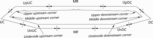
Table 9. Contribution of location including corners to vortex-induced force (%).

Position	P10	P01	P20	P11	P02	P30	P21	P03	P13	VS	FVI
UC	2.61	4.71	0.75	0.73	1.19	0.56	0.92	0.15	1.14	0.39	1.35
UnUC	2.67	14.36	1.22	0.78	2.56	5.56	1.08	0.67	1.54	0.42	2.42
MF	4.49	12.68	1.18	1.16	4.43	7.02	3.07	3.88	2.72	1.44	3.77
UnDC	7.01	3.15	1.63	13.51	5.81	13.64	4.4	4.52	6.73	2.09	6.53
DC	4.75	1.14	2.54	13.77	3.17	15.08	2.42	2.13	5.8	2.16	5.44
UpDC	24.86	7.95	23.41	30.46	4.32	16.16	39.79	42.88	40.04	21.49	24.17
MR	33.79	28.07	40.35	30.78	36.68	24.46	38.78	38.95	35.9	40.76	35.19
UpUC	19.82	27.94	28.92	8.81	41.84	17.52	9.54	6.82	6.13	31.25	21.09

6. Conclusions

Studies on the vortex-induced force of a flat-steel-box girder are carried out through CFD simulation with SST k-ω turbulence model in this study. A CFD numerical model is set up. Using the local remeshing method and elastic smoothing method, the movement of the girder is achieved. Through the independence studies, an effective time step and mesh scheme is determined. The simulation results are validated with the previous wind tunnel tests, it could be found that the numerical simulation method is reliable with high accuracy. The vortex-induced force on the flat-steel-box girder presents a fairly strong multiple-frequency characteristic.

A Self-adaptive Nonlinear Fitting Method (SANFM) is proposed based on Newton-Raphson method. The effectiveness of SANFM is validated on the tested vortex-induced force in the wind tunnel. Then the mathematical model of the vortex-induced force for the flat-steel box girder based on CFD is determined via SANFM. To account the effects of the components in the model and the effects of surface location to the vortex-induced force, a contribution factor is defined based on the energy spectrum. The linear and the third-order aerodynamic damping terms input most of the energy to the VIV. The roof of the flat-steel-box girder makes up 79.03% of the total vortex-induced force, and the vortex development on the roof is the main source of the vortex-induced force. The roof takes most of the aerodynamic damping terms including the first linear and the third-order terms. The flow separation from the underside upstream corner, the underside downstream corner and the middle downstream comer has large contribution to the third-order aerodynamic damping. Besides the roof, the flow separation from the underside upstream corner has great contribution to the linear aerodynamic stiffness term, while the flow separation near the underside downstream corner and the middle downstream corner has certain contribution to the high-order aerodynamic stiffness term.

Disclosure statement

No potential conflict of interest was reported by the authors.

Additional information

Funding

The authors are grateful for the financial supports from the Open Subject of State Key Laboratory of Disaster Reduction in Civil Engineering (SLDRCE14-01), the Sichuan Province Youth Science and Technology Innovation Team (2015TD0004), the National Natural Science Foundation of China (51478360, 51508480).

References

- Batina, J. T. (1990). Unsteady Euler airfoil solutions using unstructured dynamic meshes. AIAA Journal, 28(8), 1381–1388. doi: 10.2514/3.25229
- Bearman, P. W. (2011). Circular cylinder wakes and vortex-induced vibrations. Journal of Fluids and Structures, 27(5), 648–658. doi: 10.1016/j.jfluidstructs.2011.03.021
- Diana, G., Resta, F., Belloli, M., & Rocchi, D. (2006). On the vortex shedding forcing on suspension bridge deck. Journal of Wind Engineering and Industrial Aerodynamics, 94(5), 341–363. doi: 10.1016/j.jweia.2006.01.017
- Ehsan, F., & Scanlan, R. H. (1990). Vortex-induced vibrations of flexible bridges. Journal of Engineering Mechanic, 116(6), 1392–1411. doi: 10.1061/(ASCE)0733-9399(1990)116:6(1392)
- Fluent, F. (2006). FLUENT 6.3 user’s guide. Fluent Inc.
- Fujino, Y., & Yoshida, Y. (2002). Wind-induced vibration and control of trans-Tokyo Bay crossing bridge. Journal of Structural Engineering, 128(8), 1012–1025. doi: 10.1061/(ASCE)0733-9445(2002)128:8(1012)
- Guilmineau, E., & Queutey, P. (2002). A numerical simulation of vortex shedding from an oscillating circular cylinder. Journal of Fluids and Structures, 16(6), 773–794. doi: 10.1006/jfls.2002.0449
- Hallak, P. H., Pfeil, M. S., de Oliveira, S. R., Battista, R. C., de Sampaio, P. A., & Bezerra, C. M. (2013). Aerodynamic behavior analysis of Rio-Niterói bridge by means of computational fluid dynamics. Engineering Structures, 56, 935–944. doi: 10.1016/j.engstruct.2013.06.010
- Huang, L., Liao, H. L., Wang, B., & Li, Y. L. (2009). Numerical simulation for aerodynamic derivatives of bridge deck. Simulation Modelling Practice and Theory, 17(4), 719–729. doi: 10.1016/j.simpat.2008.12.004
- Hunt, J. C. R., Wray, A. A., & Moin, P. (1988). Eddies, streams, and convergence zones in turbulent flows. Report CTR-S88, Center For Turbulence Research. Retrieved from https://ntrs.nasa.gov/archive/nasa/casi.ntrs.nasa.gov/19890015167.pdf.
- Kumar, D. A., & Dalal, A. (2006). Numerical simulation of unconfined flow past a triangular cylinder. International Journal for Numerical Methods in Fluids, 52(7), 801–821. doi: 10.1002/fld.1210
- Laima, S. J., Li, H., Chen, W. L., & Li, F. C. (2013). Investigation and control of vortex-induced vibration of twin box girders. Journal of Fluids and Structures, 39, 205–221. doi: 10.1016/j.jfluidstructs.2012.10.009
- Larsen, A. (1995). A generalized model for assessment of vortex-induced vibrations of flexible structures. Journal of Wind Engineering and Industrial Aerodynamics, 57(2), 281–294. doi: 10.1016/0167-6105(95)00008-F
- Larsen, A., Esdahl, S., Andersen, J. E., & Vejrum, T. (2000). Storebaelt suspension bridge–vortex shedding excitation and mitigation by guide vanes. Journal of Wind Engineering and Industrial Aerodynamics, 88(2), 283–296. doi: 10.1016/S0167-6105(00)00054-4
- Li, H., Laima, S. J., Ou, J. P., Zhao, X. F., Zhou, W. S., Yu, Y., … Liu, Z. Q. (2011). Investigation of vortex-induced vibration of a suspension bridge with two separated steel box girders based on field measurements. Engineering Structures, 33(6), 1894–1907. doi: 10.1016/j.engstruct.2011.02.017
- Meng, X. L. (2013). Nonlinear behavior and mechanism of vertical vortex-induced vibration of long span steel-box-deck bridges. Shanghai, China: Tongji University.
- Sarkar, P. P., Caracoglia, L., Haan, F. L., Sato, H., & Murakoshi, J. (2009). Comparative and sensitivity study of flutter derivatives of selected bridge deck sections, part 1: Analysis of inter-laboratory experimental data. Engineering Structures, 31(1), 158–169. doi: 10.1016/j.engstruct.2008.07.020
- Sarwar, M. W., & Ishihara, T. (2010). Numerical study on suppression of vortex-induced vibrations of box girder bridge section by aerodynamic countermeasures. Journal of Wind Engineering and Industrial Aerodynamics, 98(12), 701–711. doi: 10.1016/j.jweia.2010.06.001
- Scanlan, R. H. (1981). State-of-the-art methods for calculating flutter, vortex-induced, and buffeting response of bridge structures (Report No. FHWA / RD-80 / 050). Washington, DC: Federal Highway Administration.
- Simiu, E., & Scanlan, R. H. (1996).Wind effects on structures (3rd ed.). New York, NY, USA: John Wiley and Sons Inc.
- Sumner, D. (2010). Two circular cylinders in cross-flow: A review. Journal of Fluids and Structures, 26(6), 849–899. doi: 10.1016/j.jfluidstructs.2010.07.001
- Sun, D., Owen, J. S., & Wright, N. G. (2009). Application of the k–ω turbulence model for a wind-induced vibration study of 2D bluff bodies. Journal of Wind Engineering and Industrial Aerodynamics, 97(2), 77–87. doi: 10.1016/j.jweia.2008.08.002
- Sun, Y. G., Li, M. S., & Liao, H. L. (2013). Investigation on vortex-induced vibration of a suspension bridge using section and full aeroelastic wind tunnel tests. Wind and Structures, 17(6), 565–587. doi: 10.12989/was.2013.17.6.565.
- Tamura, T. (1999). Reliability on CFD estimation for wind-structure interaction problems. Journal of Wind Engineering and Industrial Aerodynamics, 81(1), 117–143. doi: 10.1016/S0167-6105(99)00012-4
- Wang, B., Xu, Y. L., Zhu, L. D., Cao, S. Y., & Li, Y. L. (2013). Determination of aerodynamic forces on stationary/moving vehicle-bridge deck system under crosswinds using computational fluid dynamics. Engineering Applications of Computational Fluid Mechanics, 7(3), 355–368. doi: 10.1080/19942060.2013.11015477
- Williamson, C. H. K., & Govardhan, R. (2004). Vortex-induced vibrations. Annual Review of Fluid Mechanics, 36, 413–455. doi: 10.1146/annurev.fluid.36.050802.122128
- Wu, X. D., Ge, F., & Hong, Y. S. (2012). A review of recent studies on vortex-induced vibrations of long slender cylinders. Journal of Fluids and Structures, 28, 292–308. doi: 10.1016/j.jfluidstructs.2011.11.010
- Zhu, L. D., Meng, X. L., & Guo, Z. S. (2013). Nonlinear mathematical model of vortex-induced vertical force on a flat closed-box bridge deck. Journal of Wind Engineering and Industrial Aerodynamics, 122, 69–82. doi: 10.1016/j.jweia.2013.07.008