Assessment of the IDDES method acting as wall-modeled LES in the simulation of spatially developing supersonic flat plate boundary layers

ABSTRACT

The widely used improved delayed detached eddy simulation (IDDES) method is supposed to accurately predict the mean skin friction when it acts as wall-modeled large eddy simulation (WMLES), as claimed by the original authors. This property has been validated in subsonic flows but not in supersonic flows. In this article, IDDES acting as WMLES was assessed in the simulation of supersonic flat plate boundary layers, accompanied by two other hybrid Reynolds averaged Navier Stokes (RANS)/large eddy simulation (LES) methods which were also employed as WMLES, namely zonal detached eddy simulation (ZDES) and a hybrid RANS/LES method with the blending function proposed by Edwards and Choi (HRLMEC), for comparison. The underprediction of mean skin friction is existent in the results of IDDES but negligible in the results of ZDES and HRLMEC when all other settings are identical, presenting a contrast to the original idea of IDDES and some former research in subsonic flows. With the analysis of the shear stress, the underprediction of mean skin friction of IDDES is attributed to the underprediction of total Reynolds stress and turbulent kinetic energy production in the inner layer. Further research shows that, as for the present supersonic flow cases, IDDES can be capable of precisely predicting skin friction, but only if under the same condition the relevant LES, which uses the same subgrid-scale model, can precisely predict skin friction. This suggests that the problems met by IDDES may be essentially due to the intrinsic difficulty of LES to resolve the inner layer of a supersonic boundary layer: when resolving the inner layer of a supersonic boundary layer, LES should be tuned subtly and needs high computational cost, and may be damaged by any faulty factor, including but not limited to numerical resolution.

KEYWORDS:

• Hybrid Reynolds averaged Navier Stokes/large eddy simulation
• wall-modeled large eddy simulation
• improved delayed detached eddy simulation
• supersonic flat plate boundary layer
• skin friction

1. Introduction

Wall-bounded turbulent flows not only remain important in relatively simple configurations for academic turbulence research, but also play a vital role in many practical engineering applications. One of the basic features of wall-bounded turbulent flows is the multi-scale nature throughout the boundary layer, which becomes gradually distinct with increasing Reynolds number (Deck, Renard, Laraufie, & Sagaut, 2014; Larsson, Kawai, Bodart, & Bermejo-Moreno, 2016). Consequently, with increasing Reynolds number, severer constraints on the grid resolution are imposed on numerical simulation if using wall-resolved large eddy simulation (WRLES), in which all of the large energy-carrying scales throughout the boundary layer need to be resolved. Thus, WRLES is limited to the simulation of flows of low Reynolds number.

Another feature of wall-bounded turbulent flows is that the boundary layer can be divided into two parts: an inner layer which consists of small-scale structures such as quasi-streamwise vortices, and an outer layer which consists of large-scale structures. Fully resolving the small-scale structures in the inner layer requires the number of grid points following (Choi & Moin, 2012) or (Deck, Renard, Laraufie, & Sagaut, 2014). (Here is the Reynolds number based on the flat-plate length in the streamwise direction; is the Reynolds number based on the momentum thickness at ; is the free-stream velocity and is the free-stream kinematic viscosity.) In contrast, the number of grid points required for the outer layer is much smaller, following (Deck, Renard, Laraufie, & Sagaut, 2014) or not directly dependent on Reynolds number (Larsson et al., 2016). Hence it is preferable to resolve the large-scale structures of the outer layer, and model the structures in the inner layer, to dramatically reduce the cost while keeping the capacity of resolving the dominant large-scale structures. This is the principle of wall-modeled large eddy simulation (WMLES). There are various WMLES approaches and readers can refer to Larsson et al. (2016) for details. A widely used type of WMLES approach is hybrid Reynolds averaged Navier Stokes (RANS)/large eddy simulation (LES) methods using RANS in the inner layer as a wall model. In this article, all of the methods involved are of this type.

Numerous versions of hybrid RANS/LES methods have been proposed over the years (Menter, Schütze, & Gritskevich, 2012). It is worth mentioning that, although a few versions of hybrid RANS/LES methods can be used as WMLES, some other versions of hybrid RANS/LES simulations, for example delayed detached eddy simulation (DDES), are designed to resolve turbulence using LES only in the field of large or detached separation and to model turbulence using RANS in almost the whole boundary. The latter are beyond the scope of this article, because they are not proposed to provide a resolved turbulent boundary layer. As regards the former, there are still various versions, considering that different turbulent models of RANS, different subgrid-scale models of LES and different blending methods can be selected from; Larsson et al. (2016) can be referred to for details. In this article, three versions of hybrid RANS/LES methods are involved, namely improved delayed detached eddy simulation (IDDES) proposed by Shur, Spalart, Strelets, and Travin (2008), zonal detached eddy simulation (ZDES) proposed by Deck (2005) and a hybrid RANS/LES method (denoted as HRLMEC hereinafter) with the blending function proposed by Edwards, Choi, and Boles (2008). The most significant difference between these versions is the blending method, corresponding to how to prescribe the location of the RANS-to-LES interface and the transition across the interface. We focus on IDDES and use the other two versions for a comparison.

The philosophy of IDDES is combining DDES and WMLES, ensuring a different response depending on whether the grid resolution is sufficient to resolve dominant eddies in the boundary layer and whether the simulation contains inflow turbulence content. IDDES performs as WMLES if the grid resolution is sufficient and the simulation contains inflow turbulence, otherwise it reduces to DDES. IDDES has become popular in computational fluid dynamics (CFD) communities since it was proposed (e.g., see Krappel, Kuhlmann, Kirschner, Ruprecht, & Riedelbauch, 2015; Zhao, Zhang, & Xu, 2017), thanks to its three advantages. The first is that it can give generally good results while requiring no external user inputs, and in this respect it is superior to methods which need to predetermine the RANS-to-LES interface, such as ZDES and methods which require a precalibration, such as HRLMEC. The second advantage is that it is self-adaptive so that it can safely reduce to DDES when the demands of WMLES are not satisfied, and thus is robust for complex configurations. The third advantage is, as Shur et al. (2008) argue, that when acting as WMLES, IDDES eliminates the problems of log-layer mismatch and underprediction of skin friction, which WMLES methods commonly suffer from (Nikitin, Nicoud, Wasistho, Squires, & Spalart, 2000). These problems are to be further discussed in Section 2.

In subsonic wall-bounded turbulent flows, the good performance of IDDES acting as WMLES has been validated (e.g., see Shur, Spalart, Strelets, & Travin, 2014). However, Gieseking, Choi, Edwards, and Hassan (2011) showed that when used as WMLES in supersonic flat plates, IDDES could lead to a severe underprediction of skin friction up to 25% (see Figure 11 in Gieseking et al., 2011), which was distinctly inconsistent with the aim of IDDES. Yet in that paper, the results of IDDES were simply used for a comparison with the newly developed hybrid RANS/LES methods and the problem of IDDES was not further analyzed. Besides, Peterson and Candler (2011) showed that IDDES exhibited log-layer mismatch when it was used as WMLES in a supersonic flat plate. Although skin friction was not presented in their paper, it can be deduced that the underprediction certainly existed because it is always concomitant with log-layer mismatch. Yet they simply ascribed the log-layer mismatch to the fact that IDDES is calibrated using low-speed flow and no further analysis was undertaken because it was beyond the scope of their current investigation.

To the knowledge of the authors, when coming to the simulation of supersonic flows, in the published literature apart from Gieseking et al. (2011) and Peterson and Candler (2011) IDDES always simply acts as a DDES approach (e.g., see Wang, Piao, & Niu, 2015), and even in the limited literature published where IDDES acts as WMLES the issue of underprediction of skin friction is rarely discussed (e.g., see Cocks, Bruno, Donohue, & Haas, 2013). No detailed assessment of IDDES acting as WMLES has ever been conducted regarding the prediction of mean skin friction in supersonic boundary layer flows. Thus, it is valuable to develop an assessment of IDDES acting as WMLES in the simulation of supersonic wall-bounded turbulent flows. Among various configurations, a spatially developing zero pressure gradient (ZPG) supersonic flat plate boundary layer is representative. Despite its simplicity, this is the basis of many more complex flows of practical interest, especially those whose dynamics are strongly affected by the Lagrangian history of the upstream boundary layer. Thus, its simulation is a mandatory milestone in the assessment of any WMLES method intended for utility in complex flows. In this article, spatially developing ZPG supersonic flat plate boundary layers at two Reynolds numbers ( and ) are simulated by IDDES, and analyzed through a comparison with the results of ZDES and HRLMEC.

The rest of the article is organized as follows. In Section 2, the significant problem of underprediction of skin friction in hybrid RANS/LES methods is reviewed and discussed. Then in Section 3, numerical methods including time marching and spatial discretization schemes and inflow turbulent boundary conditions involved in this article are presented, as well as the hybrid RANS/LES methods. In Section 4, numerical settings are given, and then results of simulations are presented and discussed in detail. Finally, some concluding remarks are presented in Section 5.

2. Underprediction of skin friction in hybrid RANS/LES methods

Despite deficiency in many flows compared with LES (Georgiadis, Rizzetta, & Fureby, 2010), RANS methods with widely used turbulent models such as the Spalart-Allmaras model and Menter’s shear stress transport (SST) model show satisfying accuracy in a spatially developing ZPG flat plate boundary layer regarding mean flow quantities since they have been validated for the canonical boundary layer flows (Menter, 1994; Wilcox, 2006), and can be used as a reference for the velocity profile and skin friction prediction.

Underprediction of skin friction, which is concomitant with log-layer mismatch in hybrid RANS/LES methods acting as WMLES, has caught wide attention since Nikitin et al. (2000) detected it when applying a DES method as WMLES. Typically, the ultimate cause of underprediction of skin friction is the insufficient generation of energy-carrying eddies and resultant Reynolds stress near the interface where the RANS mode transits to the LES mode. Considering the streamwise momentum equation of Navier Stokes equations of an equilibrium boundary layer, it can be deduced that the resolved Reynolds stress term, modeled Reynolds stress term and viscous term together reach a balance. Here is the eddy viscosity corresponding to LES subgrid-scale model , or RANS model , or even a hybrid of and blended by a mathematic function. In the vicinity of the interface, is significantly lower than . Thus if resolved Reynolds stress is insufficient near the RANS/LES interface, velocity gradient reaches higher in order to obtain a balance. It further results in a reduction in the velocity close to the wall, leading to the underprediction of skin friction.

Remedies have been developed for this problem. One type is adding source terms that create velocity fluctuations to Navier Stokes equations to accelerate the development of resolved eddies near the RANS-to-LES interface (Piomelli, 2008). Another type is introducing empirical functions to lead a steep drop of the eddy viscosity to destabilize the flow in the LES region near the interface while elevating the eddy viscosity to prevent the excessive reduction of resultant modeled Reynolds stress in the RANS region near the interface, proposed by IDDES. Besides, better prediction of skin friction was reached by some researchers simply adjusting the location of the RANS-to-LES interface (Choi, Edwards, & Baurle, 2009; Deck, Weiss, Pamiés, & Garnier, 2011). For simulations of spatially developing boundary layers, all of the methods need to impose time-dependent turbulent content at the inflow as realistic as possible.

Although it is known that underprediction of skin friction is ultimately caused by the insufficient resolution of resolved eddies near the RANS-to-LES interface, the value of error of a specific case is closely related to many factors. Apart from difference between different versions of hybrid RANS/LES methods, the factors include, but are not limited to, inflow turbulence generation methods, numerical resolution which consists of time marching schemes and time step, spatial discretization schemes and grid resolution, and so forth. It may be confusing that although a certain hybrid RANS/LES method is claimed in published papers to be capable of precisely predicting skin friction, underprediction of skin friction still emerges at times when users utilize it themselves.

3. Numerical methods

The simulations in this article were conducted using the in-house CFD code AHL3D. This AHL3D code uses a three-dimensional, parallel, finite volume flow solver solving the compressible Navier Stokes equations on multi-block, structured meshes and has been validated by a vast array of applications (e.g., see Le, Yang, Liu, & Xing, 2005). The major methods involved in this article are introduced as follows.

3.1. Three versions of hybrid RANS/LES methods

Hybrid RANS/LES methods involved in this article share a background RANS turbulent model, namely Menter’s SST model (Menter, 1994). Modifications to the original SST model are realized by substituting the turbulent length scale of the destruction term in the k-transport equation. In the original SST model, . If is replaced by a length scale , the modified SST model can be used as a subgrid-scale model (Strelets, 2001). In this article, the three versions of hybrid RANS/LES methods involved use the same grid length scale set to proposed by Shur et al. (2008). A hybrid RANS/LES method can be fabricated by hybridizing the two different length scales using a blending function: (1) The blending function can either smoothly transit through a region from the inner layer to outer layer, or simply change abruptly at an interface.

3.1.1. IDDES

When used as a WMLES method, IDDES uses the length scale: (2) The manifestation of Equation (2) is slightly different from that of Equation (1) in that an elevating function is introduced to prevent the excessive reduction of the eddy viscosity in the RANS region near the interface. is defined as: (3) with , where is the distance to wall and is the maximum of grid length scale in three dimensions. The elevating function in Equation (2) is defined as: (4) Here: (5) (6) (7) (8) where and are empirical constants and set to 1.87 and 5.0 if the background RANS model is SST. is an empirical function and set to 1. More details can be acquired from Shur et al. (2008).

It can be concluded from that the RANS-to-LES transition takes place at about 0.6 to away from the wall. Later in Section 4 we can see that the interface of IDDES acting as WMLES locates either in the buffer layer or near the inner edge of the log layer, based on the setting of .

3.1.2. ZDES

Within ZDES, users need to set individual RANS and LES domains. There are three modes of ZDES, and mode III in which an interface position is prescribed is recommended if ZDES is supposed to be used as WMLES (Deck, 2012): (9) As far as we know, there are no strict criteria for the prescription of the RANS/LES transition location of ZDES. Nevertheless there is a general principle, as suggested by Deck, Renard, Laraufie, and Sagaut (2014, p. 1): ‘for a better skin friction prediction, it is shown that the RANS/LES interface should be high enough in the boundary layer’. In order to resolve the large-scale structures of the outer layer and model the structures in the inner layer, the interface can be located around the upper edge of the inner layer.

3.1.3. HRLMEC

The blending function proposed by (Edwards et al., 2008) is defined as: (10) Here is the von Kármán constant. is , in which = is a modeled form of the Taylor microscale. is a constant set to so that occurs at the location . is a constant chosen to enforce the average RANS-to-LES interface located at a prescribed position. This prescribed position is located at the position where the wake law starts to deviate from the log law: (11)

Here the superscript ‘+’ denotes the inner scaling: , and the subscript ‘vd’ denotes the van Direst transformation. More details can be found in Edwards et al. (2008).

3.2. Inflow turbulence generation

Among multifarious inflow turbulence generation methods, recycling/rescaling methods have been verified to be efficient to lead to a physically realistic field after a relatively short transition region for flat-plate-like flows. The series of recycling/rescaling methods originates from Lund, Wu, and Squires (1998), and Lund’s method was extended by Urbin, Knight, and Zheltovodov (2001) for compressible flows. Then various modifications to Urbin and Knight’s method were proposed. Here we utilize Edward’s method (Edwards et al., 2008). The principle is to extract the fluctuations at a station downstream from the inflow and then superimpose them onto a RANS mean-inflow profile after rescaling it to account for boundary layer growth: (12) where denotes the corresponding y_recycle of y_inlet in the recycling station, and denotes the rescaling factor. More details can be found in Edwards et al. (2008).

3.3. Time marching and spatial discretization

In this article, time marching is carried out by means of the second-order-accurate dual time-stepping scheme (Pulliam, 1993), with lower upper symmetric Gauss Seidel scheme (Jameson & Yoon, 1986) for an implicit approach. Three spatial discretization schemes are involved, namely an optimized low-dissipation scheme with a monotonicity preserving procedure (MPLD) developed by Fang, Li, and Lu (2013), an adaptive monotonic upstream-centered scheme for conservation laws (MUSCL) scheme proposed by Billet and Louedin (2001) and a blend of these two schemes based on a smoothness indicator, which is named the hybrid optimized low-dissipation and adaptive MUSCL scheme (denoted LAM for short hereinafter). Details of the blending method for the LAM scheme are given in Appendix 1. MPLD is a high-resolution, low-dissipation scheme, and is devised for refined simulations. Adaptive MUSCL has relatively higher dissipation which varies from that of conventional MUSCL to that of the widely used weighted essentially non-oscillatory schemes, and thus is suitable for simulations in large gradient or strong discontinuous regions. Because both types of simulations are widely existent in supersonic flows, the LAM scheme is chosen as the focal scheme. In this article, the influence of the dissipation of spatial discretization schemes is investigated through a comparison of their results.

4. Simulation settings, results and discussions

Because the uppermost motive of this article is to assess the IDDES method acting as WMLES on a supersonic flat plate boundary layer, cases of high Reynolds number are preferable. Thus first we tested a series of cases at a Reynolds number equal to 20,913 based on the momentum thickness at the inflow boundary . In these cases, the computational domain was set to L_x = , L_y = , L_z = . The boundary conditions included two periodic conditions in the spanwise direction, adiabatic wall and inflow conditions using a recycling/rescaling method whose recycling station was located at x = . The base grid was set to , and gradually stretching from 0.55 on the wall to 69 at the upper edge of the boundary layer using a hyperbolic tangent stretching function. The grid was not well refined, but nevertheless practical in hybrid RANS/LES simulations. The time step was set to 2.0E^–7 s. The other flow parameters are presented in Table 1 and the numerical settings are presented in Table 2. Case 1.1 was selected as the base case. In Case 1.2 the HRLMEC blending function was utilized instead of IDDES. In Case 1.3 the low dissipation scheme MPLD was utilized instead of LAM. In Case 1.4 a densified grid set to , and gradually stretching from 0.39 on the wall to 48 at the upper edge was utilized to test the effect of grid resolution.

Table 1. Flow parameters.

Flow						Inflow momentum thickness (mm)	Inflow boundary layer thickness (mm)
F1	20913	3615	2.0	25,266	151.2	0.754	9.0
F2	2105	228	2.9	2296	108.1	0.353	5.18

Table 2. Numerical settings of Flow 1.

Case	Flow	Blending	Spatial discretization					Nx	Nz	Nyb
1.1	F1	IDDES	LAM	165	69	0.55	69	350	173	144
1.2	F1	HRLMEC	LAM	165	69	0.55	69	350	173	144
1.3	F1	IDDES	MPLD	165	69	0.55	69	350	173	144
1.4	F1	IDDES	LAM	116	48	0.39	48	498	249	180

The size of the computational domain is L_x = , L_y = , L_z = . is at the wall and is at the edge of the boundary layer. N_x and N_z are the numbers of grid points in x and z directions, and N_yb is the number of grid points in y direction in the boundary layer.

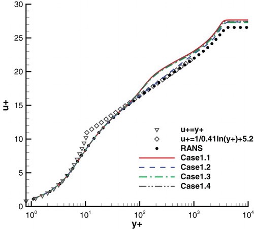
As noted in Section 2, regarding mean flow quantities the RANS results of a spatially developing ZPG flat plate boundary layer are satisfactory and thus adequate as benchmark solutions. Figure 1 shows the streamwise distribution of the friction coefficient Cf. In this figure and the figures which illustrate the streamwise distribution of Cf hereinafter, the meaningful comparison between different approaches is performed from the recycling station onward, since the upstream region is used as the adaptation region for the inlet fluctuations to generate real turbulence. The gray shadow presents an area in which Cf deviates from the RANS result under 6%. When the LAM scheme is used, the error of IDDES is slightly larger than that of HRLMEC, despite both methods providing acceptable results downstream from the inflow section. When we improve the resolution of the numerical schemes in Case 1.3, the error of IDDES is reduced, indicating that numerical resolutions have certain influence on the results of IDDES. A similar trend occurs when the grid is densified in Case 1.4. Figure 2 shows the velocity profiles at x = 11. From this we can see that, regarding the velocity profile, the result of IDDES significantly deviates from the log law starting from about y⁺ = 100, while the result of HRLMEC obeys the log law well.

Figure 1. Comparison of the distributions of the mean friction coefficient Cf of Cases 1.1–1.4.

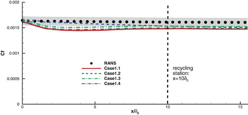
Figure 2. Comparison of the velocity profiles at x = 11δ₀ of Cases 1.1–1.4.

Aiming at a more detailed and clearer analysis with much fewer computational resources, a series of cases at a much lower Reynolds number, namely at which the IDDES method is sufficient to act as WRLES, were simulated. In these cases, the base computational domain was set to L_x = , L_y = , L_z =  and an additional computational domain which doubled the spanwise extension was used to check the effect of domain size. The boundary conditions included two periodic conditions in the spanwise direction, an isothermal wall with wall temperature equal to 307 K and an inflow condition using a recycling/rescaling method whose recycling station was located at x = . The base grid was set to , and gradually stretching from 0.22 on the wall to 8.7 at the upper edge of the boundary layer using a hyperbolic tangent stretching function. Considering that the usual grid demands for WRLES of flat-plate-like configurations are and (Georgiadis et al., 2010), the base grid was fine enough even for a WRLES and could eliminate the effect of grid resolution that might be a possible factor on the accuracy in the high Reynolds number cases. Nevertheless, a densified grid set to , and gradually stretching from 0.165 to 6.4 was used to test of the effect of grid resolution for checking. The time step was set to 2.0E^–7 s leading to to meet the demand of proposed by Choi and Moin (1994). The other numerical settings are presented in Table 3. Case 2.1 was selected as the base case. In Case 2.2 an HRLMEC blending function was utilized instead of IDDES. In Case 2.3 a specific ZDES which fixed the RANS-to-LES interface at y⁺ = 37.5 was utilized instead of IDDES. For a further analysis of IDDES, in Case 2.4 a doubled domain size in the spanwise direction was utilized and in Case 2.5 a densified grid was utilized compared with the base case. In order to make a further analysis of the numerical schemes, the relatively low dissipation scheme MPLD and relatively high dissipation scheme adaptive MUSCL were utilized for IDDES in Case 2.6 and Case 2.7, for HRLMEC in Case 2.8 and Case 2.9, and for ZDES in Case 2.10 and Case 2.11.

Table 3. Numerical settings of Flow 2.

Case	Flow	Blending	Spatial discretization	Computational domain					Nx	Nz	Nyb
2.1	F2	IDDES	LAM	Base domain	14	8.7	0.22	8.7	261	74	110
2.2	F2	HRLMEC	LAM	Base domain	14	8.7	0.22	8.7	261	74	110
2.3	F2	ZDES	LAM	Base domain	14	8.7	0.22	8.7	261	74	110
2.4	F2	IDDES	LAM	Doubled domain size in the spanwise direction	14	8.7	0.22	8.7	261	148	110
2.5	F2	IDDES	LAM	Base domain	9.8	6.4	0.165	6.4	373	101	144
2.6	F2	IDDES	MPLD	Base domain	14	8.7	0.22	8.7	261	74	110
2.7	F2	IDDES	Adaptive MUSCL	Base domain	14	8.7	0.22	8.7	261	74	110
2.8	F2	HRLMEC	MPLD	Base domain	14	8.7	0.22	8.7	261	74	110
2.9	F2	HRLMEC	Adaptive MUSCL	Base domain	14	8.7	0.22	8.7	261	74	110
2.10	F2	ZDES	MPLD	Base domain	14	8.7	0.22	8.7	261	74	110
2.11	F2	ZDES	Adaptive MUSCL	Base domain	14	8.7	0.22	8.7	261	74	110
2.12	F2	WRLES	LAM	Base domain	14	8.7	0.22	8.7	261	74	110
2.13	F2	WRLES	MPLD	Base domain	9.8	6.4	0.165	6.4	373	101	144
2.14	F2	IDDES	MPLD	Base domain	9.8	6.4	0.165	6.4	373	101	144
2.15	F2	ZDES(*)	LAM	Base domain	14	8.7	0.22	8.7	261	74	110

The size of the base computational domain is L_x = , L_y = , L_z = . is at the wall and is at the edge of the boundary layer. N_x, and N_z are the numbers of grid points in x and z directions, and N_yb is the number of grid points in y direction in the boundary layer. The indicator (*) means that in Case 2.15 the RANS-to-LES interface of ZDES is changed to , compared with Case 2.3.

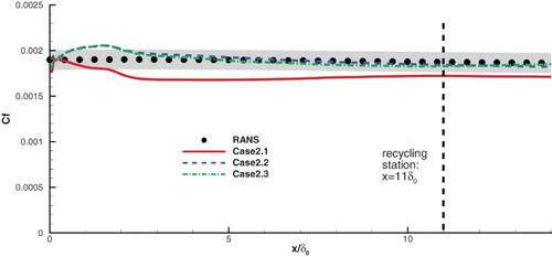
Figure 3 shows the streamwise distribution of the friction coefficient Cf of Cases 2.1–2.3. It can be seen that at a downstream position such as x = 12, under the same numerical scheme, namely LAM, the error of IDDES is 8.1%, which is markedly larger than that of ZDES and HRLMEC both of which are less than 2.0%. Note that IDDES was designed to eliminate the underprediction of Cf, and the correctness has been validated by a few simulations (e.g., see Shur et al., 2014) on channel flows and spatially developing flat plate boundary layers. However, as mentioned in Section 1, the validations were limited to subsonic flows and there are few publications treating IDDES acting as WMLES for supersonic flat plate boundary layers. Our results tally with Gieseking et al. (2011) in which the error of IDDES on Cf could be severely up to 25%, and are inconsistent with the aim of IDDES.

Figure 3. Comparison of the distributions of the mean friction coefficient Cf of Cases 2.1–2.3.

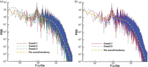
As mentioned in Section 1, the inflow turbulence generation method plays a vital role when IDDES acts as WMLES. Note that the inflow turbulence generation method used in this article has been validated to perform well in supersonic flows (Edwards et al., 2008). Nevertheless, here we give some extra evidence to ensure that the error of Case 2.1 is not due to the inflow turbulence generation. An instantaneous temperature image of Case 2.1 is illustrated in Figure 4. From this figure we can see that the large-scale unsteadiness in the outer zone of the developing boundary layer has indeed been generated. Next, the power spectral density (PSD) functions of the streamwise velocity component at y =  are illustrated in Figure 5 for Case 2.1, Case 2.2, Case 2.3 and Case 2.5 at x = , which is downstream of the recycling station. From Figure 5(a) we can see that the PSD function of Case 2.1 presents a similar overall tendency along the frequency axis to that of Case 2.2 and Case 2.3, which predict quite accurate Cf. From Figure 5(b) we can see that refining the grid of Case 2.1 does not significantly change the overall tendency of the PSD function, suggesting that the grid used in Case 2.1 is sufficient for generating and sustaining turbulence downstream of the recycling station. Besides, all of these profiles present a similar overall tendency to the profiles shown in Figure 4 of Deck et al. (2011). It is worth mentioning that these PSD functions exhibit a peak at about F.Lr/Ue = 0.9, indicating a nonphysical energy-carrying low-frequency component introduced by the recycling/rescaling method. Although this flaw can be harmful if studies are of interest on the unsteadiness of some downstream phenomena such as the shock/boundary layer interaction system, the influences on the prediction of the mean flow quantities such as velocity profile and Cf are negligible (e.g., see Morgan, Larsson, Kawai, & Lele, 2011).

Figure 4. An instantaneous temperature image of Case 2.1.

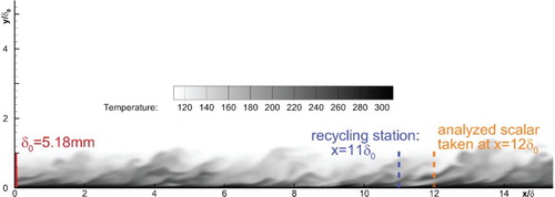
Figure 5. (a) Power spectral density (PSD) function of the streamwise velocity of Cases 2.1–2.3 at x = 12δ₀, y = 0.58δ₀. (b) PSD function of the streamwise velocity of Case 2.1 and Case 2.5 at x = 12δ₀, y = 0.58δ₀. F is the frequency; Lr is the distance between the recycling station and the inlet plane; Ue is the mean streamwise velocity at the edge of the boundary layer.

The performance of IDDES can be further analyzed using Cases 2.4–2.7 as shown in Figure 6. Comparing Case 2.4 with Case 2.1, it can be affirmed that the spanwise domain size of the base case is sufficient. Comparing Case 2.5 with Case 2.1, it can be seen that notwithstanding the grid resolution of the base case being sufficient for WRLES, improving the grid resolution does decrease the error of the Cf and leads to results similar to Case 2.6 which uses the low dissipation spatial scheme. Comparing Cases 2.6 and 2.7 with Case 2.1, it can be clearly inferred that the numerical scheme plays a significant role on Cf of IDDES, with more dissipation leading to larger error. However, as shown in Figure 7 and Figure 8, the numerical scheme has much less impact on the other two hybrid methods. These phenomena are to be explained later.

Figure 6. Comparison of the distributions of the mean friction coefficient Cf of Case 2.1 and Cases 2.4–2.7.

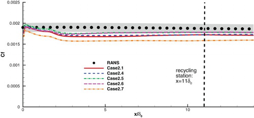
Figure 7. Comparison of the distributions of the mean friction coefficient Cf of Case 2.2 and Cases 2.8 and 2.9.

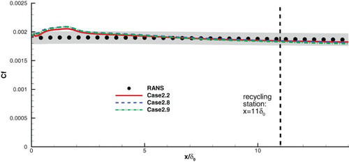
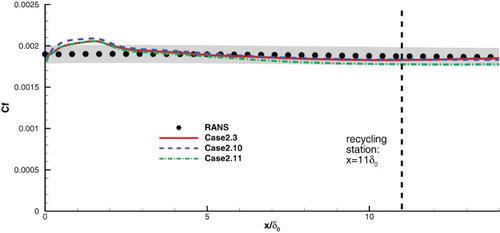
Figure 8. Comparison of the distributions of the mean friction coefficient Cf of Case 2.3 and Cases 2.10 and 2.11.

Because when we use the LAM scheme and the base grid resolution both ZDES and HRLMEC reach quite satisfying Cf, it is instructive to figure out why under the same conditions IDDES differs from the other two, and, further, in which mechanism the calculated friction coefficient is affected. Considering that the shear stress plays a key role in underprediction of Cf as mentioned in Section 2, we present in Figure 9 the total shear stress at a downstream position x = 12 of Cases 2.1–2.3 combined with that of RANS as a reference. Figure 9 also contains the distribution of the blending function . The distribution of the blending function reveals that the RANS-to-LES interface of IDDES lies either in the buffer layer or near the bottom of the log layer, radically different from that of ZDES and HRLMEC. While the total shear stress of ZDES and HRLMEC near the wall is close to that of RANS and consistent with the conclusion that the total shear stress is nearly constant in the inner layer of a turbulent boundary layer (Deck, Renard, Laraufie, & Weiss, 2014), the total shear stress of IDDES is severely depressed especially near the transition region. 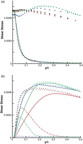Next, the total shear stress is decomposed into viscous stress and Reynolds stress: , and the latter can be further decomposed into the resolved part and the modeled part: . Each of these terms is presented in Figure 10. Clearly, in the inner layer IDDES produces larger resolved Reynolds stress, but not large enough to compensate for the lack of modeled Reynolds stress at . Besides, from Figure 10 we can see that the viscous stress of IDDES at about 0.03–0.08 which is around the IDDES transition region is larger than RANS, indicating that is incorrectly higher in this area and thus results in depressed velocity u down to the wall. This is consistent with the analysis in Section 2. From Figure 10 we can also see that in the outer layer ZDES overpredicts the resolved Reynolds stress even more than IDDES does. The reason for this is not clear, but a similar phenomenon is shown by Figure 17(a) in Deck et al. (2011). The overpredicted resolved Reynolds stress further leads to the overpredicted shear stress.

Figure 9. Blending function and total shear stress at x = 12δ₀ (RANS, black; Case 2.1, blue; Case 2.2, red; Case 2.3, green): •, total shear stress (nondimensionalized by ρ_∞); ━, fblend.

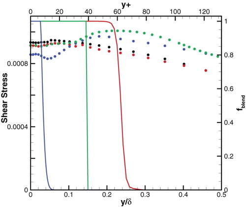
Figure 10. Decomposition of total shear stress (nondimensionalized by ρ_∞) at x = 12δ₀ (black, RANS; blue, Case 2.1; red, Case 2.2; green, Case 2.3): (a) circle, total shear stress; dashed line, viscous stress. (b) right triangle, total Reynolds stress; dashed dot line, modeled Reynolds stress; solid line, resolved Reynolds stress.

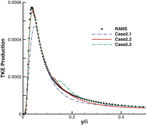
The effect of shear stress can be analyzed in an alternative way using the theory of Renard and Deck (2016), which suggests that the turbulent kinetic energy (TKE) production in the buffer layer dominates the mean skin friction of low Reynolds number flow. Figure 11 illustrates the TKE production of Cases 2.1–2.3. It can be seen that the TKE production of IDDES in the buffer layer is notably smaller than that of RANS, leading to smaller Cf, while the performances of both ZDES and HRLMEC approximate that of RANS.

Figure 11. TKE production at x = 12δ₀ of Cases 2.1–2.3 (nondimensionalized by /L_∞).

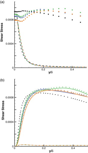
Decomposition of total shear stress for Case 2.1, Case 2.6, and Case 2.7 is presented in Figure 12. From this figure we can see that, in terms of IDDES, the numerical resolution has negligible effect on the modeled Reynolds stress, but significantly affects the resolved Reynolds stress and therefore affects the total shear stress in the inner layer. This accords with our intuition, because the transition region of IDDES is much nearer to the wall and thus the resolved Reynolds stress plays a more important role, compared with ZDES and HRLMEC. This can also explain why the numerical scheme has much less impact on Cf for ZDES and HRLMEC, as shown in Figure 7 and Figure 8.

Figure 12. Decomposition of total shear stress (nondimensionalized by ρ_∞) at x = 12δ₀ (black, RANS; blue, Case 2.1; green, Case 2.6; orange, Case 2.7): (a) circle, total shear stress; dashed line, viscous stress. (b) right triangle, total Reynolds stress; dashed dot line, modeled Reynolds stress; solid line, resolved Reynolds stress.

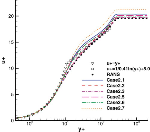
Although the error of shear stress in the inner layer for IDDES can be reduced by increasing the numerical resolution, it cannot be thoroughly eliminated in the inner layer, especially near the RANS-to-LES interface, as illustrated by Figure 12. A similar characteristic can be found in the velocity profiles. In Figure 13, the velocity profiles at x = 12are compared. We can see that when we use LAM scheme, IDDES shows deviation from RANS results and the log law while ZDES and HRLMEC exhibit pretty good performances. The deviation of IDDES varies with different grid resolutions and spatial schemes, and can be reduced by increasing the numerical resolution. However, nonignorable deviation exists in the inner layer even when using the least dissipative scheme as shown by Case 2.6.

Figure 13. Comparison of the velocity profiles at x = 12δ₀ of Cases 2.1–2.7.

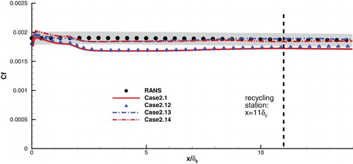
Because the grid resolution of Case 2.1 is sufficient for WRLES, for a deeper analysis in Case 2.12 a WRLES was put up, utilizing the same subgrid-scale model as the aforementioned WMLES. The other numerical settings were the same as Case 2.1. Figure 14 reveals that the Cf error of WRLES is existent and comparable to that of IDDES. The velocity profile and shear stress show a similar trend to Cf and are not exhibited here. These errors of WRLES presented here accord with Kawai, Shankar, and Lele (2010), who revealed that in the simulation of a Mach 3 flat plate boundary layer using WRLES the precision was affected by many factors and even WRLES using the well-known dynamic Smagorinsky model could lead to apparent errors under the conditions examined. This suggests that the problems met by IDDES in these cases may not be ascribed to the issue of hybrid, but rather may be essentially due to the intrinsic difficulty of LES to resolve the inner layer of a supersonic boundary layer: when resolving the inner layer of a supersonic boundary layer, WRLES should be subtly tuned and needs high computational cost, and may be damaged by any faulty factor, including but not limited to numerical resolution. In order to verify this deduction, we sought to acquire accurate results using WRLES. This was fulfilled by simultaneously densifying the grid and using the MPLD scheme (Case 2.13 in Table 3). As shown in Figure 14, the error of Case 2.12 is essentially eliminated in Case 2.13. Thus, next we put up an IDDES simulation (Case 2.14 in Table 3), with all other numerical settings the same as Case 2.13. Figure 14 shows that IDDES under this condition does provide very satisfying results. These results further suggest that, at least for the present supersonic flow cases, IDDES can be capable of precisely predicting skin friction, if and only if under the same condition the relevant LES which uses the same subgrid-scale model can precisely predict skin friction. In other words, the performance of IDDES is closely related to the ability of the relevant LES model in resolving the inner layer.

Figure 14. Comparison of the distributions of the mean friction coefficient Cf of Cases 2.12–2.14 and Case 2.1.

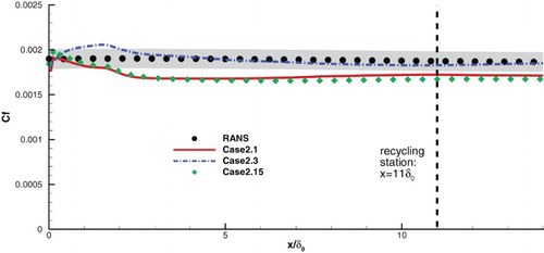
Thus it is not surprising that ZDES and HRLMEC are free from problems because the RANS-to-LES interface of them locates far away from the wall, while that of IDDES is close to the wall. To further verify this, in Case 2.15 we change the RANS-to-LES interface of ZDES to y⁺ = 11, a similar wall-normal location to that of IDDES. Under this condition, the error of ZDES is comparable to that of IDDES, as shown in Figure 15. This further suggests that the problem of underpredicting the mean friction coefficient is existent not only in IDDES, but also in other hybrid RANS/LES methods which locate the RANS-to-LES transition very close to the wall and need to resolve most of the inner layer.

Figure 15. Comparison of the distributions of the mean friction coefficient Cf of Case 2.15, Case 2.1 and Case 2.3.

5. Conclusions

To the authors’ knowledge, this article for the first time conducts a detailed assessment of the prediction of mean skin friction in supersonic boundary layer flows using the WMLES part of the popular IDDES method. In this article, the IDDES method acting as WMLES was used to simulate spatially developing supersonic flat plate boundary layers at two Reynolds numbers, together with another two blending methods, namely ZDES and HRLMEC, for comparison. The underprediction of mean skin friction is existent in the result of IDDES but negligible in the result of ZDES and HRLMEC when all the other settings are identical. This presents a striking contrast to the original idea of IDDES and some former simulations in subsonic flows. With the analysis of the shear stress, we attribute the underprediction of mean skin friction of IDDES to the underprediction of total Reynolds stress and TKE production in the inner layer. Because the RANS-to-LES interface of IDDES is close to the wall, most of the inner layer is simulated using the LES mode, but the resolved Reynolds stress is not sufficient to compensate for the lack of modeled Reynolds stress. The other two blending methods do not suffer from this because the RANS-to-LES interface of them is much further away from the wall. From an additional simulation of WRLES, it can be inferred that the problems met by IDDES may be essentially due to the intrinsic difficulty of LES to resolve the inner layer of a supersonic boundary layer, which should be subtly tuned and may be damaged by any faulty factor. Further research shows that, at least as regards the present supersonic flow cases, IDDES can be capable of precisely predicting skin friction, but only if under the same condition the relevant LES which uses the same subgrid-scale model can precisely predict skin friction. However, the condition is not easily satisfied in complex supersonic flows, so it is against the primary intention of hybrid RANS/LES methods.

The study suggests that special attention must be paid when using IDDES as WMLES, especially if the accurate prediction of skin friction is a focal point. The limitation of the study is that no modification to the IDDES model itself regarding the existing problem has been established. In order to take advantage of the robustness of IDDES for complex supersonic flows while improving the performance in prediction of skin friction, a modification to IDDES is supposed to be beneficial. The modification may be realized by recalibrating the empirical functions and constants, or adjusting the RANS-to-LES transition of WMLES to a position further away from the wall with an elaborate fabrication. This is to be studied in our future investigation.

Disclosure statement

No potential conflict of interest was reported by the authors.

Additional information

Funding

This work was supported by the National Natural Science Foundation of China [grant number 91641107].

Appendix 1. Details of the blending method for the LAM scheme

The LAM scheme is a blend of the MPLD scheme and the adaptive MUSCL scheme through a weighting function : (A.1)

Here u_i+1/2 denotes the flow variable reconstructed at the cell face. The scheme will reduce to the MPLD scheme if and to the adaptive MUSCL scheme if . is obtained using the following procedures. First define an indicator function: (A.2) with ε = 1E^–15 to avoid the numerical overflow when both and are equal to 0 and . Here denotes the cell averaged of the flow variable. The smoothness at the cell face i + 1/2 is defined as the minimum of two adjacent cells given by: (A.3)

A threshold value is selected to obtain weighting coefficient as follows: (A.4) Usually, the parameter is problem dependent. In order to resolve small structures and unsteadiness such as in the LES region, a smaller value of should be chosen to increase the weight in a smooth region. But a smaller value will result in numerical instability for practical cases. In this article, it is fixed to be 0.4.

References

- Billet, G., & Louedin, O. (2001). Adaptive limiters for improving the accuracy of the MUSCL approach for unsteady flows. Journal of Computational Physics, 170, 161–183. doi: 10.1006/jcph.2001.6731
- Choi, H., & Moin, P. (1994). Effects of the computational time step on numerical solutions of turbulent flow. Journal of Computational Physics, 113, 1–4. doi: 10.1006/jcph.1994.1112
- Choi, H., & Moin, P. (2012). Grid-point requirements for large eddy simulation: Chapman's estimates revisited. Physics of Fluids, 24(1), 011702, 1–5. doi: 10.1063/1.3676783
- Choi, J.-I., Edwards, J. R., & Baurle, R. A. (2009). Compressible boundary-layer predictions at high Reynolds number using hybrid LES/RANS methods. AIAA Journal, 47(9), 2179–2193. doi: 10.2514/1.41598
- Cocks, P. A. T., Bruno, C., Donohue, J. M., & Haas, M. (2013). IDDES of a dual-mode ethylene fueled cavity flameholder with an isolator shock train. AIAA Paper, AIAA 2013-0116.
- Deck, S. (2005). Zonal-detached-eddy simulation of the flow around a high-liftconfiguration. AIAA Journal, 43(11), 2372–2384. doi: 10.2514/1.16810
- Deck, S. (2012). Recent improvements in the zonal detached eddy simulation (ZDES) formulation. Theoretical and Computational Fluid Dynamics, 26, 523–550. doi: 10.1007/s00162-011-0240-z
- Deck, S., Renard, N., Laraufie, R., & Sagaut, P. (2014). Zonal detached eddy simulation (ZDES) of a spatially developing flat plate turbulent boundary layer over the Reynolds number range 3150≤Reθ≤14000. Physics of Fluids, 26(2), 025116, 1–32. doi: 10.1063/1.4866180
- Deck, S., Renard, N., Laraufie, R., & Weiss, P. E. (2014). Large scale contribution to mean wall shear stress in high Reynolds number flat plate boundary layers up to Reθ=13650. Journal of Fluid Mechanics, 743, 202–248. doi: 10.1017/jfm.2013.629
- Deck, S., Weiss, P. E., Pamiés, M., & Garnier, E. (2011). Zonal detached eddy simulation of a spatially developing flat plate turbulent boundary layer. Computers & Fluids, 48, 1–15. doi: 10.1016/j.compfluid.2011.03.009
- Edwards, J. R., Choi, J.-I., & Boles, J. A. (2008). Hybrid LES/RANS simulation of a Mach5 compression-corner interaction. AIAA Journal, 46(4), 977–991. doi: 10.2514/1.32240
- Fang, J., Li, Z. R., & Lu, L. P. (2013). An optimized low-dissipation monotonicity-preserving scheme for numerical simulations of high-speed turbulent flows. Journal of Scientific Computing, 56, 67–95. doi: 10.1007/s10915-012-9663-y
- Georgiadis, N. J., Rizzetta, D. P., & Fureby, C. (2010). Large-eddy simulation: Current capabilities, recommended practices, and future research. AIAA Journal, 48(8), 1772–1784. doi: 10.2514/1.J050232
- Gieseking, D. A., Choi, J.-I., Edwards, J. R., & Hassan, H. A. (2011). Compressible-flow simulations using a new large-eddy simulation/Reynolds-averaged Navier-Stokes model. AIAA Journal, 49(10), 2194–2209. doi: 10.2514/1.J051001
- Jameson, A., & Yoon, S. (1986). LU implicit scheme with multiple grid for the Euler equations. AIAA Paper, AIAA 1986-0105.
- Kawai, S., Shankar, S. K., & Lele, S. K. (2010). Assessment of localized artificial diffusivity scheme for large-eddy simulation of compressible turbulent flows. Journal of Computational Physics, 229(5), 1739–1762. doi: 10.1016/j.jcp.2009.11.005
- Krappel, T., Kuhlmann, H., Kirschner, O., Ruprecht, A., & Riedelbauch, S. (2015). Validation of an IDDES-type turbulence model and application to a Francis pump turbine flow simulation in comparison with experimental results. International Journal of Heat And Fluid Flow, 55, 167–179. doi: 10.1016/j.ijheatfluidflow.2015.07.019
- Larsson, J., Kawai, S., Bodart, J., & Bermejo-Moreno, I. (2016). Large eddy simulation with modeled wall-stress: Recent progress and future directions. Mechanical Engineering Reviews, 3, 15-00418–15-00418. doi: 10.1299/mer.15-00418
- Le, J., Yang, S., Liu, W., & Xing, J. (2005). Massively parallel simulations of kerosene-fueled scramjet. AIAA Paper, AIAA 2005-3318.
- Lund, T., Wu, X., & Squires, K. (1998). Generation of turbulent inflow data for spatially-developing boundary layer simulations. Journal of Computational Physics, 140(2), 233–258. doi: 10.1006/jcph.1998.5882
- Menter, F. R. (1994). Two-equation eddy-viscosity turbulence models for engineering applications. AIAA Journal, 32(8), 1598–1605. doi: 10.2514/3.12149
- Menter, F. R., Schütze, J., & Gritskevich, M. (2012). Global vs. zonal approaches in hybrid RANS-LES turbulence modelling. Progress in Hybrid RANS-LES Modelling, Springer Berlin Heidelberg, 15–28.
- Morgan, B., Larsson, J., Kawai, S., & Lele, S. K. (2011). Improving low-frequency characteristics of recycling/rescaling inflow turbulence generation. AIAA Journal, 49(3), 582–597. doi: 10.2514/1.J050705
- Nikitin, N. V., Nicoud, F., Wasistho, B., Squires, K. D., & Spalart, P. R. (2000). An approach to wall modeling in large-eddy simulations. Physics of Fluids, 12(7), 1629–1632. doi: 10.1063/1.870414
- Peterson, D. M., & Candler, G. V. (2011). Simulations of mixing for normal and low-angled injection into supersonic crossflow. AIAA Journal, 49(12), 2792–2804. doi: 10.2514/1.J051193
- Piomelli, U. (2008). Wall-layer models for large-eddy simulations. Progress in Aerospace Sciences, 44(6), 437–446. doi: 10.1016/j.paerosci.2008.06.001
- Pulliam, T. H. (1993). Time accuracy and the use of implicit methods. AIAA Paper, AIAA 1993-3360.
- Renard, N., & Deck, S. (2016). A theoretical decomposition of mean skin friction generation into physical phenomena across the boundary layer. Journal of Fluid Mechanics, 790, 339–367. doi: 10.1017/jfm.2016.12
- Shur, M. L., Spalart, P. R., Strelets, M. K., & Travin, A. K. (2008). A hybrid RANS-LES model with delayed DES and wall-modeled LES capabilities. International Journal of Heat and Fluid Flow, 29, 1638–1649. doi: 10.1016/j.ijheatfluidflow.2008.07.001
- Shur, M. L., Spalart, P. R., Strelets, M. K., & Travin, A. K. (2014). Synthetic turbulence generators for RANS-LES interfaces in zonal simulations of aerodynamic and aeroacoustic problems. Flow, Turbulence and Combustion, 93, 63–92. doi: 10.1007/s10494-014-9534-8
- Strelets, M. (2001). Detached eddy simulation of massively separated flows. AIAA Paper, AlAA2001-087 9.
- Urbin, G., Knight, D., & Zheltovodov, A. (2001). Large eddy simulation of a supersonic boundary layer using an unstructured grid. AIAA Journal, 39(7), 1288–1295. doi: 10.2514/2.1471
- Wang, H. S., Piao, Y., & Niu, J. (2015). IDDES simulation of supersonic combustion using flamelet modeling. AIAA Paper, AIAA 2015-3211.
- Wilcox, D. C. (2006). Turbulence modeling for CFD (3rd ed.). La Canada, CA: Dcw Industries, Incorporated.
- Zhao, M., Zhang, M., & Xu, J. (2017). Numerical simulation of flow characteristics behind the aerodynamic performances on an airfoil with leading edge protuberances. Engineering Applications Of Computational Fluid Mechanics, 11(1), 193–209. doi: 10.1080/19942060.2016.1277165