Numerical investigation of the aerodynamic characteristics of high-speed trains of different lengths under crosswind with or without windbreaks

ABSTRACT

The focus of this study was the influence of the length of a train on its aerodynamic performance, with and without wind break walls, under a crosswind. The improvement in the train’s aerodynamic performance due to a wind break wall was also analyzed. Aerodynamic coefficients such as the drag force and lateral force were obtained for trains of different lengths using a numerical simulation. A delayed detached eddy simulation based on the shear-stress transport κ–ω turbulent model was used in Fluent 14.0 to simulate the unsteady aerodynamic performances of trains of different lengths under a crosswind. Through a comparison and analysis of the simulation results, the effects of the train length on the forces, pressure, and flow structure around the train were studied, along with the influence of a wind break wall on trains of different lengths. The results showed that the effects on the forces, pressure, and flow structure were focused in the region around the train tail. Furthermore, it was found that a wind break wall could improve the aerodynamic characteristics of a train under a crosswind, but amplified the influence of the train length on the aerodynamic performance of the train tail. These research results provide useful guidance for train operations under a crosswind.

KEYWORDS:

• High-speed train
• crosswind
• train length
• windbreaks
• aerodynamic characteristic
• numerical simulation

1. Introduction

The flow around a high-speed train is in a highly unsteady state, and vortex shedding from the train often occurs (Zhang, Li, Tian, Gao, & Sheridan, 2016). This phenomenon is especially significant under a crosswind (Hemida, Krajnovic, & Davidson, 2005). The aerodynamics of a high-speed train may deteriorate in a crosswind, which may even cause the train to tip over. Therefore, the study of the aerodynamic performance of a train under a crosswind has attracted much attention from researchers. A crosswind causes a low-frequency fluctuation in the unsteady aerodynamic force on a train, which is close to the natural frequency of a real train (Hemida & Krajnović, 2006; Liu, Zhang, & Zhang, 2013; Tomasini & Cheli, 2013). In recent years, with the rapid development of computers, some researchers, including Xi, Mao, Gao, and Yang (2014), Hemida and Krajnović (2010), Östh and Krajnović (2014), and Ashton and Revell (2015), have studied the unsteady aerodynamic performance of a train under a crosswind using large eddy simulation (LES), detached eddy simulation (DES), and delayed detached eddy simulation (DDES).

Because a train is composed of several vehicles, its length can be changed to respond to the needs of different transportation requirements. Some researchers have studied the effect of a train’s length on its aerodynamic performance. Tian (2000) performed a wind tunnel test to determine a train’s aerodynamic performance without a yaw angle, and found that the drag on the head car, middle cars, and tail car stopped changing when the number of vehicles in a train was more than five. Riccoa, Baronb, and Moltenib (2007) found that the pressure caused by a longer train, running through a tunnel, was greater and lasted longer than the pressure caused by a shorter train in a moving model test. Huang, Chen, and Jiang (2012) investigated the distribution of the drag on each vehicle in trains with different lengths, without a yaw angle, using a wind tunnel test. It was found that the change in drag on the tail car was small, and the drag on the middle cars changed little when the number of vehicles was more than three. Mao, Yanhong, and Yang (2012) studied the aerodynamic characteristics of trains of different lengths using numerical simulation and established a dimensionless relationship between the train drag and train length. Mao et al. (2012) also found that the method used to evaluate the safety of the head car could be used to evaluate the safety of the whole train and that, while this method is conservative, it is reasonable and feasible. Muld, Efraimsson, and Henningson (2014) studied the flow structures around a train, without a yaw angle, using numerical simulation, and found that increasing the boundary layer thickness of the train decreases the Strouhal number of the most dominant flow structures, and that these structures have different wavelengths. Bell, Burton, Thompson, Herbst, and Sheridan (2015) studied the slipstream and wake of a high-speed train using a moving model test and found that, the shorter the train, the thinner the boundary layer thickness on the train. There are, however, few references discussing the influence of train length on the aerodynamic performance of a train under a crosswind.

Therefore, in this study, the aerodynamic performances of trains of different lengths under a crosswind were investigated. Because a wind break wall is often used to reduce the effects of wind on a train’s aerodynamic performance (Avila-Sanchez, Pindado, Lopez-Garcia, & Sanz-Andres, 2014; Marzok, Deh, Courteille, & Zimmermann, 2007; Tomasini, Giappino, Cheli, & Schito, 2016; Xiang, Li, Wang, & Liao, 2015; Zhang, Xia, & Guo, 2013), the effect of a wind break wall was also analyzed.

This paper is organized as follows. In Section 2, the train model, numerical method, grid, and boundary are introduced. Section 3 introduces the grid independence and Reynolds effects on the train’s aerodynamic performance. The grids, numerical schemes, and boundary conditions used in this study are verified in Section 4. The influences of the train length and wind break wall on the train forces, surface pressure, and flow structure around the train are analyzed in Section 5. Section 6 details the conclusions.

2. CFD analysis

2.1. Methodology

Because the mesh density requirement of Reynolds averaged Navier-Stokes (RANS) models is lower than that for LES, the mesh density in the train’s boundary layer was reduced for DDES. Spalart (2009) considered DDES to be effective for solving a fluid field with a large flow separation, such as the flow field around the train in this study. DDES has been used successfully to simulate the flow field around a train (Ashton & Revell, 2015; Huang, Hemida, & Yang, 2016; Lee, Campbell, & Hambric, 2014). DDES was also used to study the effects of the train length and wind break wall on the unsteady aerodynamic performance of the train. DDES is an improvement on the original DES method of 1997 (Spalart, Jou, Strelets, & Allmaras, 1997), which suffered from grid-induced flow separation. This phenomenon, which is caused by the premature switch between the RANS and LES modes in the exterior region of the boundary layer, has been observed by users. The mesh density could not support the Reynolds stress resolution of the LES in the exterior region of the boundary layer. Therefore, the switch caused a reduced eddy viscosity, an effect known as modeled stress depletion (MSD) (Spalart, Deck, Shur, Squires, Strelets, & Travin, 2006). DDES was used in this study to prevent the occurrence of MSD and premature flow separation. The separation flow and details of the flow field could be better simulated using DDES based on the shear-stress transport (SST) κ–ω turbulent model. In the k–ω turbulent model (Menter, 1994), the κ and ω equations are as follows: (1) (2) where t, ρ, and are the time, air density, and airflow velocity components in the direction, respectively. In this study,  = 0.5 and  = 0.856. The terms , _, and are the blending function, production term, and destruction term for the turbulence kinetic energy equation, respectively.

To avoid grid-induced separation, a shielding function is introduced to act as a second condition to delay the switch inside the boundary layer. is defined as follows (Shur, Spalart, Strelets, & Travin, 2008): (3) where is the length scale in the destruction term of the turbulent kinetic energy κ equation. The term Δ is the LES length scale and is defined as . Consequently, ∼ 0 inside the boundary layer and f_d ∼ 1 far away from the wall. The SST-based DDES model is finally constructed by replacing in the destruction term of the K equation with from the DES model (Krimmelbein & Radespiel, 2009).

The flow region where is close to 0 will be the region where the RANS is functional (i.e. within the boundary layer). The RANS model used for the DDES in the present study was the SST κ–ω two-equation model. The flow region where is equal to 1 will be the region where the LES is functional (i.e. outside the boundary layer).

In this study, a pressure-based solver was used for the simulation. The gradient of the resulting variable at the center of the cell was obtained using the least-squares cell-based method. The semi-implicit method for the pressure-linked equations (SIMPLE) algorithm was used to solve the pressure and velocity coupling equation. The bounded central differencing scheme was used to solve the momentum equation. The second-order upwind scheme was used to solve the κ and ω equations. The time discretization method used the unsteady calculation method of the dual-time step format. The physical time step was 1 × 10⁻⁴s (Hemida & Krajnović, 2008, 2009a), and the number of iterations in each time step was 30. In each time step, the maximum residual of each turbulent equation converged to 10⁻⁵. The lower–upper symmetric Gauss–Seidel (LU-SGS) implicit scheme was used for the time integral, and the second-order implicit scheme was used for the transient formulation.

2.2. Computational model and boundary conditions

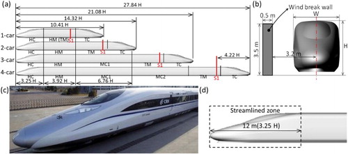
In this study, the CRH380A train model was simplified for the computational model. The bogie region and windshield were omitted. Four lengths (10.41 H, 14.32 H, 21.08 H, and 27.84 H) were used for the train model, as shown in Figure 1(a), to study the effect of the length on the aerodynamic performance of the train. The width (W) and height (H) of the full-scale train model were 3.4 m and 3.7 m, respectively. The details of the train size are also shown in Figures 1(a) and (b). To facilitate the study, the train model was broken down into several parts, as shown in Figure 1(a). As shown in Figure 1(b), there is a gap between the train model and ground surface, and the distance between them is 0.2 m (distance between the upper surface of the track and bottom surface of the train) for the full-scale model. For example, the 1-car train model was composed of HC, HM, TM, and TC, where HC is the streamlined head car, HM is the region between the streamlined head car and second middle car, TM is the region between the streamlined tail car and last middle car, and TC is the streamlined tail car. To calculate the case with windbreaks, the width and height of the cross-section of the full-scale windbreaks were, respectively, 0.5 m and 3.5 m, and the distance between the center of the railway and the leeward side of the windbreaks was 3.2 m, as shown in Figure 1(b).

Figure 1. Train model: (a) different lengths of trains, (b) train cross-section, (c) CRH380A, and (d) streamlined region of train model.

The calculation cases in this study were divided into two types: open air and wind break wall. As listed in Table 1, the open air type included four train lengths (1 car, 2 cars, 3 cars, and 4 cars), and the wind break wall type included three train lengths (1 car, 2 cars, and 3 cars).

Table 1. Calculation cases.

Open air				Wind break wall
C1	C2	C3	C4	C5	C6	C7
1-car	2-car	3-car	4-car	1-car	2-car	3-car

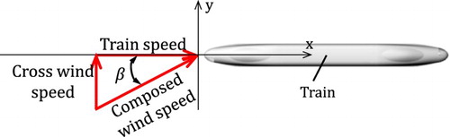
The compound velocity method, which incorporates the wind speed and train speed, is widely used to simulate a train’s aerodynamic characteristics under a crosswind (Baker, 2010; Cheli, Ripamonti, Rocchi, & Tomasini, 2010; Suzuki, Tanemoto, & Maeda, 2003). In this study, the international commercial software Fluent 14.0 was used to solve the flow around the train. Its solutions were based on the finite volume method. The wind speed profile has a large effect on the flow field (Cheli, Corradi, & Tomasini, 2012; Zheng, Zhang, & Gu, 2012), and may interfere with the analysis of the effect of the train length and wind break wall on the aerodynamic performance of a train. However, most of the previous studies, including those of Östh and Krajnović (2014), García, Muñoz-Paniagua, Jiménez, Migoya, and Crespo (2015), and Ashton and Revell (2015), did not consider this effect. Therefore, the effects of the wind speed profile and roughness of the ground were not considered in this study. The mean velocity of the incoming flow, U_m, was 60 m/s, which was composed of the wind speed and train speed, and the yaw angle, β, was 15°, which is defined in Figure 2. The velocity inlet boundary has typically been used to simulate the incoming flow (García et al., 2015; Hemida & Krajnović, 2009b; Morden, Hemida, & Baker, 2015; Wang, Xu, Zhu, & Li, 2014) because it simplifies the method for defining its characteristics. The uniform (and constant in time) velocity profile of U_m was used for the velocity inlet boundary. Both the front face and one side of the computational domain were used to define the velocity inlet boundary, and a component was used to deal with the velocity specification method in the velocity inlet boundary. The component in Fluent 14.0 includes three speed components. In this study, the x-direction (train running direction) was U_msinβ, the y-direction (crosswind direction) was U_mcosβ, and the z-direction was zero. In Fluent 14.0, the turbulent kinetic energy κ and specific dissipation rate ω were selected in the turbulence specification method. These could be calculated using Equations (4) and (5) and had values of 0.54 m²/s² and 41.44 s⁻¹, respectively: (4) (5) where is 60 m/s, I is the turbulence intensity (1% in this study), H is the characteristic length (0.4625 m in this study), and is the empirical constant (0.09 in this study).

Figure 2. Definition of composed wind and yaw angle.

The top face, back face, and remaining side face of the computational domain were defined as the pressure outlet boundary condition, and the reference pressure P_out was 0 Pa. To simulate the relative movement between the wind break wall and the trains and between the ground and the trains, the ground and wind break wall were defined as the slip wall condition, where the slip velocity was the train speed. The boundary of the computational region is defined in Figure 3. The size of the computational domain in this study was greater than that required by the CEN standard (2010). The size details of x and x_T in Figure 3 are listed in Table 2.

Figure 3. Boundary conditions and size of computational region.

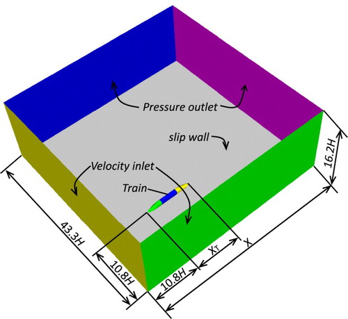
Table 2. Size of computational region.

Value	1-car	2-car	3-car	4-car
xT	10.41 H	14.32 H	21.08 H	27.84 H
x	43.24 H	54.05 H	64.86 H	75.78 H

2.3. Grid generation

The open source CFD toolbox OpenFOAM 2.3.1 was used to generate a hexahedral-dominated mesh around the train, as shown in Figure 4. The train’s flow field was simulated using the pressure-based solver in Fluent 14.0. The numerical simulation used 1:8 scale models. Morden et al. (2015) studied the grid independence with four meshes and found that, for DDES based on an SST κ-ω turbulence model, a mesh of 34 million cells provided the best balance between accuracy and computational cost. The averaged y+ was about 10. Zhang et al. (2016) studied the impact of the ground effect on train aerodynamics with 16 million cells using a DES based on the realizable κ-ε turbulence model. They also obtained good results. The size of the train model was nearly the same as that in case 1 of this paper. Three refinement regions were found around the train, as shown in Figure 4(b). To meet the requirements of the vortex on the leeward side of the train on the grid, the refinement on the leeward side was approximately twice the width of the refinement on the windward side of the train, as shown in Figure 4(c). For example, in case 4, the length, width, and height of the fine box were 35, 1.875, and 0.75 m, respectively, whereas those of the middle box were 15.625, 3.125, and 1.25 m; and those of the coarse box were 26.25, 4.375, and 1.875 m, respectively. The maximum mesh sizes for the fine, middle, and coarse boxes were approximately 7.8, 31.2, and 62.4 mm, respectively. The size of the smallest mesh on the train surface was 1.95 mm, and 10 prism layers were applied to the train surface boundary. The grid generation in the other cases was similar to that of case 4, the only difference among them being the length of the refinement box, which was decreased with decreasing train length. To reduce the mesh number and save computing resources, a wall function was used in the simulation. The thickness of the first boundary layer was approximately 0.195 mm, and the adaptive mesh technique in Fluent 14.0 was used in this numerical simulation to ensure that the averaged y+ was approximately 10, which met the demands of the κ-ω turbulence model (Fluent User's Guide, 2011). To verify the grid independence, four different mesh numbers for C1 were compared: the details of the differences between the four cases are listed in Table 3. The sizes of the refinement boxes in the four cases were the same. The meshes around the train for the different types of grid refinement are shown in Figure 5.

Figure 4. Computational mesh around train: (a) global view, (b) side view, and (c) front view.

Figure 5. Mesh around trains in C1-1, C1-2, C1-3, and C1-4.

Table 3. Details of four cases.

Items	C1-1	C1-2	C1-3 (C1)	C1-4
Number of volume meshes	12,115,886	18,340,014	22,952,612	30,167,442
Size of the smallest mesh on train surface/mm	3.91	1.95∼3.91	1.95	1.95
Number of prism layers	10	10	10	15
Thickness of the first boundary layer/mm	0.391	0.195∼0.391	0.195	0.195
Maximum mesh size in fine, middle and coarse refinement box/mm	15.6, 31.2, 62.4	15.6, 31.2, 62.4	7.8, 31.2, 62.4	7.8, 15.6, 62.4

2.4. Post-processing

2.4.1. Coefficients of force and pressure

The drag and lateral force on a train are significantly affected by shedding vortices. Therefore, two main representative aerodynamic forces were selected to describe the influences of the train length and wind break wall on the aerodynamic performance of the train. According to the CEN standard (2013), some coefficients are defined as follows: (6) (7) (8) where is the drag force, is the lateral force, and p is the static pressure on the train surface. C_d is the drag coefficient, is the lateral force coefficient, is the pressure coefficient, and is the reference pressure, which is 0 Pa. The air density parameter ρ is equal to 1.225 kg/m³, and reference area S is equal to 0.15625 m².

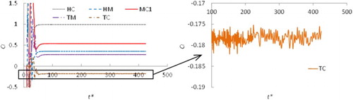
2.4.2. Mean quantities and vortex visualization technique

The flow around a train is turbulent. The train aerodynamic coefficients are in a state of fluctuation over time. Based on the literature (Hemida & Krajnović, 2008; Zhang et al., 2016), the non-dimensional time ‘t* = tU_m/H’ was used to process the unsteady quantities, and the size of the time step in non-dimensional time units Δt* = ΔtU_m/H = 0.01297. The lateral force on the train for C3 is shown in Figure 6. The drag, lateral force, and other quantities are then calculated by taking the average value over the non-dimensional time t* from 90 (t = 0.70 s) to 272 (t = 2.1 s), which is sufficient for calculating the mean quantities (Hemida & Baker, 2010; Hemida & Krajnović, 2010; Östh & Krajnović, 2014).

Figure 6. Time history curves of C_l of train for case 3.

The iso-surface of the constant Q is used to describe the transient vortex structure and has been widely used in describing the flow structure around a train (Flynn, Hemida, Soper, & Baker, 2014; Zhang et al., 2016). The value of Q is given by the following: (9) where u_i,j and u_j,i are the velocity gradient tensors.

3. Grid independence and Reynolds effects

3.1. Grid independence

This section discusses how the C1 train model (Table 1) was used as the model for the numerical simulation in the test cases to determine the grid independence and Reynolds number effect, with C1-3 used for the grid independence test cases (C1-1, C1-2, C1-3, and C1-4). The differences between C1-1, C1-2, C1-3, and C1-4 were the density and grid number. The boundary conditions of the computational domain in the grid independence test cases (C1-1 to C1-4) and the Reynolds number effect test cases were similar to those in C2 to C7 (Figure 3). As listed in Table 4, both the C_d and C_l values of the train, except the HC, decreased with an increase in the grid number, while the C_l value of the HC increased. When the grid number reached 2.30E + 07, the aerodynamic forces on the train changed very little, by no more than 1%. Therefore, a grid size of 2.30E + 07 (C1-3) was suitable for this calculation.

Table 4. Average aerodynamic force coefficients of 1-car train in four cases.

	Cd			Cl
Case	HC	HM (TM)	TC	HC	HM (TM)	TC
C1-1	−0.1009	0.0538	0.1609	1.0734	0.3237	−0.1419
C1-2	−0.0990	0.0525	0.1546	1.0896	0.3285	−0.1667
C1-3	−0.0981	0.0517	0.1516	1.1044	0.3379	−0.1786
C1-4	−0.0979	0.0516	0.1518	1.1043	0.3380	−0.1777

3.2. Reynolds effects

As listed in Table 5, the mean C_l of the TC increased with an increase in the Reynolds number, but the mean C_l and C_d of the other train parts decreased. The Reynolds number can be calculated as follows: (10) where U_m was 20 m/s, 60 m/s, or 80 m/s. The term ρ is the air density, which was 1.225 kg/m³. The coefficient η is the dynamic viscosity coefficient, and was 1.83 × 10⁻⁵ Pa·s.

Table 5. Average C_d and C_l values of trains with different Reynolds numbers.

	Cd			Cl
Reynolds number	HC	HM (TM)	TC	HC	HM (TM)	TC
6.33E + 05	−0.0768	0.0644	0.1523	1.1430	0.4100	−0.1456
1.90E + 06	−0.0974	0.0515	0.1516	1.1044	0.3379	−0.1777
2.54E + 06	−0.1007	0.0498	0.1514	1.1013	0.3249	−0.1824

The relationship between the aerodynamic force coefficient and the Reynolds number was the same as the relationship in the reference (Östh & Krajnović, 2014). When the Reynolds number reached 1.90E + 06, the aerodynamic forces on the train changed relatively little, by no more than 5%. Therefore, the Reynolds number chosen for all of the cases in this study was 1.90E + 06.

4. Comparison of experiment and numerical simulation results

In order to verify the reliability of the calculations presented in this paper, an algorithm validation was carried out. At present, we only have data from a test performed in a wind tunnel using a 1:8 scale two-car (head car + tail car) train of CRH380A with a bogie and windshield (Niu, Liang, & Zhou, 2016; Niu, Zhou, & Liang, 2017). The model used in the wind tunnel test was somewhat different from the one used in this calculation. However, we can compare the pressures on the head car surface from the calculation and wind tunnel test to improve the reliability of the numerical calculation method used in this paper, considering that the flow around the head car was not affected by the train length.

4.1. Model and grids

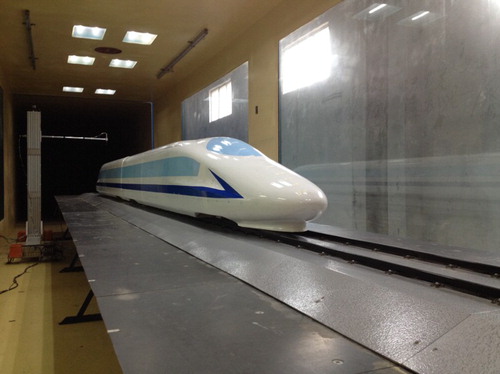
The train model used in this simulation was the 1:8 scale 1-car train in C1 (Figure 1(a)). The computational domain was similar to that of the 1-car train in Figure 3 and Table 2. The 1:8 scale model used in the wind tunnel test comprised two cars (Figure 7). The streamlined head car used in the wind tunnel was similar to that in the numerical simulation.

Figure 7. Train model in wind tunnel.

The mesh density of C1-3 in Section 3.1 was used to generate the computational domain mesh in this simulation. The smallest mesh size on the train surface, number of prism layers, and thickness of the first boundary layer were 1.95, 10, and 0.20 mm, respectively. The grid around the train is shown in C1-3 in Figure 5.

4.2. Numerical schemes

This section discusses a simulation that was conducted to verify the rationality of the numerical schemes used in this study. The DDES based on the SST κ–ω turbulent model was also used in this simulation. The other settings and parameters were similar to those discussed in Section 2.1.

4.3. Boundary conditions

Figure 3 shows the boundary conditions of the computational domain used in this numerical simulation. The data from the wind tunnel test were obtained using a flow field of 60 m/s, turbulence intensity of 0.3%, and yaw angle of 15°. The experiments were performed in the high-speed test section of the wind tunnel in the National Engineering Laboratory for High-Speed Railway Construction, Central South University (Niu et al., 2016, 2017). The characteristics of the incoming flow velocity in this numerical simulation were made similar to those of the wind tunnel test using Equations (4) and (5) to eliminate the effects of the Reynolds number and interference from other factors.

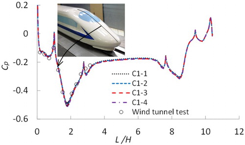
4.4. Comparison and analysis

A comparison of the aerodynamic forces could not be carried out because of the absence of a train model with bogies in the numerical simulation. Instead, a comparison of the aerodynamic pressure on the streamlined head car was carried out. To ensure the quality of the observed data, both the wind tunnel test and numerical simulation were carried out under a crosswind with a sideslip angle of 15°. Figure 8 shows that the surface pressure distribution on the head car in the wind tunnel test is consistent with the surface pressure distribution in the numerical simulation. Moreover, a small difference in the pressure amplitudes is found.

Figure 8. Data comparison between experiment and numerical simulation.

5. Results and analysis

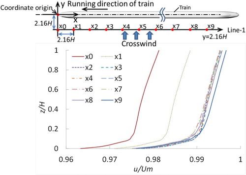
The wind speed profile on the windward side of the train is shown in Figure 9. Figure 9 also shows that the wind speed profiles in the region downstream of point x2 on line 1 (y = 2.16H) are very close, which means that the effect of the differing wind speed profiles on the flow around the train is concentrated in the region before point x2. The influence of the train length on the aerodynamic performance of the train is, therefore, not significantly affected by the wind speed profile.

Figure 9. Wind speed profile on windward side of train.

5.1. Aerodynamic force analysis

5.1.1. Analysis of mean aerodynamic force coefficients

The results listed in Table 6 show that, when the train length increased without a wind break wall, the mean C_d values of TM and TC decreased, and the decrease in the mean C_d for TC was 26.5%, which was the most significant mean C_d decrease, whereas the decreases in the mean C_d values for other parts of the train were no more than 3.3%. The results listed in Table 6 also show that the mean C_d of each part in a train was significantly affected by the wind break wall, and had no relationship between the train length and mean C_d value for cases with a wind break wall.

Table 6. Mean C_d of each part in train.

		Mean Cd
		Head car				Tail car
Condition	Case	HC	HM	MC1	MC2	TM	TC	Total mean Cd
Open air	C1	−0.09798	∖	∖	∖	0.05148	0.15232	0.10582
	C2	−0.09635	0.05092	∖	∖	0.05139	0.12849	0.13445
	C3	−0.09576	0.05121	0.08786	∖	0.05038	0.11738	0.21107
	C4	−0.09522	0.05084	0.08746	0.08503	0.04978	0.11196	0.28985
Wind break wall	C5	−0.19434	∖	∖	∖	0.05861	0.23146	0.09573
	C6	−0.19200	0.05745	∖	∖	0.05367	0.25734	0.17646
	C7	−0.18856	0.05731	0.08875	∖	0.04957	0.18503	0.19209

The results listed in Table 7 show that the mean C_l values of TM and TC were significantly affected by the length of the train, and for the open air condition, the maximum C_l values of TM and TC were 38.48% and 43.97%, respectively, whereas the changes in the mean C_l values for other parts of the train were no more than 3%. The results listed in Table 7 also show that both the direction and amplitude of the lateral force of each part in a train were changed by the wind break wall, and, for the cases with a wind break wall, there was no specific relationship between the train length and the mean C_l values for other parts of the train. However, the mean C_l values for most parts of the train were decreased by the wind break wall.

Table 7. Mean C_l of each part in train.

		Mean Cl
		Head car				Tail car
Condition	Case	HC	HM	MC1	MC2	TM	TC	Total mean Cl
Open air	C1	1.11044	∖	∖	∖	0.33794	−0.17865	1.26973
	C2	1.12040	0.39931	∖	∖	0.30740	−0.16145	1.66566
	C3	1.11776	0.39847	0.60523	∖	0.30839	−0.20102	2.22882
	C4	1.12557	0.40914	0.62397	0.58744	0.20789	−0.28815	2.66586
Wind break wall	C5	−0.31492	∖	∖	∖	−0.27865	−0.45223	−1.04580
	C6	−0.30934	−0.18815	∖	∖	−0.59331	−0.14726	−1.23805
	C7	−0.30674	−0.18252	−0.67320	∖	0.04879	0.01712	−1.09655

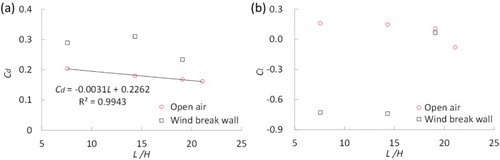
Figure 10(a) shows that the mean drag coefficient of the tail car without a wind break wall has a linear relationship with the train length. However, with the wind break wall, the mean drag coefficients of the HM and TC are affected by the train length, with maximum changes of 45.82% and 41.83%, respectively. For the other parts, the change is no more than 3%, as listed in Table 6. The mean drag coefficient of the tail car with a wind break wall does not have a linear relationship with the train length. Figure 10(b) shows that the wind break wall significantly amplifies the influence of the train length on the mean lateral force coefficients of TM and TC, with maximum changes of 91.78% and 96.21%, respectively, whereas, for the other parts, the change is no more than 2.7%, as listed in Table 5. Figure 10(b) also shows that the lateral force direction on the tail car changed without a wind break wall, when the train length reached 21.09 H, corresponding to C4. The wind break wall decreased the train’s lateral force when the train length reached 19.09 H, corresponding to C6, and the lateral force direction of the tail car changed.

Figure 10. Time averaged drag and lateral force coefficients of tail car variation with train length.

5.1.2. Analysis for SD of aerodynamic force coefficients

Standard deviation (SD) is employed to evaluate the fluctuation degree of aerodynamic coefficients (Daniels, Castro, & Xie, 2016; Niu et al., 2017; So, Wang, Xie, & Zhu, 2008). The formula used to calculate the SD is defined as follows: (11) where σ is the standard deviation (SD); N is the number of samples; is an individual sample; the subscript i shows the order of the sample data, which ranges from 1 to N; and μ is the average of the samples.

The SD values of the drag coefficient and lateral force coefficient for all cases are presented in Tables 8 and 9, respectively. The values listed in Tables 8 and 9 show that there is no obvious regular relationship between the train length and the SD values of C_d and C_l for each part of the train, with or without windbreaks. However, the windbreaks increased the SD values of C_d and C_l for most parts of the train, which meant the windbreaks exacerbated the fluctuations of C_d and C_l for most parts of the train, especially for the train’s tail. Comparing the SD values of C_d and C_l listed in Tables 8 and 9, it was found that the fluctuation of C_d is smaller than that of C_l for most parts of the train.

Table 8. SD of drag coefficient of each part in train.

		Cd
		Head car				Tail car
Condition	Case	HC	HM	MC1	MC2	TM	TC	Total Cd
Open air	C1	1.70E-05	∖	∖	∖	3.35E-07	6.72E-04	6.89E-04
	C2	3.05E-07	4.45E-04	∖	∖	5.43E-10	2.10E-07	4.46E-04
	C3	4.93E-04	6.44E-07	1.15E-09	∖	8.78E-07	2.39E-07	4.95E-04
	C4	1.69E-06	3.55E-10	1.99E-07	4.19E-04	3.02E-09	7.47E-07	4.22E-04
Wind break wall	C5	7.94E-05	∖	∖	∖	1.70E-05	4.13E-04	5.09E-04
	C6	6.70E-05	1.36E-05	∖	∖	1.72E-05	2.63E-04	3.61E-04
	C7	9.16E-05	1.65E-05	1.87E-05	∖	1.78E-05	9.28E-04	1.07E-03

Table 9. SD of lateral force coefficient of each part in train.

		Cl
		Head car				Tail car
Condition	Case	HC	HM	MC1	MC2	TM	TC	Total Cl
Open air	C1	2.74E-05	∖	∖	∖	5.48E-05	2.11E-03	2.19E-03
	C2	1.26E-05	2.42E-03	∖	∖	2.24E-08	6.26E-05	2.50E-03
	C3	1.60E-03	4.73E-05	8.42E-08	∖	2.86E-06	1.70E-05	1.67E-03
	C4	1.43E-04	2.01E-08	1.13E-05	4.18E-03	2.54E-07	7.44E-06	4.34E-03
Wind break wall	C5	3.32E-05	∖	∖	∖	5.72E-05	2.20E-03	2.29E-03
	C6	2.93E-04	7.66E-04	∖	∖	6.81E-04	1.59E-03	3.34E-03
	C7	7.27E-04	3.76E-03	1.29E-06	∖	1.06E-03	1.29E-03	6.84E-03

5.2. Influence of train length and wind break wall on flow field around a train

5.2.1. Impact of train length

5.2.1.1. Flow structure analyses

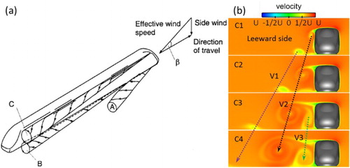
Figure 11(a) shows a schematic view of the flow structures around a train for small and moderate yaw angles. There are three large and long shedding vortices (A, B, and C) on the leeward side of the train. Vortex A comes from the lower leeward edge of the leading nose and rapidly flows away from the train body. Vortex C emerges from the upper leeward edge of the leading nose, and is closer to the train body than vortex A. Vortex B is generated from the train bottom and grows steadily along the train under vortex C. Vortices B and C are always close to the train. This phenomenon has been observed in the studies of Khier, Breuer, and Durst (2000), Hemida and Krajnović (2010), and García et al. (2015). The S1 in the different cases is a cross-section, which is a distance of 4.22 H from the nose of the train tail, as shown in Figure 1. In Figure 11(b), vortices V1, V2, and V3 correspond to vortices A, C, and B, respectively, in Figure 10(a). More detailed information about these three vortices can be obtained in Figure 10(b). Figure 11(b) shows that there is a significant flow structure difference on the leeward sides of trains with different lengths. Vortex V1 is always close to the ground and interacts with the ground, which gradually weakens its intensity. Vortex V2 moves down as the train length increases, and its influence increases markedly. The low velocity of the flow on the leeward side of the train causes V2 to rotate counterclockwise. This phenomenon also appeared in the study of Cheli et al. (2010). When the train length reaches a certain value, such as in the C3 condition, the third vortex, V3, appears on the leeward side of the train. As the train length increases, V3 slowly moves away from the train, but its strength and size gradually increase. Limited by vortex V2, the height of V3 is basically unchanged, and its rotation is clockwise.

Figure 11. Flow structure around train: (a) schematic view of flow structures around train for small and moderate yaw angles (Khier et al., 2000) and (b) mean velocity contour of S1 (see Figure 1) variation with train length.

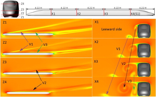
As shown in Figure 12, the flow structure around the train in the C3 condition contains all the vortices. Therefore, C3 is taken as an example to describe the flow structure around the train. Comparing the different cross-sections of the flow structures shown in the right picture of Figure 12, the position and regularity of the development of the vortices V1, V2, and V3 on the leeward side of the train are both confirmed. V1 is formed by the combined effect of the airflow coming from the train’s front cowcatcher and the airflow coming from the train’s bottom. V2 is formed by the interaction of the airflow on the train’s leeward side and the airflow flowing from the train’s top. V3 is formed by the interaction of the airflow on the train’s leeward side and the airflow from the train’s bottom. The left picture of Figure 12 shows that, when the height of a section increases, the wake intensity decreases. In other words, the wake is mainly located in the region below the train nose.

Figure 12. Mean velocity contours in horizontal and vertical sections for C3: Z1 = 0.11 H, Z2 = 0.22 H, Z3 = 0.43 H, and Z4 = 0.86 H.

Figure 13(a) shows the instantaneous flow structures around the train in C3. Four main vortices are found around the leeward side of the train, while many vortices are generated around the head and tail cars. A greater number of vortices leads to a more turbulent flow. The flow around the head and tail cars is more turbulent than the flow around the middle cars. Flow separation occurs most often on the upper surface of the streamlined head and tail cars and the cowcatcher of the head car. Thus, the fluctuation of the aerodynamic forces is more marked for the head and tail cars than for the middle cars.

Figure 13. Instantaneous iso-surface plot of Q-criteria collared by mean velocity U (Q = 50,000): (a) flow structure in C3 and (b) different train lengths.

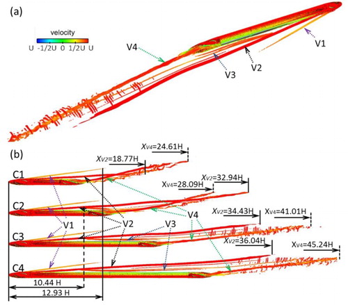
As shown in Figure 13(a), both of the detached vortices, V1 and V2, are produced from the head car. Thus, the train length does not affect the positions from which V1 and V2 are shed. As shown in Figure 13(b), V1 disappears at a distance of 12.93 H from the train nose, which indicates that the train length does not affect the position at which V1 disappears. In C1, C2, C3, and C4, V2 disappeared at 18.77 H, 32.94 H, 34.43 H, and 36.04 H, respectively, which indicates that the increase in the train length led to an increase in the length of V2 and also accelerated its dissipation. V3 was shed from the train at a distance of 10.44 H from the train nose, which indicated that the position from which V3 was shed was not affected by the train length. With the development of V3, its intensity gradually weakened and it merged with V4. As shown in Figure 13(a), V4 is shed from the train tail. As shown in C1 and C2, V4 goes across V2 at a position that moves downstream with an increase in the train length. When the train length is more than 21.08 H (the length of the train in C3), V4 no longer goes across V2, which causes the position at which V4 disappears to move downstream. In addition, in C1, C2, C3, and C4, V4 disappears at 24.61 H, 28.09 H, 41.01 H, and 45.24 H, respectively, as shown in Figure 13(b). Comparing the dissipation positions of V2 and V4, C2 is different from the others, with the dissipation of V4 earlier than that of V2, whereas the dissipation of V4 is later than that of V2 in the other three cases. This is an interesting phenomenon, which could be studied in more depth in the future.

5.2.1.2 Train surface pressure analyses

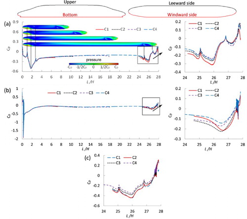
With an increase in train length, the vortices were further from the train, and the thickness of the boundary layer on the train increased. These characteristics mainly concerned the flow field around the train. However, the pressure on the train could be influenced by the change in the flow structure on it. The pressure distribution on the centerline of the train, in Figure 14, shows why an increase in train length causes the drag on the tail car to decrease and the lateral force on the tail car to increase (see Figure 10). As shown in the pressure contours of Figure 14(a), the pressure distribution on the train’s top surface is not affected by the train length, most of the area is a negative pressure area, and the area around the tail car nose is essentially at a positive pressure. From the distribution of C_p along the train in Figures 14(a) and 14(b), a difference is apparent in the area around the nose of the train tail. C_p on the upper surface of the train tail has the largest value for C1, followed by C2, C4, and C3. The causes of this phenomenon may include the fact that the train length in C1 is shorter than in the others, and the reduction effect of the boundary layer of the train on the velocity of the airflow is relatively small, which leads to the airflow separation on the windward side of the tail car being relatively greater. Therefore, the negative pressure on the windward side of the tail car would be relatively larger. The train tail surface pressure below the train nose is the largest for C2, followed by C1, C3, and C4. Figure 14(c) shows that the train length does not affect the phenomenon whereby the surface pressure of the streamlined tail car is in a state of negative pressure. Figure 14(c) also shows that the negative pressure is larger for C1 and C2, followed by C3 and then C4, corresponding to the regular drag listed in Table 6.

Figure 14. Distributions of mean C_p along length of train: (a) upper, (b) bottom, and (c) sum of upper and bottom.

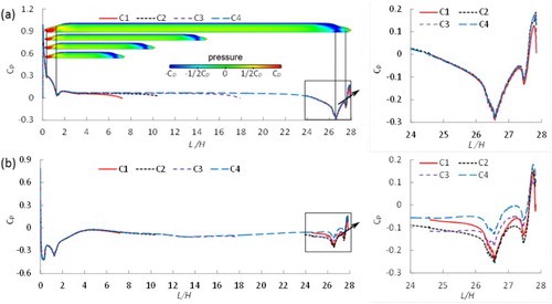
As shown in Figure 15(a), for trains of different lengths, the windward side of the nose of the head car is at a large positive pressure, and the airflow is separated from the windward side of the streamlined tail car, which leads to the appearance of a larger negative pressure in this area. The train length has hardly any effect on the distribution regularity and amplitude of the pressure on the windward side of the train. Figure 15(a) shows that a big difference in the pressure amplitude appears around the nose of the tail car. This difference may be caused by the vortices shedding from the train nose. C_p in C1 is a little larger than in the other cases, for the negative pressure on the windward side of the tail car, and the causes of this phenomenon may be the same as depicted in Figure 14(a): the airflow separation on the windward side of the tail car is relatively larger for the shorter train. Figure 15(b) shows that the main difference in the pressure distributions along the train’s leeward side for trains of different lengths appears mainly in the region of the train tail, with C2 having the largest negative pressure, followed by C1, C3, and C4. The train lateral force under a crosswind is mainly caused by the pressure difference between the windward and leeward sides. In addition, the negative pressure on the windward side of the tail car is greater than that on the leeward side. Therefore, the lateral force on the tail car is the largest for C4, followed by C3, C1, and C2, which is consistent with the distribution regularity values listed in Table 7.

Figure 15. Distributions of mean C_p along length of train: (a) windward side and (b) leeward side.

5.2.2. Effect of wind break wall

5.2.2.1. Flow structure analyses

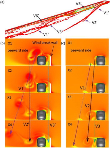
The instantaneous flow structures around the train in C7 are shown in Figure 16(a). There are six main vortices around the leeward side of the wind break wall. Among these, vortices V1′, V2′, V4′, and V5′ are generated by the wind break wall, whereas V6′ is caused by the nose of the tail car. Additional small vortices appear behind the train, caused by the interaction among the trailing vortex and vortices separated from the wind break wall. Figure 16(b) shows the vortex location and its coverage: the farther V1′ is from the head car nose in the vertical direction, the farther it is from the train body in the lateral direction. The location of V2′ is essentially unchanged. With an increase in the vortex length, vortex V3′, located between the train body and the wind break wall, is stronger. This phenomenon appeared in the studies of Xiang et al. (2015). Compared to the velocity distributions shown in Figures 16(b) and 16(c), the velocity of the flow in the upper portion of the leeward side of the train with a wind break wall is higher than that of a train without a wind break wall, which reflects the accelerating effect of the wind break wall on the airflow located in the upper portion of the leeward side of the train. The wind break wall decreases the number of shedding vortices on the leeward side of the train, and draws these shedding vortices away from the train more quickly, but also produces a vortex between the wind break wall and the train. This vortex interacts with the train, together with the vortices on the leeward side of the train, to decrease the lateral force on the train.

Figure 16. Flow field around train with wind break wall: (a) instantaneous vortex structure around train in C7, (b) velocity distribution around train with different cross-sections for C7, and (c) velocity distribution around train with different cross-sections for C3.

5.2.2.2 Train surface pressure analyses

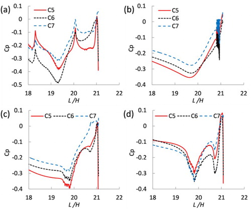
With the wind break wall, the pressure distributions on the head and middle cars along the train still do not appear to differ among different train lengths. Nevertheless, a difference appears in the area around the train tail. Figure 17 shows that wind not only amplifies the differences in the surface pressure distributions along the tail car, among trains of different lengths, but also increases the negative pressure around the tail car. The airflow, separating from the top of the wind break wall, affects the tail car, and also disturbs the regularity of the pressure distribution along the tail car, among the three cases. The windward side pressure on the tail car with the wind break wall decreased as the train length increased, which may have been due to the decay of the detached vortex V3′. The wind break wall did not change the trend for the pressure distribution with the train length on the tail car bottom and leeward side; it only increased their negative pressure amplitudes.

Figure 17. Distributions of mean C_p along train in vertical plane: (a) upper, (b) bottom, (c) windward side, and (d) leeward side.

5.3. Effect of turbulence on train aerodynamic performance

As listed in Table 10, the total mean C_d and C_l values of the 1-car train were decreased by an increase in the turbulence intensity, but the decreases were less than 0.25%. When the turbulence intensity increased, the mean C_d of HM (TM) increased, mean C_d of other parts decreased, and mean C_l of each part of the 1-car train increased. This was because the air separation around HC and TC was suppressed by the high turbulence intensity, according to the boundary layer theory (Schlichting, 1979). This phenomenon was also observed in the wind tunnel test of Cheli, Corradi, Sabbioni, and Tomasini (2011) and Cheli, Giappino, Rosa, Tomasini, and Villani (2013). The results listed in Table 6 also show that the influence of the turbulence on the aerodynamic forces of TC was the largest.

Table 10. Mean C_d and C_l values of each part in 1-car train in flow fields with different turbulence intensities.

	Mean Cd				Mean Cl
Item	HC	HM (TM)	TC	Total mean Cd	HC	HM (TM)	TC	Total mean Cl
Tu = 1%	−0.09744	0.05148	0.15162	0.10566	1.10446	0.33794	−0.17778	1.26462
Tu = 2.62%	−0.09596	0.05233	0.14902	0.10540	1.10578	0.33908	−0.18312	1.26174
Difference/%	−1.52	1.66	−1.71	−0.25	0.12	0.34	3.00	−0.23

The results listed in Table 11 show that the fluctuation of the aerodynamic forces of TC was the largest among the parts in a train for turbulence intensities of 1% and 2.62%. As shown by the results listed in Table 11, with an increase in the turbulence intensity, the SD values of C_d and C_l, respectively, decreased and increased. This phenomenon was also found by Niu et al. (2017). Comparing the data listed in Table 11 shows that the effect of the turbulence intensity on the fluctuations of C_d for the middle part of the train and C_l for the train tail were the largest.

Table 11. SD values of C_d and C_l for each part in 1-car train in flow fields with different turbulence intensities.

	Cd				Cl
Item	HC	HM (TM)	TC	Total Cd	HC	HM (TM)	TC	Total Cl
Tu = 1%	1.70E-05	3.35E-07	6.72E-04	6.89E-04	2.74E-05	5.48E-05	2.11E-03	2.19E-03
Tu = 2.62%	1.65E-05	2.79E-07	6.44E-04	6.61E-04	2.88E-05	5.83E-05	2.40E-03	2.49E-03
Difference/%	−2.67	−16.67	−4.13	−4.10	5.20	6.44	13.75	13.46

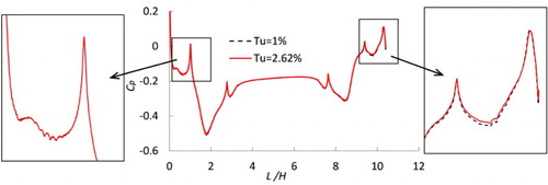
The pressure coefficient of the train’s upper surface is shown in Figure 18. This shows that the pressure distribution along the train is not affected by the turbulence intensity, but the effect of the turbulence intensity on the surface pressure of the train tail is greater than the surface pressure of other regions of the train. Figure 18 also shows that the negative pressure on the train tail is increased by an increase in the turbulence intensity, and this phenomenon was also found by Cheli et al. (2011, 2013) and Niu et al. (2017). Turbulence of 1% and 2.62% had almost no effect on the pressure on both sides of the train. In other words, the flow field in the upper part of the train tail was most easily affected by the turbulence.

Figure 18. Distributions of mean C_p along upper surface of 1-car train in flow fields with different turbulence intensities.

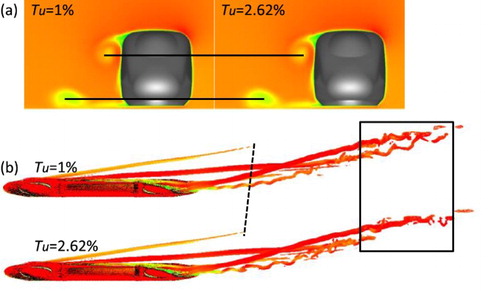
The black line in Figure 19(a) shows that the positions of the main vortices around the 1-car train are not affected by the turbulence intensity. Both the black dotted line and black box shown in Figure 19(b) demonstrate that a large turbulence intensity accelerates the dissipation of vortex V1 and the wake vortices, which means the vortex strength is decreased by an increase in the turbulence intensity.

Figure 19. Flow fields with different turbulence intensities around 1-car train: (a) mean velocity contour of S1 (see Figure 1) and (b) instantaneous vortex structure around train.

5.4 Effect of the bogie on the aerodynamic performance of the train

Table 12 shows that the HC and TC of Cd are increased by the bogie, but the Cl of the HC and TC are decreased. This indicates that the bogie significantly alters the aerodynamics for the part of the train with which it is associated. As shown in the table, the distribution rule for the aerodynamic forces at different parts of the train is not changed by the bogie.

Table 12. Average aerodynamic force coefficients of a 1-car train with or without bogies.

	Cd			Cl
Bogie	HC	HM (TM)	TC	HC	HM (TM)	TC
Without	−0.1009	0.0538	0.1609	1.0734	0.3237	−0.1419
With	−0.2323	0.0462	0.3797	0.9662	0.3193	−0.1269

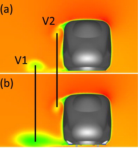
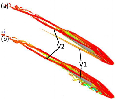
Figure 20 shows that the position and region of the vortex V2 around the train (with and without bogie) are nearly identical, but the region of the vortex V1 around the train with the bogie is greater than without the bogie. This indicates that the bogie mainly affects the flow structure around the bottom of the train.

Figure 20. Distribution of velocity around the train: (a) without bogie and (b) with bogie.

The three-dimensional vortices V1 and V2 are shown in Figure 21, and indicate that V1 around the train is significantly affected by the bogie, which presents a strong pulsation. The reason for the aforementioned phenomenon is that vortex V1 is formed by the interaction of vortices between the cowcatcher and the bogie, with the vortex from the bogie attenuating the vortex from the cowcatcher. The wake is not significantly affected by the bogie.

Figure 21. Instantaneous iso-surface plot of Q-criteria collared by mean velocity U (Q = 50,000): (a) without bogie and (b) with bogie.

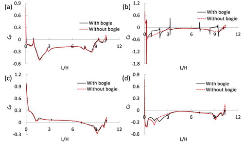
Figure 22 also shows that the pressure on the bottom and leeward side of the train are influenced by the bogie more than the upper and windward side of the train. The distribution of pressure along the train is not changed by the bogie. As seen in Figures 22(a) and (b), the major pressure difference on the bottom of the train appears in the bogie region, with the first bogie having the largest impact on the train’s surface pressure.

Figure 22. Distributions of mean C_p along length of a 1-car train: (a) upper, (b) bottom, (c) windward side, and (d) leeward side.

6. Conclusions

The flow fields of trains of different lengths (10.41 H to 27.84 H) were simulated with and without a wind break wall, and the following conclusions were drawn:

1. Regardless of whether there was a wind break wall, the forces on the tail car, relative to other parts of the train, were significantly affected by the train length. Without the wind break wall, increasing the train length increased the drag on the tail car but decreased the lateral force. The relationship between the drag on the tail car and the train length was linear, and, when the train length was greater than 20.81 H, the direction of the lateral force on the tail car changed. With the wind break wall, increasing the train length decreased the drag on the tail car but increased the lateral force. When the train length was more than 20.81 H, the direction of the lateral force on the tail car also changed.

2. There was no obvious regular relationship between the train length and the SD values of C_d and C_l for each part of the train, with or without windbreaks. However, the windbreaks exacerbated the fluctuations of C_d and C_l for most parts of the train, especially for the train’s tail. The C_d fluctuations for most parts of the train were smaller than those of C_l for most parts of the train.

3. For the cases without windbreaks, the position at which V1 disappeared was not affected by the train length. An increase in the train length led to an increase in the length of V2, and also accelerated the dissipation of V2. In addition, the position from which V3 was shed was not affected by the train length. With the development of V3, its intensity gradually weakened and it merged with V4.

4. More small vortices appeared behind the train, caused by the interaction of the trailing vortex and vortices separated from the wind break wall. The wind break wall decreased the number of shedding vortices on the leeward side of the train and drew these shedding vortices away from the train more quickly, but also produced a vortex between the wind break wall and the train. This vortex interacted with the train, together with the vortices on the leeward side of the train, to decrease the lateral force on the train.

5. The train length mainly affected the flow structure around the train tail, especially the vortex on the leeward side of the train, and the wake. The airflow separating from the train tail caused the tail to be effectively in a state of negative pressure.

6. For the other parts of the train, the surface pressure on the tail car was mainly influenced by the train length. Without the wind break wall, the top, bottom, and leeward side pressures on the tail car were significantly influenced by the train length. With the wind break wall, the pressure around the tail car was also clearly affected by the train length, and the wind break wall amplified this effect.

7. For a turbulence of less than 2.62%, with an increase in the turbulence intensity, the mean C_d of HM (TM) increased, mean C_d of other parts decreased, and mean C_l of each part of the 1-car train increased. In addition, the SD values of C_d and C_l respectively decreased and increased.

It should be noted that the present work utilized the compound velocity method, the train model used in this work was simplified, and the effects of bogies and the windshield were not considered. Future studies will mainly focus on simulated cases that are closer to real conditions, such as through the use of slip mesh technology and by considering the influences of the wind speed profile and roughness of the ground.

Acknowledgments

Finally, we thank the engineers at the Beijing Computing Center, who assisted us in completing the calculations and provided the license for using the Fluent 14.0 software.

Disclosure statement

No potential conflict of interest was reported by the authors.

Additional information

Funding

This work was sponsored by the National Natural Science Foundation of China (grant numbers U1534210, U1334205, and 11372360); the Hunan Provincial Innovation Foundation for Postgraduates (grant number CX2015B046); the Science Technology Research Programme of China Railway Corporation (grant number 2016T004-A and 2016T004-C); the Project of Innovation-driven Plan in Central South University (grant number 2015CX003); and the Natural Science Foundation of Hunan Province (grant numbers 14JJ1003 and 14JJ3028).

References

- Ashton, N., & Revell, A. (2015). Key factors in the use of DDES for the flow around a simplified car. International Journal of Heat and Fluid Flow, 54, 236–249. doi: 10.1016/j.ijheatfluidflow.2015.06.002
- Avila-Sanchez, S., Pindado, S., Lopez-Garcia, O., & Sanz-Andres, A. (2014). Wind tunnel analysis of the aerodynamic loads on rolling stock over railway embankments: The effect of shelter windbreaks. Vascular and Endovascular Surgery, 2014(6), 488–494.
- Baker, C. J. (2010). The simulation of unsteady aerodynamic cross wind forces on trains. Journal of Wind Engineering and Industrial Aerodynamics, 98(2), 88–99. doi: 10.1016/j.jweia.2009.09.006
- Bell, J. R., Burton, D., Thompson, M. C., Herbst, A. H., & Sheridan, J. (2015). Moving model analysis of the slipstream and wake of a high-speed train. Journal of Wind Engineering and Industrial Aerodynamics, 136, 127–137. doi: 10.1016/j.jweia.2014.09.007
- CEN European Standard. (2010). Railway applications–aerodynamics. Part 6: Requirements and test procedures for cross wind assessment, CEN EN 14067-6.
- CEN European Standard. (2013). Railway applications – aerodynamics. Part 4: Requirements and Test Procedures for Aerodynamics on Open Track, CEN EN 14067-4.
- Cheli, F., Corradi, R., Sabbioni, E., & Tomasini, G. (2011). Wind tunnel tests on heavy road vehicles: Cross wind induced loads—part 1. Journal of Wind Engineering and Industrial Aerodynamics, 99(10), 1000–1010. doi: 10.1016/j.jweia.2011.07.009
- Cheli, F., Corradi, R., & Tomasini, G. (2012). Crosswind action on rail vehicles: A methodology for the estimation of the characteristic wind curves. Journal of Wind Engineering and Industrial Aerodynamics, 104–106, 248–255. doi: 10.1016/j.jweia.2012.04.006
- Cheli, F., Giappino, S., Rosa, L., Tomasini, G., & Villani, M. (2013). Experimental study on the aerodynamic forces on railway vehicles in presence of turbulence. Journal of Wind Engineering and Industrial Aerodynamics, 123, 311–316. doi: 10.1016/j.jweia.2013.09.013
- Cheli, F., Ripamonti, F., Rocchi, D., & Tomasini, G. (2010). Aerodynamic behaviour investigation of the new EMUV250 train to cross wind. Journal of Wind Engineering and Industrial Aerodynamics, 98(4), 189–201. doi: 10.1016/j.jweia.2009.10.015
- Daniels, S. J., Castro, I. P., & Xie, Z.-T. (2016). Numerical analysis of freestream turbulence effects on the vortex-induced vibrations of a rectangular cylinder. Journal of Wind Engineering and Industrial Aerodynamics, 153, 13–25. doi: 10.1016/j.jweia.2016.03.007
- Fluent Inc. (2011). Fluent user’s guide. Lebanon, NH: Fluent Incorporated.
- Flynn, D., Hemida, H., Soper, D., & Baker, C. (2014). Detached-eddy simulation of the slipstream of an operational freight train. Journal of Wind Engineering and Industrial Aerodynamics, 132, 1–12. doi: 10.1016/j.jweia.2014.06.016
- García, J., Muñoz-Paniagua, J., Jiménez, A., Migoya, E., & Crespo, A. (2015). Numerical study of the influence of synthetic turbulent inflow conditions on the aerodynamics of a train. Journal of Fluids and Structures, 56(9), 134–151. doi: 10.1016/j.jfluidstructs.2015.05.002
- Hemida, H., & Baker, C. (2010). Large-eddy simulation of the flow around a freight wagon subjected to a crosswind. Computers and Fluids, 39(10), 1944–1956. doi: 10.1016/j.compfluid.2010.06.026
- Hemida, H., & Krajnovic, S. (2006, September 5–8). Numerical study of the unsteady flow structures around train-shaped body subjected to side winds. ECCOMAS CFD 2006: Proceedings of the European conference on computational fluid dynamics. Egmond aan Zee, The Netherlands, Delft University of Technology; European Community on Computational Methods in Applied Sciences (ECCOMAS).
- Hemida, H., & Krajnović, S. (2008). LES study of the influence of a train-nose shape on the flow structures under cross-wind conditions. Journal of Fluids Engineering, 130(9), 253–257. doi: 10.1115/1.2953228
- Hemida, H., & Krajnović, S. (2009a). Transient simulation of the aerodynamic response of a double-deck bus in gusty winds. Journal of Fluids Engineering, 131(3), 031101. doi: 10.1115/1.3054288
- Hemida, H., & Krajnović, S. (2009b). Exploring flow structures around a simplified ICE2 train subjected to a 30° side wind using LES. Engineering Applications of Computational Fluid Mechanics, 3(1), 28–41. doi: 10.1080/19942060.2009.11015252
- Hemida, H., & Krajnović, S. (2010). LES study of the influence of the nose shape and yaw angles on flow structures around trains. Journal of Wind Engineering and Industrial Aerodynamics, 98(1), 34–46. doi: 10.1016/j.jweia.2009.08.012
- Hemida, H., Krajnovic, S., & Davidson, L. (2005, June). Large eddy simulations of the flow around a simplified high speed train under the influence of cross-wind. Proceedings of 17th AIAA computational dynamics conference, Toronto, Ontario, Canada.
- Huang, S., Hemida, H., & Yang, M. (2016). Numerical calculation of the slipstream generated by a CRH2 high-speed train. Proceedings of the Institution of Mechanical Engineers, Part F: Journal of Rail and Rapid Transit, 230(1), 103–116. doi: 10.1177/0954409714528891
- Huang, Z. X., Chen, L., & Jiang, K. L. (2012). Influence of length of train formation and vestibule diaphragm structure on aerodynamic drag of high speed train model. Journal of Experiments in Fluid Mechanics, 26(5), 36–41.
- Khier, W., Breuer, M., & Durst, F. (2000). Flow structure around trains under side wind conditions: A numerical study. Computers and Fluids, 29(2), 179–195. doi: 10.1016/S0045-7930(99)00008-0
- Krimmelbein, N., & Radespiel, R. (2009). Transition prediction for three-dimensional flows using parallel computation. Computers and Fluids, 38(1), 121–136. doi: 10.1016/j.compfluid.2008.01.004
- Lee, A. H., Campbell, R. L., & Hambric, S. A. (2014). Coupled delayed-detached-eddy simulation and structural vibration of a self-oscillating cylinder due to vortex-shedding. Journal of Fluids and Structures, 48, 216–234. doi: 10.1016/j.jfluidstructs.2014.02.019
- Liu, J. L., Zhang, J. Y., & Zhang, W. H. (2013). Study on characteristics of unsteady aerodynamic loads of a high-speed train under crosswinds by large eddy simulation. Journal of the China Railway Society, 35(6), 13–21.
- Mao, J., Yanhong, X. I., & Yang, G. (2012). Numerical analysis on the influence of train formation on the aerodynamic characteristics of high-speed trains under crosswind. China Railway Science, 33(1), 78–85.
- Marzok, C., Deh, B., Courteille, P. W., & Zimmermann, C. (2007). Crosswind stability of high-speed train on a high embankment. Proceedings of the Institution of Mechanical Engineers Part F: Journal of Rail & Rapid Transit, 221(2), 205–225. doi: 10.1243/0954409JRRT126
- Menter, F. R. (1994). Two-equation eddy-viscosity turbulence models for engineering applications. Aiaa Journal, 32(8), 1598–1605. doi: 10.2514/3.12149
- Morden, J. A., Hemida, H., & Baker, C. J. (2015). Comparison of rans and detached eddy simulation results to wind-tunnel data for the surface pressures upon a class 43 high-speed train. Journal of Fluids Engineering, 137(4), 041108. doi: 10.1115/1.4029261
- Muld, T. W., Efraimsson, G., & Henningson, D. S. (2014). Wake characteristics of high-speed trains with different lengths. Proceedings of the Institution of Mechanical Engineers Part F: Journal of Rail and Rapid Transit, 228(4), 333–342. doi: 10.1177/0954409712473922
- Niu, J. Q., Liang, X. F., & Zhou, D. (2016). Experimental study on the effect of Reynolds number on the aerodynamic performance of high speed train with and without yaw angle. Journal of Wind Engineering and Industrial Aerodynamics, 157, 36–46. doi: 10.1016/j.jweia.2016.08.007
- Niu, J.-Q., Zhou, D., & Liang, X.-F. (2017). Experimental research on the aerodynamic characteristics of a high-speed train under different turbulence conditions. Experimental Thermal and Fluid Science, 80, 117–125. doi: 10.1016/j.expthermflusci.2016.08.014
- Östh, J., & Krajnović, S. (2014). A study of the aerodynamics of a generic container freight wagon using large-eddy simulation. Journal of Fluids and Structures, 44(1), 31–51. doi: 10.1016/j.jfluidstructs.2013.09.017
- Riccoa, P., Baronb, A., & Moltenib, P. (2007). Nature of pressure waves induced by a high-speed train travelling through a tunnel. Journal of Wind Engineering and Industrial Aerodynamics, 95(8), 781–808. doi: 10.1016/j.jweia.2007.01.008
- Schlichting, H. (1979). Boundary layer theory [M].
- Shur, M. L., Spalart, P. R., Strelets, M. K., & Travin, A. K. (2008). A hybrid rans-les approach with delayed-des and wall-modelled LES capabilities. International Journal of Heat and Fluid Flow, 29(6), 1638–1649. doi: 10.1016/j.ijheatfluidflow.2008.07.001
- So, R. M. C, Wang, X. Q., Xie, W. C., & Zhu, J. (2008). Free-stream turbulence effects on vortex-induced vibration and flow-induced force of an elastic cylinder. Journal of Fluids and Structures, 24(4), 481–495. doi: 10.1016/j.jfluidstructs.2007.10.013
- Spalart, P. R. (2009). Detached-eddy simulation. Annual Review of Fluid Mechanics, 41(1), 181–202. doi: 10.1146/annurev.fluid.010908.165130
- Spalart, P. R., Deck, S., Shur, M. L., Squires, K. D., Strelets, M. K., & Travin, A. (2006). A new version of detached-eddy simulation, resistant to ambiguous grid densities. Theoretical and Computational Fluid Dynamics, 20(3), 181–195. doi: 10.1007/s00162-006-0015-0
- Spalart, P. R., Jou, W. H., Strelets, M., & Allmaras, S. R. (1997). Comments on the feasibility of LES for wings, and on a hybrid RANS/LES approach. Advances in DNS/LES, 1, 4–8.
- Suzuki, M., Tanemoto, K., & Maeda, T. (2003). Aerodynamic characteristics of train/vehicles under cross winds. Journal of Wind Engineering and Industrial Aerodynamics, 91(1–2), 209–218. doi: 10.1016/S0167-6105(02)00346-X
- Tian, H. Q. (2000). Influence of form of train formation on running air resistance. Electric Drive for Locomotive, 2000(4), 9–11.
- Tomasini, G., & Cheli, F. (2013). Admittance function to evaluate aerodynamic loads on vehicles: Experimental data and numerical model. Journal of Fluids and Structures, 38(3), 92–106. doi: 10.1016/j.jfluidstructs.2012.12.009
- Tomasini, G., Giappino, S., Cheli, F., & Schito, P. (2016). Windbreaks for railway lines: Wind tunnel experimental tests. Proceedings of the Institution of Mechanical Engineers Part F: Journal of Rail & Rapid Transit, 405(6790), 1049–1052.
- Wang, B., Xu, Y.-L., Zhu, L.-D., & Li, Y.-L. (2014). Crosswind effect studies on road vehicle passing by bridge tower using computational fluid dynamics. Engineering Applications of Computational Fluid Mechanics, 8(3), 330–344. doi: 10.1080/19942060.2014.11015519
- Xi, Y., Mao, J., Gao, L., & Yang, G. (2014). Aerodynamic force/moment for high-speed train bogie in crosswind field. Journal of Central South University, 45(5), 1705–1715.
- Xiang, H., Li, Y., Wang, B., & Liao, H. (2015). Numerical simulation of the protective effect of railway wind barriers under crosswinds. International Journal of Rail Transportation, 3(3), 151–163. doi: 10.1080/23248378.2015.1054906
- Zhang, J., Li, J.-j., Tian, H.-q., Gao, G.-j., & Sheridan, J. (2016). Impact of ground and wheel boundary conditions on numerical simulation of the high-speed train aerodynamic performance. Journal of Fluids and Structures, 61(4), 249–261. doi: 10.1016/j.jfluidstructs.2015.10.006
- Zhang, T., Xia, H., & Guo, W. W. (2013). Analysis on running safety of train on bridge with wind barriers subjected to cross wind. Wind & Structures An International Journal, 17(2), 203–225. doi: 10.12989/was.2013.17.2.203
- Zheng, D.-Q., Zhang, A.-S., & Gu, M. (2012). Improvement of inflow boundary condition in large eddy simulation of flow around tall building. Engineering Applications of Computational Fluid Mechanics, 6(4), 633–647. doi: 10.1080/19942060.2012.11015448