Accuracy and comparison of standard k-ϵ with two variants of k-ω turbulence models in fluvial applications

ABSTRACT

Racetrack flumes are established experimental settings in ecohydraulics and sediment studies. Their experimental results are often coupled with numerical simulations. The two-equation turbulence closures of the Reynolds-Averaged Navier-Stokes equations are applied widely in such engineering applications. They are preferred for their ease of use and low computational costs compared with more sophisticated turbulence models involving large-scale fluvial simulations. Here, three variants of two-equation models, i.e. the standard k-ϵ model and two variants of k-ω models, were applied to tackle mean flow and turbulence in a racetrack flume and a river reach. Regarding model performances, we found an overall reasonable agreement between simulated and measured mean velocity values. Nonetheless, the simulated turbulent kinetic energy exhibited discrepancies to the measured values. The computational costs of all investigated model variants are comparable. Therefore, there is no significant preference among models. The findings confirm the application of these model approaches for mean flow-related investigations (e.g. habitat modeling) but suggest exercising caution for applications sensitive to turbulent processes.

KEYWORDS:

• Racetrack flume
• two-equation closure
• RANS
• turbulent kinetic energy
• field experiments
• computational expenses

1. Introduction

Humans have long attempted to adapt fluvial networks to their requirements. With every intervention, we not only enhanced our understanding of such systems but also discovered new problems. The inherent complexities call for a reliable understanding of the physical processes and mechanisms for river investigations, regardless of the affordable computational capacity. Currently, simulations of the complex flow fields are already feasible for moderate sizes of flow domains and within relatively simple geometries. In the future, large-scale simulations and their corresponding complex morphological interactions will also become feasible. The increase in computational capacity over the past decades, however, has led to a tendency not to question the results of numerical simulations. Due to the lack of investigations on complex hydraulic processes, it is often disregarded that extensions of straight flow turbulence models must be applied to secondary flows with caution and sufficient validation (Abad & Garcìa, 2009; Blanckaert & De Vriend, 2005).

Racetrack flumes are well-established experimental setups for hydrobiological and ecological studies (Beaulieu, Sengco, & Anderson, 2005; Harii & Kayanne, 2002; Nowell, Jumars, Self, & Southard, 1989) as well as for investigations on water pollution (Wang, Hu, Wang, & Lei, 2015), sedimentology and sediment deposition (Larsen, Harvey, & Crimaldi, 2009; Schieber, 2016; Schieber, Southard, & Thaisen, 2007). The respective results are usually applied to large-scale hydro-systems. Transferring racetrack flume results to fluvial ecosystems is common practice; this is often done using a numerically simulated flow field.

Considering engineering economics, numerical simulations are cost-effective solutions to investigate large-scale fluvial processes. Natural stream simulations are usually based on finding a stable solution for the Reynolds-Averaged Navier-Stokes (RANS) equations. To overcome the closure problem of RANS momentum equations, several turbulence methods have been proposed. Two-equation models, such as the k-ϵ and k-ω models, have become a de facto industrial standard and are widely applied engineering tools. Even though these models have been available for some time, they continue to be a focus of active research (Asnaashari, Akhtari, Dehghani, & Bonakdari, 2016; Fu, Uddin, & Curley, 2016; Nieto, Hargreaves, Owen, & Hernández, 2015; Peralta, Parente, Balogh, & Benocci, 2014; Rudra Reddy & Durbin, 2013; Tritthart, Mayrhofer, Glas, Glock, & Habersack, 2015). In theory these models can be applied to all turbulent flows. In practice, however, they show significant deviations from experimental data when used to model flows involving severe pressure gradients, separation zones and strong streamline curvature (Menter, 1994). Nonetheless, compared with more sophisticated numerical models, e.g. Large Eddy Simulation (LES) or Direct Numerical Simulation (DNS), they have the benefit of significantly lower computational costs. In order to overcome certain shortcomings of the k-ϵ model (e.g. boundary layer inaccuracy in adverse pressure gradients), the classical k-ω model was suggested by Wilcox (1988). Researchers have subsequently modified, applied and discussed different approaches to the k-ω turbulence closure (Fuhrman, Dixen, & Jacobsen, 2010; Goldberg & Batten, 2015; Khosronejad, Rennie, Salehi Neyshabouri, & Townsend, 2007; Menter, 1994; Menter, Ferreira, Esch, & Konno, 2003; Nieto et al., 2015). The classical k-ω model (Wilcox, 1988) received an update (Wilcox, 2008) that added a cross-diffusion term and modified the built-in stress limiter. This significantly enhanced both boundary layer and free surface simulations, as well as decreased the intrinsic sensitivity of k-ω models to shear flows.

In the current study, we apply the RSim-3D software, i.e. a steady state RANS solver based on the finite volume method that operates on arbitrary polyhedral cells (Tritthart, 2005), to compare three different turbulence models by simulating an open racetrack flume. The solver can either neglect (i.e. rigid-lid assumption) or calculate free surface variations. The position of the free surface is obtained from repeatedly translating the pressure surplus or deficit at all near-surface cells into elevation changes. Therefore the model calculates water flow only, i.e. without an additional air phase. Pressure–velocity coupling is performed using the SIMPLE method (Ferziger & Péric, 2002). The second-order upwind scheme is employed for the convective terms and the viscous terms are handled with central differences. The details of the numerical method are given in Tritthart and Gutknecht (2007). RSim-3D is established software for river research and has been widely applied, including for validation with field measurements (e.g. Schludermann, Tritthart, Humphries, & Keckeis, 2012; Tritthart & Gutknecht, 2007; Tritthart, Liedermann, & Habersack, 2009). Successful application of the model in sediment transport studies (Liedermann, Tritthart, & Habersack, 2013; Tritthart, Schober, & Habersack, 2011) and in habitat modeling (Hauer, Unfer, Tritthart, Formann, & Habersack, 2011; Lechner et al., 2014) of natural river reaches raised the question whether racetrack flume experimental results are applicable without restriction to natural streams using conventional numerical models. The answer must consider the strong flow three-dimensionalities (e.g. secondary currents of different kinds) that are inherent to natural streams.

In order to upscale the corresponding results to natural streams, the natural flow field must be resolved using a numerical simulation. The reliability of such generalizations and possible limitations are not usually well investigated. The current study addresses these limitations based on a series of numerical simulations using the conventional turbulence models that are often applied in the context of fluvial studies. Concerning the framework, three turbulence models are investigated: one standard k-ϵ model and two variants of the k-ω model, the latter specially implemented for the current study. In order to obtain a general perspective of encountered numerical complexities and to analyze model performances, the results are compared with experimental data of a racetrack flume (Farhadi, Tritthart, Glas, & Habersack, 2014) as well as with a series of field investigations (Lechner et al., 2014; Tritthart, Glas, Liedermann, & Habersack, 2014). We also compare the computational cost of the different models. Finally, we discuss the results and draw conclusions for future research.

2. Turbulence models and numerical implementation

Fluid motion for incompressible flow is governed by the Navier-Stokes equations in three spatial dimensions. Introducing mean flow and fluctuating quantities into the Navier-Stokes equations yields the Reynolds equations for turbulent flow (see Versteeg & Malalasekera, 2007). The two-equation models investigated here use the Boussinesq approximation, which relates the Reynolds stresses to the mean rates of deformation (Tritton, 1977).

The well-known classical turbulence closure (Launder & Spalding, 1974) was implemented in the RSim-3D solver as the default turbulence model. The corresponding turbulent energy and its dissipation rate formulations are given in Tritthart (2005) and Tritthart and Gutknecht (2007).

Wilcox (1988) assessed the original closure approximations for the class of two-equation models and proposed the model. In 2008, Wilcox re-evaluated the model and suggested an improved variant. The new model (referred to as the improved model in the following) had two new features: an additional cross-diffusion term and a modified built-in stress limiter. Prior to Wilcox, the addition of cross-diffusion to the equation was suggested as a solution for the classical model’s sensitivity to the freestream value of (specific rate of dissipation). This method was reported to be well applicable to wall-bounded flows (Hellsten, 2005; Kok, 2000). Without using a stress limiter, the Boussinesq approximation leads to unrealistic turbulence energy levels, therefore in order to limit Reynolds stresses an alternative formulation for turbulent viscosity was proposed by Wilcox (2008).

3. Boundary conditions

For the described models, four different cases must be considered in terms of boundary conditions: free surface; inlet; outlet; and solid wall boundaries.

3.1. Free surface

The free surface is implemented as a symmetry boundary which means that no fluxes occur across this boundary (i.e. the normal velocity is, therefore, zero at the boundary). All other properties take boundary values equal to those encountered in the cell centroid right beneath the free surface. Ferziger and Péric (2002) noted that a free surface boundary condition of k (turbulent kinetic energy, aka. TKE) and ϵ (turbulent dissipation rate) is appropriate; on the other hand, turbulent structures can be observed exactly at the free surface of a water body. Since no scalar fluxes occur concerning the quantities, the condition of zero fluxes of k and ϵ was used in this work.

The pressure at the free surface is evaluated by using the pressure gradient obtained via the gradient computation approach as described in Tritthart and Gutknecht (2007). This implies that the pressure is not zero at the surface (except for a single outlet surface cell which serves as pressure reference and where it is thus fixed). The resulting extra pressure head can be directly used to locate and subsequently update the position of the free surface.

3.2. Inlet

For the turbulence model the inlet boundary is calculated based on an approach adopted from Versteeg and Malalasekera (2007), using (1) to obtain the turbulent kinetic energy for the bed at the inlet nodes. From the bed to the surface a linear decrease of turbulent kinetic energy is prescribed at the inlet. Therein, is wall shear stress, the density, and empirical constant  = 0.09. Moreover, the dissipation rate for the inlet nodes is calculated from (2) using the previously calculated values for and estimating L as the water depth.

For the models, the established approach is to use the same model as for and apply a relation between and . The standard model relationship for , in combination with , yields (3) which, combined with Equations (1) and (2), provides an inlet boundary condition equation for models.

3.3. Outlet

For outlets a zero gradient boundary in streamwise direction is applied to all quantities. (4) where n is a normal vector to the outlet surface.

3.4. Solid walls

At walls all velocities are set to zero and there are no convective fluxes through the wall. However, since the model does not integrate the governing equations through the wall, several procedures are employed to solve these equations. The grid nodes closest to the wall (near-wall nodes) are located at half the cell height of the flexible user-defined mesh. Hence, the model user is responsible to employ a reasonably fine (dimensionless length) for the calculations, defined as (5) where y is the node distance to the wall and the shear velocity, which is the square root of over the density; denotes the wall shear stress in the turbulent boundary layer and is defined as (6) where is velocity at the grid node and u⁺ the dimensionless velocity (). The corresponding equations of the ‘law of the wall’ are provided by Nezu and Nakagawa (1993) in detail. Based on the relation provided by Versteeg and Malalasekera (2007), the governing equation for the turbulent kinetic energy receives an additional source term (7) where V denotes the cell volume. The dissipation value at the near-wall nodes is assigned as (8) where is the von Karman constant. Initially, a small starting value for k is assigned for use in equation (8); the values of k in the near-wall nodes and in the entire flow domain, as well as in all non-near-wall cells are then permanently updated during the iteration cycles of the model by the solution of the respective governing equations. The momentum equations receive sink terms based on the shear stress at the wall.

As for the classical and improved models, Wilcox (2008) proposed (9) where is a variable defined by non-dimensional surface roughness; the presented boundary condition is for implementation directly at the wall and thus requires near-wall refinement. In RSim-3D this requirement is avoided by the use of wall functions and combining Equations (2) and (3), which yields (10) The criteria for using wall functions is based on the definition (Equation 5); assuming the near-wall cell is in the turbulent region, the wall shear stress is calculated from Equation (6). After the wall shear stress has been obtained, the sink term for the momentum equations reads (11) where is the row of the wall tangential vector that points into the direction of j, and denotes the surface area the cell shares with the wall.

4. Experimental studies

4.1. Racetrack flume study

An experimental study was conducted in a Styrofoam racetrack flume at the Hydraulic Engineering Laboratory of the University of Natural Resources and Life Sciences, Vienna (Farhadi et al., 2014). The racetrack experiment is not directly a part of the current study, although the measurements are used to verify the simulations. The flume consists of two bends with a radius of curvature of 1.25 m and a 2 m-long straight course (Figures 1a and b); the water depth was constant for all runs (0.195 ± 0.005 m). In the experiment, a belt-drive induced flow in a straight part of the flume. Three-dimensional instantaneous velocity measurements were made over 18 cross-sections using an Acoustic Doppler Velocimeter (ADV) device (sampling frequency: 50 Hz) for three different Froude numbers. The Froude number range was selected for maximum similarity with natural rivers. The position of the measured profiles, a typical trapezoidal cross-section (C1-90 to C2-90) and the measurement grid are presented in Figure 1(c). The measurement grid was selected such that boundary proximities and water surface fluctuations were avoided. Regarding the data quality and experimental uncertainties, a detailed discussion is provided by Farhadi et al. (2017). Hydraulic properties of the racetrack flume are presented in Table 1.

Figure 1. Racetrack flume and investigated cross-sections: (a) isometric view of the physical model; (b) 3D view of the belt-drive; (c) plan of the flume, inset: the cross-section of C1-90 to C2-90, measurement points and selected columns I, II, III.

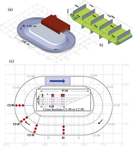
Table 1. Hydraulic properties of the experimental studies.

		Q	U			u*	Rh
Test run		(l s^−1)	(m s^−1)	Re	Fr	(m s^−1)	(m)	R/B	R/H	B/H
	F – 5	9.9	0.067	0.76×10^4	0.05	0.009
	F – 8	14.5	0.098	1.11×10^4	0.08	0.014	0.12	1.69	6.25	3.69
Racetrack	F – 16	29.1	0.197	2.23×10^4	0.16	0.032
Witzelsdorf		2269×10^3	2.05	734×10^4	0.09	0.027	3.66	—	—	—
U = channel mean velocity ()					Q = channel discharge
R = Radius (1.25 m), B = Width, H = Depth (0.20 m)					Re = Reynolds number
Rh = hydraulic radius of C1-90 to C2-90					Fr = Froude number
u* = shear velocity (obtained from the mean velocity distribution in conjunction					H (depth) = 0.195 ± 0.005 m (racetrack)
with the logarithmic law)					= 5.05 (Witzelsdorf measurements)
					B = Channel width

4.2. Field measurements

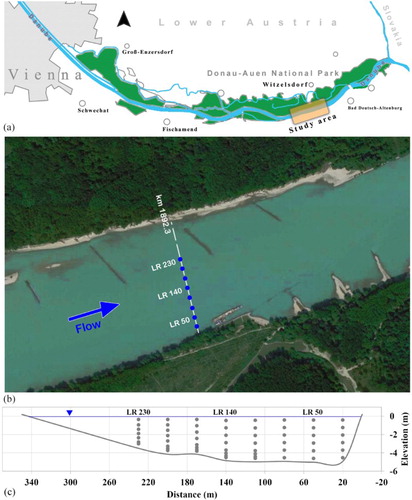
In addition, data series from a river restoration project, which was reported previously in a separate study by Tritthart et al. (2014), were applied for further investigations. The study area comprises a 3 kilometer free-flowing section of the Danube River within the Danube Riparian Zone National Park east of Vienna, Austria. The measurement site is located south of Witzelsdorf village, where alternative groyne layouts were applied to the river channel. Based on the comprehensive field measurements and regarding the data quality and technical concerns, the cross-section at river km 1892.3 was selected in order to be applied to the current work. Three-dimensional instantaneous velocity components in eight columns were measured using an ADV device mounted on a boat. The measured cross-section quantities are presented in Table 1; maximum depth and width of the channel are 5.05 m and 350 m, respectively. The locations of the study area and measurement points, as well as the measurement grid, are depicted in Figure 2. Note that while the river reach is straight, the groyne fields cause highly complex flows including secondary flow.

Figure 2. Witzelsdorf experimental studies (a) location of study area, (b) measurement points, (c) the measurement grid.

5. Results and discussion

5.1. Grid independence test

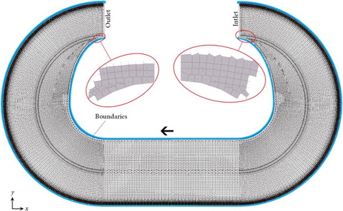
Prior to comparing the different turbulence models, we investigated the sensitivity of the solution to the grid size. This excludes a potential influence of the grid in the subsequent comparison of results. The grid independence test (GIT) determines the optimum grid spacing in order to avoid either excessive refinement or loss of flow details due to a coarse grid size. In order to provide a systematic analysis and based on the procedure suggested by Roache (1998), three computation grids of the racetrack flume were utilized for this test: (1) the standard grid (O); (2) a three-dimensional 20% finer (O+ 20); and (3) a 20% coarser grid (O-20). Evidently, in the region of large gradients (i.e. boundary layers), a finer grid spacing and more grid points are needed to resolve the flow (Figure 3). The first near-wall grid point was set to y⁺ = 12.5 (i.e. centroid cell point) and two points are within the boundary layers for all GIT runs. The rigid-lid and free surface calculations differ by less than 1 millimeter; however, for the sake of precision the free surface calculation is applied. A summary of properties of the different grids applied for the GIT is provided in Table 2. In all simulations reported here, a few grid cells in two small zones close to the inlet and outlet were blocked in the solver, i.e. no fluid flow was allowed through these cells (Figure 4). This was necessary because these cells represent an increasingly steeper wall, causing non-homogeneous deformations that result in numerical artefacts and divergence of the solution. The blocking is imposed only to the half-depth of flow (bed to mid-depth).

Figure 3. Vertical discretization of a typical trapezoidal cross-section of the racetrack flume, comparison columns I, II, III are indicated.

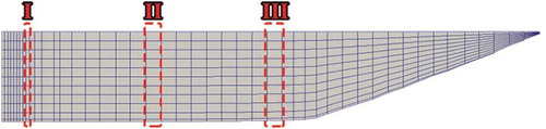
Table 2. Properties of grids.

Grid^a	Grid count (plane × depth)	Average elements dimension Length × Width × Height (m)	Maximum skewness	Average aspect-ratio	y^+ of the first grid point	Element types
Standard (O)	18366 × 11	0.0390 × 0.0250 × 0.0180	0.32	1.83	12.5	Polyhedron with quadrilateral base
Finer (O+ 20)	22359 × 12	0.0312 × 0.0200 × 0.0144	0.34	1.85	12.5	Polyhedron with quadrilateral base
Coarser(O-20)	14607 × 10	0.0468 × 0.0300 × 0.0216	0.41	1.91	12.5	Polyhedron with quadrilateral base

^aUnstructured grids.

Figure 4. Top view of the racetrack flume simulation mesh; the locations of the blocked cells are highlighted.

Based on the experimental measurement plan (Figure 1c), four cross-sections (S3, C2-20, C2-55 and C2-90) and three columns in each (columns I, II, III labeled in Figure 1c: inset and Figure 3) were selected as reference locations. The comparison points were selected to represent all possible domains of flow (i.e. straight and curved courses, locations near banks and the centerline). The GIT was run with the classical model only because, due to the similar nature of all turbulence models considered in this paper, the result should be independent of the model. The results of the GIT for mean streamwise velocity and turbulent kinetic energy (TKE) are presented in Figures 5 and 6, respectively.

Figure 5. Grid independency test for streamwise mean velocity parameter over four cross-sections and three columns; -x- values corresponding to the standard grid (O), • 20% finer grid (O+ 20), O 20% coarser grid (O-20).

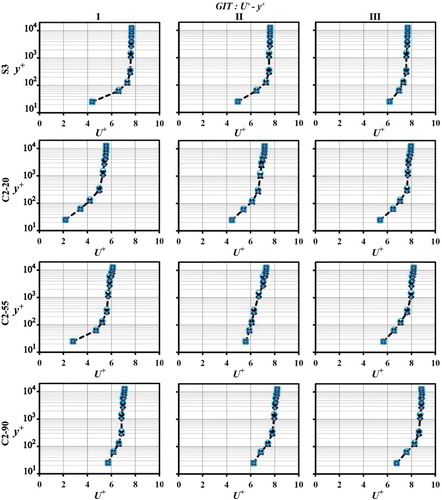
Figure 6. Grid independency test for TKE over four cross-sections and three columns; -x- values corresponding to the standard grid (O), • 20% finer grid (O+ 20), O 20% coarser grid (O-20).

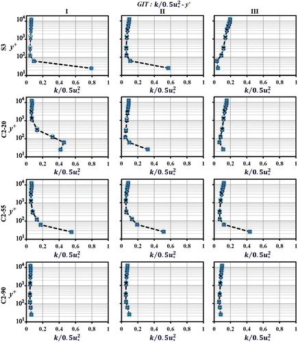
The standard, refined and coarser grids show very similar results. As for velocity profiles (Figure 5), the column near to the centerline of the flume (II) shows the best similarity for all observed cross-sections. Nevertheless, the other profiles also exhibit good similarity of results for both grids. The small differences in the results stem from the empirical equations used to resolve boundary layers. The comparison of TKE results also confirms the adequate quality of the standard grid (Figure 6). Based on the discussed GIT and because the standard grid returns valid results using an optimum amount of computational resources, it was selected for all subsequent simulations.

5.2. Comparison of turbulence models for a racetrack flume

Based on the racetrack flume experiment, three turbulence models were compared using the RSim-3D solver: the standard model, the classical and the improved , as described in Section 2 for three different Froude numbers. The results are provided for four cross-sections and three measurement columns (the same positions as for the GIT profiles: see Figure 1c). The Froude number is a dimensionless variable applied in fluid dynamics studies where the weight of fluid is a predominant force. Generally, this is the case for fluids with a free surface (i.e. rivers, irrigation and drainage open channels). The Froude number is a key hydraulic property in fluvial studies and has a major role in classifying the nature of the flow (i.e. state of the flow condition); therefore, three independent simulations were conducted to cover a broader scope of characteristics based on Froude number alterations.

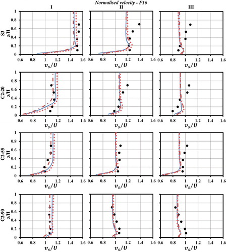
The simulated and measured streamwise mean velocity profiles for F-5 demonstrate a good agreement (Figure 7). In S3 (II & III) and C2-20 (II & III), the simulated velocity profiles exhibit a slight deviation compared with the experiments. The observed differences between the measured and the simulated velocity profiles (max. 0.15 ), especially for the measured velocity near the surface, originated from the surface waves induced by the belt-drive. It is not possible to separate the periodical and non-uniform effect of the surface waves from mean averaged velocities; therefore, such slight deviations are expected. As for higher Froude number runs, i.e. F8 and F16 (Figures 8 and 9), the surface velocities diverge from the experimental results; it is a trend from S3 to C2-20. Regardless of slight deviations, the simulated mean velocity is generally restricted to a narrow band of variations (max. width: 0.078 ). This demonstrates an acceptable consistency for all turbulence models. The similarity is particularly verifiable in the centerline columns (II). Near the outer bank, especially in the flume’s curved path (cs. C2-20, C2-55, C2-90), the classical k-ω model shows slightly lower velocity values, whereas the other models demonstrate a higher similarity. Froude number alterations do not affect the trends of the mean velocity profiles.

Figure 7. Streamwise mean velocity profiles for cross-sections S3, C2-20, C2-55 and C2-90 and three columns (I, II, III): — standard ; –•– classical ; … improved ; and • experimental measurements (F5). The experimental points contain approximately 1% uncertainty.

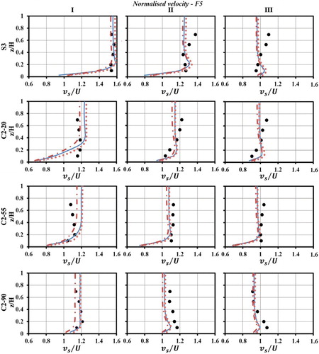
Figure 8. Streamwise mean velocity profiles for cross-sections S3, C2-20, C2-55 and C2-90 and three columns (I, II, III): — standard ; –•– classical ; … improved ; and • experimental measurements (F8). The experimental points contain approximately 1% uncertainty.

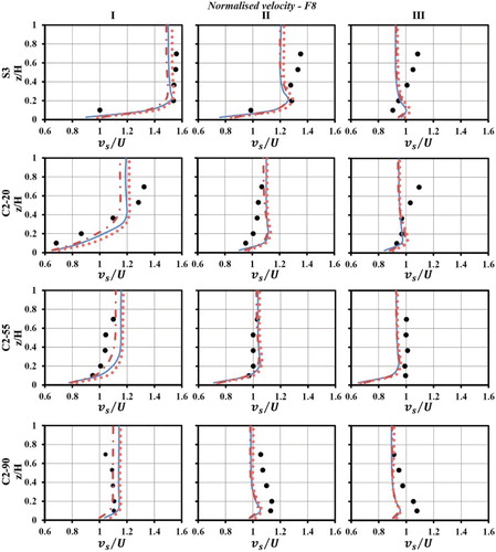
Figure 9. Streamwise mean velocity profiles for cross-sections S3, C2-20, C2-55 and C2-90 and three columns (I, II, III): — standard ; –•– classical ; … improved ; and • experimental measurements (F16). The experimental points contain approximately 1% uncertainty.

Similar to the velocity, the simulated TKE values (Figures 10–12) share a narrow band of variation (max. width: 0.11 ). The standard as well as the classical model, in comparison to the improved runs, yield higher simulated TKE values. The magnitude of differences for the simulated values increases from the outer bank columns (I) toward the inner bank columns (III). The differences are particularly visible in column III. The TKE measurements and simulations show a partial agreement, mostly near the flume’s bed, but an overall discrepancy is evident. One can distinguish two types of differences between measured and simulated TKE profiles: (1) local differences which are visible only in some investigated columns; in this case, simulated and measured profiles show different patterns (e.g. Figure 7: C2-55-I and C2-90-I); (2) differences in the order of magnitude of the turbulence which are observed in all of the investigated columns. In the latter type of differences, distributions of the measured and simulated profiles follow the same pattern, but the measured profiles show higher magnitudes of the TKE.

Figure 10. Turbulent kinetic energy profiles for cross-sections S3, C2-20, C2-55 and C2-90 and three columns (I, II, III): — standard ; –•– classical ; … improved ; and • experimental measurements, the uncertainty band is shown by error bars (F5).

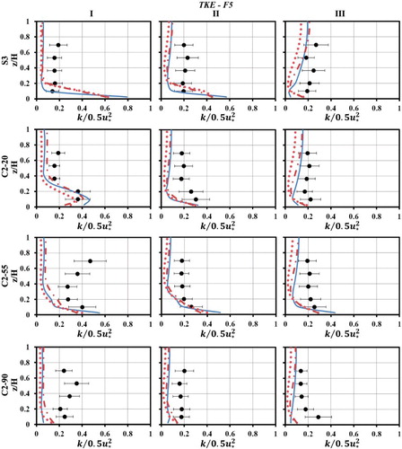
Figure 11. Turbulent kinetic energy profiles for cross-sections S3, C2-20, C2-55 and C2-90 and three columns (I, II, III): — standard ; –•– classical ; … improved ; and • experimental measurements, the uncertainty band is shown by error bars (F8).

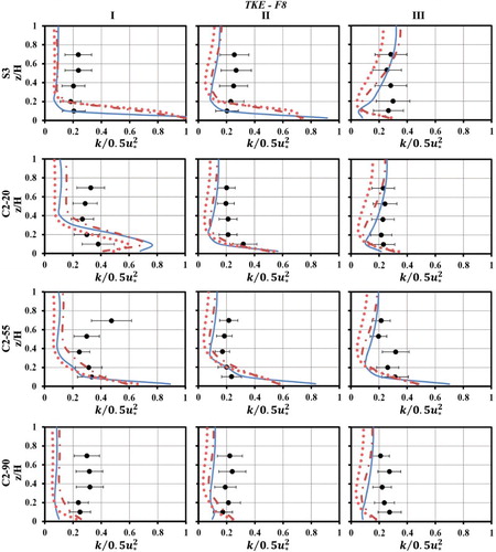
Figure 12. Turbulent kinetic energy profiles for cross-sections S3, C2-20, C2-55 and C2-90 and three columns (I, II, III): — standard ; –•– classical ; … improved ; and • experimental measurements, the uncertainty band is shown by error bars (F16).

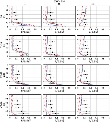
Regarding the first type of differences, turbulence structures in curved channels are known to be affected by the cross-stream motion, streamwise and transversal pressure gradients and curved streamlines. Turbulence models that use a transport equation for each of the Reynolds stresses can resolve these processes. Obviously, such a model is much more computationally expensive; therefore, as an engineering tool, the low-order turbulence closures are widely used for large-scale fluvial simulations. Using these models can cause shortcomings concerning the simulation of local processes. In order to explain the observed differences in the outer bank column (I) of the curved cross-sections (C2-55 and C2-90), one should consider the formation of shear layers along banks of curved channels. The shear layers are characterized by high TKE values (Kang & Sotiropoulos, 2012) and are prone to initiate hydrodynamic instabilities (e.g. outer bank three-dimensional vortices).

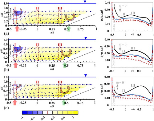
Figure 13 compares the measured depth-averaged values of the normalized turbulent kinetic energy and three numerical variants – as well as vectors of the measured normalized cross-stream velocity components in C2-55 and the contour levels of streamwise component of the vorticity vector – for three different Froude number runs. Streamwise vorticity is calculated from (12) The result is a high TKE zone near the outer bank and exactly at column (I). This shows that a strong shear layer is generated near the outer bank, where the measured TKE profiles demonstrate increased activity. In addition, Figure 13 depicts the formation of two cells of secondary flow in this cross-section; one is the main cell of secondary flow and the other is the outer bank cell, which was observed in almost all of the reported high-resolution measurements of curved channels (Blanckaert & De Vriend, 2005; De Vriend, 1981; Dietrich & Smith, 1983; Farhadi et al., 2017; Kang & Sotiropoulos, 2012). The outer bank cell was observed in (and is expected to extend toward the surface); the mentioned range is the exact range of increased activity in Figures 10–12 (C2-55-I). Also, for higher Froude numbers where the main cell of secondary flow (Figure 13c: right) is stronger, the divergence of measured and simulated results of TKE is higher. Based on the observations, the values of measured and simulated TKE demonstrate better convergence in the proximity of the vorticity zero line () where the flow is characterized by lower three-dimensionality, i.e. weaker secondary flows. Most low-order turbulence models cannot simulate such sophisticated three-dimensional turbulence-induced processes (cf. Koken, Constantinescu, & Blanckaert, 2013). In most large-scale applications (e.g. river restoration and engineering studies), the determination of such flow particularities is not necessary. Therefore, as far as fluvial engineering applications are concerned, the simulation of local, computationally expensive processes is not generally a matter of interest.

Figure 13. Left: vectors of the normalized velocity components in the cross-stream section and contours of the normalized vorticity H/U in C2-55. The red and green arrows indicate the approximate locations of the outer bank and main cell of secondary flow ‘circulation centers’, respectively. Circular arrows show sense of motion for the main secondary flow (counter-clockwise) and outer bank cell (clockwise). The simulation columns I, II and III are indicated for (a) F5, (b) F8 and (c) F16. Right: depth-averaged values of normalized turbulent kinetic energy for cross-section C2-55 for corresponding runs: — standard ; –•– classical ; … improved ; and — experimental measurements.

The second type of difference mentioned above involves the underestimation of the order of magnitude of turbulence by numerical models. The structure of turbulence in open channels is sensitive to the streamline curvature (Farhadi, Sindelar, Tritthart, Glas, & Habersack, 2016). The turbulence in bends is an order of magnitude larger than that in straight reaches (Blanckaert & De Vriend, 2005). Accordingly, most of the RANS solvers for large-scale engineering applications, including RSim-3D, and their implemented turbulence models, were parameterized using straight (i.e. non-curved) flows. Unmodified low-order models require empirical curvature corrections to achieve the same level of agreement with the measurement (Cheng & Farokhi, 1992; Gibson & Rodi, 1981). In the racetrack study, the entire flow domain is affected by the flume’s geometry (i.e. semi-circular plan) and consequently by curved streamlines; this effect cannot be ignored, even for the short straight reach between two bends. Therefore, based on the current settings, the observed differences in turbulence magnitudes are inevitable. The observed complexities of TKE simulations for strong curvilinear flows calls for cautiously using the results to investigate turbulence-related processes (e.g. hydraulic erosions, turbulent sediment transport, etc.). It would also be desirable to modify the model in the case of strong curvilinear flows. In addition, the effect of the belt-drive motion on the measured TKE profiles has to be considered. Parasitical noise (here originating from the belt-drive system) is uniformly distributed over the investigated frequency and does not affect the time-averaged velocities, although it has a negative effect on turbulence investigations (Blanckaert & Lemmin, 2006). It is noteworthy to mention that the simulations exhibit an offset to the measurements which can be described by a normalization multiplier that takes a constant value of 0.445 for all TKE profiles. This constant can be used to downscale the measured profiles to the simulation spectra in the current study. Since the effect is constant over all measurement runs, one can consider this as the belt-drive effect on the measured TKE profiles.

5.3. Comparison of turbulence models for a natural river reach

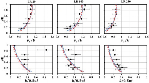
In addition to the laboratory experiments, the second part of the experimental study (Tritthart et al., 2014), i.e. Witzelsdorf field measurements, was designed to compare the three variants of turbulence models. A polyhedral unstructured mesh of 25,287 computational points with a hexagonal base and 7 vertical layers (Figure 14) was used to simulate mean flow and turbulence along 3 kilometers of the river reach. The grid’s maximum skewness and average aspect ratio are 0.56 and 1.93, respectively. Since the simulated reach was previously modeled for the same boundary conditions using different grids and for different objectives (see Tritthart et al., 2014 and Lechner et al., 2014), the solutions are grid independent. Regarding the ‘measurement grid’ in cross-section 1892.3 (Figure 2), three out of eight measurement columns were chosen to correspond to the racetrack flume comparison columns (i.e. I, II and III). Accordingly, columns LR50, LR140 and LR230 were selected for further investigations.

Figure 14. Top view of Witzelsdorf’s simulation mesh.

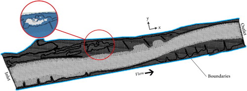
Figure 15 compares velocity and TKE measurements to the simulation results. As was confirmed in the racetrack flume, the three turbulence models – with only negligible divergence – also simulate velocity profiles in a very good agreement with the field measurements in Witzelsdorf. Regarding TKE simulations, model and experimental studies show considerable differences based on the field investigations. A partial agreement between model and measurements is perceptible near the channel’s bed. This observation is also in line with the racetrack flume experiment. Based on the established scientific knowledge in fluvial hydraulics, almost every natural stream features strong three-dimensionalities of flow. In the case of the Witzelsdorf measurements the straight reach is heavily influenced by secondary flows of the second kind (i.e. turbulence-induced secondary flows) which are typical for straight channel reaches. The three-dimensionality is increased by the effect of groynes. Therefore, as observed in the racetrack experiment, the presence of turbulence-induced secondary flow hinders the model from delivering a precise TKE simulation. None of the three compared turbulence models shows a significant improvement.

Figure 15. Streamwise mean velocity (top) and turbulent kinetic energy profiles (bottom) for cross-sections 1892.3, columns LR50, LR140 and LR230: — standard ; –•– classical ; … improved ; and • experimental measurements of Witzelsdorf field investigations, the uncertainty band is shown by error bars.

5.4. Computational expenses

Engineering problems often face time limitations and increasingly require fast and reliable solutions. Therefore, an important task in engineering simulations is to reduce the computational expenses. Table 3 presents the parameters indicating computational performance: CPU time until convergence and the corresponding number of iterations. The convergence criteria were set forth as solution residuals of less than 0.005. RSim-3D uses a Gauss-Seidel solver to compute the solution of the system of linear equations for all of the investigated turbulence models. The simulations were intentionally conducted on one distinct machine of a computational cluster. Their CPU time can therefore be considered as a characteristic parameter to compare the execution time of different turbulence models. Considering the ‘iterations per minute’ parameter, the standard and the classical models share a similar numerical behavior. This yields a matching computational speed. In contrast, the improved model provides a slightly increased computational speed. For all racetrack runs (i.e. F5, F8 and F16), turbulence models exhibit the same characteristics. As for the natural stream simulation, based on the Witzelsdorf field studies (WTZ), the large-scale simulation also shows similar characteristics of computational expenses.

Table 3. Computational expenses of the different turbulence models.

Case	Turbulence model	CPU time until convergence	Total number of iterations	Iterations per minute
F-5	Standard	7h22’57”	8217	18.55
	Classical	7h22’59”	8258	18.64
	Improved	7h54’50”	9009	18.97
F-8	Standard	10h35’26”	9893	15.57
	Classical	10h35’03”	9811	15.44
	Improved	12h50’36”	14210	15.70
F-16	Standard	15h02’12”	12305	13.64
	Classical	15h17’37”	12190	13.28
	Improved	17h09’23”	14703	14.28
WTZ^a	Standard	23h40’57”	16516	11.63
	Classical	23h37’07”	16015	11.30
	Improved	57h22’57”	39949	11.66

^aDanube’s reach simulation south of Witzelsdorf.

6. Conclusions

Racetrack flumes are often used in experimental and numerical studies in ecohydraulics and sediment research. Here, we use conventional turbulence models to investigate the limitations of such applications. Within this framework, three different turbulence models were compared to the experimental data. Simulations were performed using a RANS solver (i.e. RSim-3D). Previously, the standard model had been applied extensively with the solver and verified using different experimental results. Here, we add two different turbulence models (i.e. the classic and an improved version of the model) to RSim-3D to examine the possible differences between these models and their corresponding shortcomings. The mean velocity results using three turbulence models are consistent and evolve within a narrow band of results. This demonstrates agreement with the experimental data, despite some limited discrepancy in patterns. These minor differences among the results of the three models, and the insignificant differences regarding the Froude number changes (i.e. Fr = 0.05 ∼ 0.16), makes it feasible to apply any of the investigated models to simulate the mean flow field, even in the case of strong secondary flows. Our study thus confirms the application of the model to common simulation tasks such as habitat modeling, which is sensitive to the mean flow velocity field. Nonetheless, regarding the comparison of TKE profiles, the simulated and measured profiles exhibit rather weak correlations. This observation, which is confirmed by different Froude ranges of flow in both the racetrack flume and field investigations, dismisses the application of the studied models for ‘turbulence sensitive’ processes. The different turbulence models do not considerably influence TKE profiles. Note that in the current study the applied k-ω models are limited by wall functions which hinder them from achieving their full predictive capability. Nevertheless, one should consider that very fine boundary resolutions for large-scale fluvial simulations – if not infeasible, as confirmed by computational expenses – are unachievable based on the current common state of computational power. A concern regarding the numerical simulations is a sufficient number of cells covering vertically the height of the domain. In large-scale fluvial simulations a minimum number of vertical layers required to cover the three-dimensionality of the flow is reported in literature, e.g. five (Fischer-Antze, Olsen, & Gutknecht, 2008; Fischer-Antze, Rüther, Olsen, & Gutknecht, 2009) to eight layers as reported by Tritthart et al. (2011). However, when the model is applied to smaller scales, due to the lack of proper near-wall treatment algorithms and refinement, the results tend to diverge from the measured values. This effect is more pronounced in turbulence simulations. Adding respective algorithms to the model has the potential to solve issues of turbulence imprecision, though at the same time reducing the code’s applicability for large-scale simulations due to substantial performance decrease in terms of the computational time required.

Two general conclusions can be drawn from our results. First, turbulent structures such as outer and inner boundary vortices, as well as secondary currents of the second kind which are encountered in straight open channels, i.e. turbulence-induced vorticities, cannot be resolved using any of the investigated low-order turbulence models. In such cases, the user should decide whether the local turbulent structures indeed contain crucial information for the task at hand or whether they can be neglected in view of the general context. Most large-scale river engineering applications do not require resolving the details of turbulent structures. The second conclusion pertains to the order of magnitude of turbulence. Here, the effect of the curvilinear flow (secondary flow of the first kind) is simulated without modifying the basic closure hypothesis; therefore, the magnitude of turbulence is underestimated. This calls for exercising caution in using the typical RANS turbulence model results on the TKE and turbulence-related processes in fluvial studies when the flow is dominated by secondary currents.

Disclosure statement

No potential conflict of interest was reported by the authors.

References

- Abad, J. D., & Garcìa, M. H. (2009). Experiments in a high amplitude Kinoshita meandering channel: 1. Implications of bend orientation on mean and turbulent flow structure. Water Resources Research, 45(2), doi: 1029/2008WR007016
- Asnaashari, A., Akhtari, A. A., Dehghani, A. A., & Bonakdari, H. (2016). Experimental and numerical investigation of the flow field in the gradual transition of rectangular to trapezoidal open channels. Engineering Applications of Computational Fluid Mechanics, 10(1), 272–282. doi: 10.1080/19942060.2016.1149102
- Beaulieu, S. E., Sengco, M. R., & Anderson, D. M. (2005). Using clay to control harmful algal blooms: Deposition and resuspension of clay/algal flocs. Harmful Algae, 4(1), 123–138. doi: 10.1016/j.hal.2003.12.008
- Blanckaert, K., & De Vriend, H. J. (2005). Turbulence characteristics in sharp open-channel bends. Physics of Fluids, 17(5), 055102. doi: 10.1063/1.1886726
- Blanckaert, K., & Lemmin, U. (2006). Means of noise reduction in acoustic turbulence measurements. Journal of Hydraulic Research, 44(1), 3–17. doi: 10.1080/00221686.2006.9521657
- Cheng, G. C., & Farokhi, S. (1992). On turbulent flows dominated by curvature effects. Journal of Fluids Engineering, 114(1), 52–57. doi: 10.1115/1.2909999
- De Vriend, H. (1981). Steady flow in shallow channel bend (Doctoral dissertation). Delft University of Technology.
- Dietrich, W. E., & Smith, J. D. (1983). Influence of the point bar on flow through curved channels. Water Resources Research, 19(5), 1173–1192. doi: 10.1029/WR019i005p01173
- Farhadi, A., Sindelar, C., Tritthart, M., Glas, M., Blanckaert, K. & Habersack, H. (2017). An investigation on the outer bank cell of secondary flow in channel bends. Journal of Hydro-Environment Research. doi: 10.1016/j.jher.2017.10.004
- Farhadi, A., Sindelar, C., Tritthart, M., Glas, M., & Habersack, H. (2016). An experiment on turbulent intensities and their contribution to the turbulent kinetic energy in the open channel bend. Proceedings of the International Conference on Fluvial Hydraulics, River Flow 2016, IAHR, St. Louis.
- Farhadi, A., Tritthart, M., Glas, M., & Habersack, H. (2014). Experiments on two consecutive open channel bends. Proceedings of the International Conference on Fluvial Hydraulics, River Flow 2014, IAHR, Lausanne.
- Ferziger, J. H., & Péric, M. (2002). Computational methods for fluid dynamics. Heidelberg: Springer.
- Fischer-Antze, T., Olsen, N. R. B., & Gutknecht, D. (2008). Three-dimensional CFD modelling of morphological bed changes in the Danube river. Water Resources Research, 44(9), 327 W09422. doi: 10.1029/2007WR006402
- Fischer-Antze, T., Rüther, N., Olsen, N. R. B., & Gutknecht, D. (2009). Three-dimensional (3D) modeling of non-uniform sediment transport in a channel bend with unsteady flow. Journal of Hydraulic Research, 47(5), 670–675. doi: 10.3826/jhr.2009.3252
- Fu, C., Uddin, M., & Curley, A. (2016). Insights derived from CFD studies on the evolution of planar wall jets. Engineering Applications of Computational Fluid Mechanics, 10(1), 44–56. doi: 10.1080/19942060.2015.1082505
- Fuhrman, D. R., Dixen, M., & Jacobsen, N. G. (2010). Physically-consistent wall boundary conditions for the k-ω turbulence model. Journal of Hydraulic Research, 48(6), 793–800. doi: 10.1080/00221686.2010.531100
- Gibson, M. M., & Rodi, W. (1981). A Reynolds-stress closure model of turbulence applied to the calculation of a highly curved mixing layer. Journal of Fluid Mechanics, 103, 161–182. doi: 10.1017/S0022112081001286
- Goldberg, U. C., & Batten, P. (2015). A wall-distance-free version of the SST turbulence model. Engineering Applications of Computational Fluid Mechanics, 9(1), 33–40. doi: 10.1080/19942060.2015.1004791
- Harii, S., & Kayanne, H. (2002). Larval settlement of corals in flowing water using a racetrack flume. Marine Technology Society Journal, 36(1), 76–79. doi: 10.4031/002533202787914188
- Hauer, C., Unfer, G., Tritthart, M., Formann, E., & Habersack, H. (2011). Variability of mesohabitat characteristics in riffle-pool reaches: Testing an integrative evaluation concept (FGC) for MEM-application. River Research and Applications, 27(4), 403–430. doi: 10.1002/rra.1357
- Hellsten, A. K. (2005). New advanced kw turbulence model for high-lift aerodynamics. AIAA Journal, 43(9), 1857–1869. doi: 10.2514/1.13754
- Kang, S., & Sotiropoulos, F. (2012). Assessing the predictive capabilities of isotropic, eddy viscosity Reynolds-averaged turbulence models in a natural-like meandering channel. Water Resources Research, 48(6), 353 W06505:1-12. doi: 10.1029/2011WR011375
- Khosronejad, A., Rennie, C. D., Salehi Neyshabouri, S. A. A., & Townsend, R. D. (2007). 3D numerical modeling of flow and sediment transport in laboratory channel bends. Journal of Hydraulic Engineering, 133(10), 1123–1134. doi: 10.1061/(ASCE)0733-9429(2007)133:10(1123)
- Kok, J. C. (2000). Resolving the dependence on freestream values for the k-turbulence model. AIAA Journal, 38(7), 1292–1295. doi: 10.2514/2.110
- Koken, M., Constantinescu, G., & Blanckaert, K. (2013). Hydrodynamic processes, sediment erosion mechanisms, and Reynolds number induced scale effects in an open channel bend of strong curvature with flat bathymetry. Journal of Geophysical Research: Earth Surface, 118(4), 2308–2324. doi: 10.1002/2013JF002760
- Larsen, L. G., Harvey, J. W., & Crimaldi, J. P. (2009). Morphologic and transport properties of natural organic floc. Water Resources Research, 45(1), 339. doi: 10.1029/2008WR006990
- Launder, B. E., & Spalding, D. B. (1974). The numerical computation of turbulent flows. Computer Methods in Applied Mechanics and Engineering, 3(2), 269–289. doi: 10.1016/0045-7825(74)90029-2
- Lechner, A., Keckeis, H., Schludermann, E., Loisl, F., Humphries, P., Glas, M., … Habersack, H. (2014). Shoreline configurations affect dispersal patterns of fish larvae in a large river. ICES Journal of Marine Science, 71(4), 930–942. doi: 10.1093/icesjms/fst139
- Liedermann, M., Tritthart, M., & Habersack, H. (2013). Particle path characteristics at the large gravel-bed river Danube: Results from a tracer study and numerical modelling. Earth Surface Processes and Landforms, 38(5), 512–522. doi: 10.1002/esp.3338
- Menter, F., Ferreira, J. C., Esch, T., & Konno, B. (2003). The SST turbulence model with improved wall treatment for heat transfer predictions in gas turbines. In Proceedings of the International Gas Turbine Congress, Tokyo, IGTC2003-TS-059.
- Menter, F. R. (1994). Two-equation eddy-viscosity turbulence models for engineering applications. AIAA Journal, 32(8), 1598–1605. doi: 10.2514/3.12149
- Nezu, I., & Nakagawa, H. (1993). Turbulence in open channels. Rotterdam: AA Balkema.
- Nieto, F., Hargreaves, D. M., Owen, J. S., & Hernández, S. (2015). On the applicability of 2D URANS and SST k-ω turbulence model to the fluid-structure interaction of rectangular cylinders. Engineering Applications of Computational Fluid Mechanics, 9(1), 157–173. doi: 10.1080/19942060.2015.1004817
- Nowell, A. R., Jumars, P. A., Self, R. F., & Southard, J. B. (1989). The effects of sediment transport and deposition on infauna: Results obtained in a specially designed flume. In Ecology of marine deposit feeders (pp. 247–268). New York, NY: Springer.
- Peralta, C., Parente, A., Balogh, M., & Benocci, C. (2014). RANS simulation of the atmospheric boundary layer over complex terrain with a consistent k-epsilon model formulation. Proceedings of the 6th International Symposium on Computational Wind Engineering (CWE2014), 236–237.
- Roache, P. J. (1998). Verification of codes and calculations. AIAA Journal, 36(5), 696–702. doi: 10.2514/2.457
- Rudra Reddy, K., & Durbin, P. (2013). Formulation of a k-omega based DDES model. APS Division of Fluid Dynamics Meeting Abstracts, 4009.
- Schieber, J. (2016). Experimental testing of the transport-durability of shale lithics and its implications for interpreting the rock record. Sedimentary Geology, 331, 162–169. doi: 10.1016/j.envpol.2016.07.055
- Schieber, J., Southard, J., & Thaisen, K. (2007). Accretion of mudstone beds from migrating floccule ripples. Science, 318(5857), 1760–1763. doi: 10.1126/science.1147001
- Schludermann, E., Tritthart, M., Humphries, P., & Keckeis, H. (2012). Dispersal and retention of larval fish in a potential nursery habitat of a large temperate river: An experimental study. Canadian Journal of Fisheries and Aquatic Sciences, 69(8), 1302–1315. doi: 10.1139/f2012-061
- Tritthart, M. (2005). Three-dimensional numerical modelling of turbulent river flow using polyhedral finite volumes (Doctoral dissertation). Vienna University of Technology, Vienna.
- Tritthart, M., Glas, M., Liedermann, M., & Habersack, H. (2014). Numerical Study of Morphodynamics and Ecological Parameters Following Alternative Groyne Layouts at the Danube River. Proceedings of 11th International Conference on Hydroscience & Engineering, Hamburg, 684–692.
- Tritthart, M., & Gutknecht, D. (2007). Three-dimensional simulation of free-surface flows using polyhedral finite volumes. Engineering Applications of Computational Fluid Mechanics, 1(1), 1–14. doi: 10.1080/19942060.2007.11015177
- Tritthart, M., Liedermann, M., & Habersack, H. (2009). Modelling spatio-temporal flow characteristics in groyne fields. River Research and Applications, 25(1), 62–81. doi: 10.1002/rra.1169
- Tritthart, M., Mayrhofer, A., Glas, M., Glock, K., & Habersack, H. (2015). Comparison of the k-epsilon and k-omega turbulence models in a laboratory and a river modeling context. E-proceedings of the 36th IAHR World Congress, The Hague.
- Tritthart, M., Schober, B., & Habersack, H. (2011). Non-uniformity and layering in sediment transport modelling 1: Flume simulations. Journal of Hydraulic Research, 49, 325–334. doi: 10.1080/00221686.2011.583528
- Tritton, D. J. (1977). Physical fluid dynamics. New York, NY: Van Nostrand Reinhold. doi: 10.1007/978-94-009-9992-3
- Versteeg, H. K., & Malalasekera, W. (2007). An introduction to computational fluid dynamics: The finite volume method. New York, NY: Pearson Education.
- Wang, P., Hu, B., Wang, C., & Lei, Y. (2015). Phosphorus adsorption and sedimentation by suspended sediments from Zhushan Bay, Taihu lake. Environmental Science and Pollution Research, 22(9), 6559–6569. doi: 10.1007/s11356-015-4114-6
- Wilcox, D. C. (1988). Reassessment of the scale-determining equation for advanced turbulence models. AIAA Journal, 26(11), 1299–1310. doi: 10.2514/3.1004
- Wilcox, D. C. (2008). Formulation of the k-ω turbulence model revisited. AIAA Journal, 46(11), 2823–2838. doi: 10.2514/1.36541