Development and testing of a soot particle concentration estimator using Lagrangian post-processing

ABSTRACT

Soot emissions from combustion devices are known to have harmful effects on the environment and human health. As the transportation industry continues to expand, the development of techniques to reduce soot emissions remains a significant goal of researchers and industry. In order for current soot modeling techniques to be reliably accurate, they must incur an intractably high computational cost. This project leverages existing knowledge in soot modeling and soot formation fundamentals to develop a stand-alone, computationally inexpensive soot concentration estimator to be linked to Computational Fluid Dynamics simulations as a post-processor. Preliminary development and testing of the estimator is presented here for laminar flames. As soot properties cannot be determined by local conditions, the estimator consists of a library generated using the hystereses of soot-containing fluid parcels, which relates soot concentration to the aggregated gas-phase environment histories to which a fluid parcel has been exposed. The estimator can be used to relate soot concentration to computed parcel hystereses through interpolation techniques. The estimator shows the potential ability to produce accurate results with very low computational cost in laminar coflow diffusion flames. Results also show that as flame data representing a broader set of conditions (temperature, mixture fraction, residence time, etc.) are added to the library, the estimator becomes applicable to a wider range of flames.

KEYWORDS:

• Soot concentration
• soot emissions
• estimator
• Lagrangian parcel-tracking

1. Introduction

Black carbon particulate (soot) is generated in a variety of combustion systems. Combustion processes have a key role in burners, power production devices, and the transportation industry. The emission of combustion-generated soot is a serious threat to human health and a growing concern. Populations living in dense urban areas show higher rates of lung and heart diseases because of high concentrations of pollutants that contain compounds such as nitrogen oxides, carbon monoxide, and soot particles in the atmosphere (Beniwal & Shivgotra, 2009; Shiraiwa, Selzle, & Poschl, 2012). Furthermore, both small and large soot particles can cause significant environmental problems. Small soot particles in the atmosphere absorb sunlight and warm the surrounding air, while larger and darker particles that fall to the ground accelerate the melting of snow and ice, since dark particles absorb sunlight (Daly, 2012). These effects contribute to global climate change. As a consequence, stricter soot emission regulations are being imposed while others are expected in the near future (EPA sets stricter clean air standard for soot, 2015). Industries and combustion device designers are being required to reduce soot particles emitted from combustion. Therefore, searching for and developing techniques to reduce soot formation and emissions has become an important concern for researchers and industry.

In the design of industrial combustion devices, such as engines, detailed numerical modeling and Computational Fluid Dynamics (CFD) simulations have become commonplace. Current capabilities allow for simulation of the chemical reactions, ignition, and burning of fuels in turbulent flow inside realistic engine geometry at high, but tractable computational cost. Data from these simulations aid in the engine design, construction, and improvement processes. However, the inclusion of soot formation within these simulations is challenging, and if it is to be reliably accurate, it incurs an intractably high computational cost. Thus, it is a major objective of the combustion industry to develop novel numerical techniques to model, predict, or estimate soot concentrations. The objective of this work is to develop a soot concentration estimator to be used as a post-processor of CFD data, to aid combustion device designers in reducing emissions. The present work does not propose a model for soot formation and oxidation, rather it seeks to develop a system of library generation that can be used to estimate soot properties using correlations and interpolation.

Soot formation is considered to be an extremely complex phenomenon that includes chemical kinetics, thermodynamics, particle dynamics, heat transfer, and multiphase flow. In order to understand this complexity, it is necessary to consider the progress of numerical modeling of combustion and soot formation that has been made previously. Early techniques used in the literature to model soot include the two-equation formulation (Liu, Guo, Smallwood, & Gulder, 2003; Said, Garo, & Borghi, 1997), the method of moments (MOM) (Frenklach & Wang, 1991; Zhong, Dang, Song, & Gong, 2012), stochastic method (Brownh & Heywood, 1988; Celnik, Sander, Raj, West, & Kraft, 2009). As the understanding of soot formation and computational power have improved over the years, so has the complexity of soot models. Many of the works studied have implemented the sectional method to model soot formation and kinetics (Chernov, Thomson, Dworkin, Slavinskaya, & Riedel, 2014; Chernov, Zhang, Thomson, & Dworkin, 2012; Dworkin, Cooke, et al., 2009; Dworkin, Smooke, & Giovangigli, 2009; Dworkin, Zhang, Thomson, Slavinskaya, & Riedel, 2011; Park, Rogak, Bushe, Wen, & Thomson, 2005; Sirignano, Kent, & D’Anna, 2015; Smooke, McEnally, Pfefferle, Hall, & Colket, 1999; Smooke, Long, Connelly, Colket, & Hall, 2005; Wen, Thomson, Lightstone, Park, & Rogak, 2006). While these works have focused on atmospheric pressure flames, recently studies on modeling soot at elevated pressures have been conducted as well (Eaves, Thomson, & Dworkin, 2013; Hunter, Litzinger, Wang, & Frenklach, 1996).

According to Kennedy (1997), soot models can be divided into three classifications: empirical soot models, semi-empirical soot models, and detailed soot models. Empirical soot models come from experimental phenomenological correlations of soot formation rates with combustion conditions such as pressure and temperature (Harris, King, & Laurendeau, 1986; Olson, Pickens, & Gill, 1985). These kinds of models are easily understandable, easy to implement, and they do not require significant additional computational cost. The low computational cost requirement is the main reason that this kind of modeling is so common in the literature related to gas turbines and diesel engines, as the geometrical complexity of these devices already pushes the limits of modern computational resources. Although the application of the aforementioned models is common, the loss of accuracy and comprehensive understanding into the soot formation processes are its weakness.

Semi-empirical soot models are purported to incorporate physical phenomena, chemical aspects, and also experimental data. Fairweather, Jones, and Lindstedt (1992) proposed a two-equation soot model, which has been used widely. This model neglects the aggregate structure and polydispersity of soot particles; thus, although it can give some insight into soot formation mechanisms, it is not detailed enough to deliver soot properties such as aggregate structure and size distribution. Another weakness of this model type is that it does not involve the resolution of Polycyclic Aromatic Hydrocarbons (PAH) chemistry in a detailed manner. Therefore, researchers cannot use this type of model to study the interactions of aromatic species and soot. Furthermore, these models require the use of empirically tuned parameters, and are not broadly applicable when applied to combustion conditions that differ from those for which the model was developed. These models often fail to predict trends or even order-of-magnitude values for soot concentrations. The estimator presented in this study seeks to address this issue by being developed to be applicable to a wide range of industrial combustion devices.

As knowledge of soot formation processes advanced, the complexity of soot models increased. Various approaches have been developed for detailed modeling of soot formation under simultaneous nucleation, coagulation, oxidation and surface growth processes. Some of the methods in literature that represent these approaches include the abovementioned method of moments, sectional method, and stochastic method. Investigating the mean properties and the size distribution of soot particles can be achieved using a sectional aerosol dynamics model. Park et al. (2005) proposed an advanced sectional model that solves two equations (number densities of both primary particles and aggregates) per section, in order to model the evolution and fractal-like structure of soot. Soot formation in plug flow reactors (Park et al., 2005) and shock tubes (Wen, Thomson, Lightstone, & Rogak, 2006) have been modeled with high accuracy using the aforementioned model. However, it should be noted that the improvement in accuracy of detailed soot models comes at the expense of high computational cost. This is another issue addressed by the estimator presented in this study.

Despite the variation in model types in the literature, there are some common steps of modeling soot formation and oxidation. The first component of an accurate model is the prediction of the flow field by solving the Navier-Stokes equations. Solving the gas-phase chemistry equations, soot-gas chemistry, and soot aerosol dynamics equations is necessary to model soot structure as well as nucleation and surface growth/oxidation reactions (Eaves et al., 2013). Modeling thermal radiation by solving radiative heat transfer is also normally needed for accurate temperature field prediction (Zhang, 2009). In recent years, many researchers have used these steps in order to model soot formation and oxidation (Chernov et al., 2012, 2014; Dworkin, Cooke, et al., 2009; Dworkin, Smooke, et al., 2009; Dworkin et al., 2011; Eaves et al., 2013; Sirignano et al., 2015; Smooke et al., 1999, 2005; Wen, Thomson, Lightstone, Park, et al., 2006; Zhao et al., 2003).

In designing industrial combustion devices where turbulent combustion is prevalent, detailed CFD simulations are typically utilized. Commonly used models include the flamelet approach (Peters, 1984) and inter-layer diffusion model (Jaberi & Givi, 1995). These models are capable of simulating chemical reactions, the burning of fuels, ignition and other flow/combustion processes in a real engine. Furthermore, Large Eddy Simulations (LES) and Direct Numerical Simulations (DNS) are utilized to accurately model the performance of gas turbines and engines. Combustion device designers can use the data from simulations to evaluate potential design modifications and make product performance more efficient. However, studying and simulating soot formation in turbulent combustion using these techniques has high computational cost, and is considered to be quite challenging (Adedoyin, Walters, & Bhushan, 2015; Attili, Bisetti, Mueller, & Pitsch, 2016; Koo, Hassanaly, Raman, Mueller, & Geigle, 2016; Su, Li, Li, Wei, & Zhao, 2012; Tang, Guo, & Ranjan, 2015). As a result, soot formation is neglected in most industrial device simulations, which emphasizes the need for a low computational cost CFD post-processor for predicting soot emissions.

Studies on soot formation processes are mostly focused on investigating the relationship between hydrocarbon fuels and soot, and how it effects soot production in different combustion process. A preponderance of these studies provides valuable understanding that can be applied to the development of an estimator. For example, the characteristic time of soot formation is long compared to that of combustion kinetics, and thus local conditions cannot be used to correlate soot properties within a library. Instead, fluid parcel histories throughout the entire combustion system need to be considered. Furthermore, the final mass of particles emitted from the system can vary based on the particle after-burning process and oxidation, which depend on the combustion configuration (Glassman, 1989). The current work has leveraged this understanding to develop a computationally efficient stand-alone fluid parcel-tracking post-processor, capable of predicting soot concentrations in industrially-relevant configurations.

The next section of this work will discuss the methodology used in the development of the soot concentration estimator. Section 3 reports results of testing and validation in terms of computational cost and predictive capabilities of the estimator. Lastly, Section 4 will summarize the conclusions of the work.

2. Methodology

Since the main goals of this study are designing and generating a soot concentration estimator that does not rely on additional CFD modeling, choosing the appropriate strategy and methods which provide a tool of low computational cost, ease of use, and high accuracy are the primary objectives. This section describes the general theory and process behind the estimator's development and the associated methodology.

Steady, axisymmetric, laminar coflow diffusion flames, among different combustion configurations (Constantine & Richard, 1989; Dworkin et al., 2011; Eaves et al., 2012; Liu et al., 2003), have a reasonably simple flow field and hence are pertinent to study both numerically and experimentally. Moreover, a platform for studying the evolution of soot aggregates and the relations between soot formation and gas-phase chemistry in multi-dimensional scales can be provided by studying these flames. This kind of flame provides opportunities to investigate both soot formation and oxidation processes by encompassing regions from soot nucleation and also soot oxidation (Khosousi & Dworkin, 2015). Furthermore, three-dimensional measurements of flame and soot quantities can be facilitated since both soot formation and oxidation in these flames cover a wide region (Legros et al., 2006). The aforementioned reasons have motivated researchers to pay attention to this type of flame. Thus, laminar coflow diffusion flames are systems for which there is an abundance of experimental data that can be accurately modeled using CFD; therefore, they present an appropriate initial testing bed for new estimator development.

Referring to Figure 1, the first step in the development of the estimator is to gather validated flame simulation and soot formation data, which can be used to populate the library. The flames used initially in this study are the laminar coflow ethylene diffusion flames studied originally by Santoro, Semerjian, and Dobbins (1983), Smyth and Shaddix (1996), and the diluted ethylene flames studied by Smooke et al. (2005), hereafter known as the Santoro, Smyth, and Smooke flames, respectively. The burner dimensions and flow conditions of the experiments are summarized in Table 1. The numerical values contained in the Smooke flame names represent the ethylene dilution ratio (for example, ‘Smooke32’ refers to the Smooke flame with 32% ethylene in the fuel stream by mole). The numerical values contained in the Smyth flame name represent the fuel velocity in the burner.

Figure 1. Flow chart illustrating development of soot estimator library.

Table 1. Burner dimensions and flow conditions of fuel and air streams for experiments gathered (Santoro et al., 1983; Smooke et al., 2005; Smyth & Shaddix, 1996).

Flame	Inner Diameter (mm)	Outer Diameter (mm)	Air Velocity (cm/s)	Fuel Velocity (cm/s)	Fuel Stream Composition
Santoro	11.1	101.6	13.3	5.06	100% C2H4
Smooke32	4.0	50.0	35.0	35.0	32% C2H4/68% N2
Smooke60	4.0	50.0	35.0	35.0	60% C2H4/40% N2
Smooke82	4.0	50.0	35.0	35.0	82% C2H4/18% N2
Smyth41	11.0	102.0	8.7	4.1	100% C2H4
Smyth46	11.0	102.0	8.7	4.6	100% C2H4
Smyth48	11.0	102.0	8.7	4.8	100% C2H4

The second step in the estimator development is to use the experimental and validated numerical data to build on the existing knowledge of soot formation. As new findings related to soot formation processes are made, they can be implemented into estimator development to improve performance. A careful review of works from Santoro et al. (1983), Smyth and Shaddix (1996), and Smooke et al. (2005) informs the varying nature of soot formation in these flames, and the range of conditions that lead to their differing soot formation characteristics. Step three of estimator development is to generate or retrieve validated CFD data for multiple flames. The purpose of using multiple flames is to broaden the predictive applicability of the estimator for various systems. Coworkers have been using a Eularian CFD approach to predict important local variables such as soot properties, fluid velocities, temperature, and species concentrations in flames (Eaves et al., 2012). The various detailed CFD data sets generated over the past seven years by Dworkin and coworkers (Chernov et al., 2012, 2014; Dworkin et al., 2011; Eaves et al., 2012, 2013; Khosousi & Dworkin, 2015; Veshkini, Dworkin, & Thomson, 2014) are validated against experimental data, and this understanding of soot formation forms the basis of the estimator development. It should be noted that while these studies contain various levels of semi-empirical modeling, the computed soot volume fractions are well validated. Thus, these data sets can be used to relate local soot concentrations to flow hystereses, and are therefore valuable for library generation.

Step four of the estimator development is to determine the library dimensionality and which variable hystereses to use in its generation. From a purely theoretical point of view, the local instantaneous formation and destruction rates of soot particles can be written as a deterministic function of local flow field characteristics as shown in Equation (1). (1) T is the temperature experienced by the soot particle, Y_i is the mole fraction of species i, P is the local pressure of the gas, f_v is soot volume fraction, and A_s is soot surface area at a given moment in time (t). The functional dependence is stronger on some variables (T,  … ) than on others ( … ). The variables considered in this work are soot concentration, mixture fraction, temperature, acetylene concentration, benzene concentration, and O₂ concentration. It should be noted that this list was based in part from a trial-and-error process that has not yet been exhaustive. However, a strong correlation has been shown between mixture fraction and soot concentration (Park, Burns, Buxton, & Clemens, 2017). Also, soot is known to form in flame regions with temperatures between 1300 K and 1600 K (Turns, 2000). O₂ concentration was chosen to capture soot oxidation effects. Lastly, acetylene concentration was chosen because soot formation through surface growth is attributed to acetylene concentration at atmospheric conditions and even more so at elevated pressures (Eaves et al., 2012). Benzene concentration was chosen to represent PAH addition as aromatic rings are commonly observed in PAH structures (Zeng & Chen, 2011). The dependent variable of the library in the present work is soot concentration, however, libraries to predict other soot properties, such as particle sizes could also be developed. The number of independent variables chosen to be included in the soot estimator will determine the library's dimensionality. Also, as knowledge of soot formation advances, more appropriate variables can be included in the library.

Step five of the estimator development uses a Lagrangian parcel-tracking CFD data processor (Veshkini et al., 2014). Theoretically, the formation or destruction of a soot particle is determined by its entire history from inception to oxidation. Therefore, in the present work, it is proposed to integrate variable histories of a fluid parcel in order to generate soot volume fraction correlations. For example, integrated temperature history can be a gauge for relative heat transfer into the particles, which is a suitable indicator of soot processes. The aggregated history of each variable can be expressed by the integral of each local variable with respect to time along a pathline traversed by a fluid parcel that may contain soot. The mathematical definition used herein of integrated temperature, molecular species, and mixture fraction histories are expressed in the following equations: (2) (3) (4)

Where T_h is the integrated temperature history, Y_i,h is the history of species i, and MF_h is the mixture fraction history. In the present work, these integrals will be numerically evaluated by a post-processor considering data from CFD simulations of laminar flames. As a fluid parcel traverses the fluid domain, the histories defined in Equations (2) – (4) continuously increase monotonically.

Corresponding to step five in Figure 1, the Lagrangian parcel-tracking post-processor comprises an algorithm that reads the results of a CFD simulation with a detailed soot model and traces out the path of a soot-containing fluid parcel. The post-processor contains a soot concentration filter that will only begin to track the fluid parcel when the soot concentration value is above the filter value. For the current work, the filter value has been set to 0.1 ppm. This process is depicted graphically in Figure 2, wherein the pathline through the flame is outlined in black in the left side figure and the temperature history is calculated as the area under the curve in the right side figure. As the fluid parcel progresses upward through the flame, the graph on the right side of Figure 2 is traced out. Each progressive point along the fluid parcel pathline corresponds to an increasing time along the x-axis of the right side graph in the figure. To determine the time step from one point to the next, the post-processor divides the domain spacing by the average of the velocity vectors of the corresponding domain nodes. Therefore, the time steps through the pathline of the fluid parcel vary consistently.

Figure 2. Illustration of Lagrangian parcel-tracking post-processor calculating instantaneous temperature along the pathline of a soot-containing fluid parcel. Left side: temperature contours of a laminar ethylene coflow diffusion flame. Right side: Plot of local temperature the soot-containing fluid parcel is exposed to along its pathline.

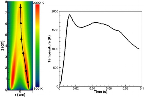
It is important to emphasize here that the estimator does not attempt to relate soot concentration to local conditions, but rather it always considers the ‘accumulated variable history’, and its effect on soot growth or destruction, as characteristic soot times are long compared to chemical times. For example, local temperature does not relate to soot concentration but rather ‘the total history of temperature experienced by the soot-particle containing fluid parcel’ correlates to soot concentration. This post-processor is similar to those that predict NOx emissions (Gobbato, Masi, Toffolo, Lazzaretto, & Tanzinid, 2012; Zhu, Ouyang, & Lu, 2013). The post-processor has been used recently in studies of high pressure flames (Eaves et al., 2013) and particle surface reactivity (Veshkini et al., 2014) for data analysis, and has been repurposed here to extract soot-flow field correlations for library generation.

Step six of the estimator development is to tabulate the histories calculated by the post-processor to generate a library of correlations, as was first done in (Bozorgzadeh, 2012). In the present work, the libraries consist of soot concentration values that are related to MF_h, T_h, and O_2,h. MF_h is chosen to account generally for gas phase conditions that may favor soot growth. For high pressure conditions, acetylene and benzene concentrations are substituted for MF_h, which is discussed later. O₂ is the only oxidative species used in the present library because the focus of the current work is on testing laminar diffusion flames. If a premixed or partially-premixed system were tested, or turbulence were present, evaluating OH_h should be considered.

The range of each variable history, from zero to the maximum value anywhere in the data sets considered, can be divided into a specified number of sections (or bins) in which the midpoints of those bins are used as data entries for the library. When multiple entries exist in a bin (for example from different pathlines in one flame dataset, or from separate data sets), those values are averaged when populating the bin. These data entries constitute the library. As the number of bins utilized increases, the resolution of the library becomes more precise. However, increasing the number of bins used to generate the library will increase the number of data entries in the library significantly due to the multi-dimensionality of the library. Once a library of correlated data has been generated, a test can then be conducted on the predictive capability of the library using validated flame data.

Referring to Figure 3, with a library generated as described above, the utilization of the soot estimator library can be described in three steps. Step one is to compute or otherwise retrieve the CFD data for a combustion system. These CFD data do not need to include soot properties as they will be predicted using the library. They only need to include temperature, a velocity field, and key chemical species concentrations. In theory, the combustion system can be a simple laminar flame or a more complex diesel engine or gas turbine, as long as flow field data are known. Step two consists of computing the hystereses fields of the CFD data using the Lagrangian particle-tracking post-processor described earlier. The hystereses fields are based on the velocity fields throughout the domain of the CFD data. This step can vary greatly in complexity depending on the type of combustion system. For example, for steady laminar flames, the task is trivial, however, for turbulent combustion systems, especially those with swirling flows, the task is more complex and will require greater computational cost. However, it will be more computationally efficient than modeling soot formation in situ. Lastly, step three is to interpolate the hystereses fields in the soot estimator library to determine the soot properties at each point in the domain. The current work focuses on soot concentration, but soot morphology could also be estimated if sufficiently accurate size and shape data were available to generate the library.

Figure 3. Flow chart illustrating utilization of soot estimator library.

3. Testing, validation and discussion

Although the prediction accuracy of the estimator is of primary importance, the computational cost associated with the estimator is an equally important aspect of its development. For practical application and utility, results must be generated in a reasonable amount of time. The majority of computational time required is during library generation. However, it should be noted that one library can be used for multiple soot concentration predictions. A comparison between the time required to generate a library and the number of data entries in that library based on number of bins used, is displayed in Figure 4. It should be noted that for these timings the libraries were generated using only Santoro flame data and the computations were performed on one CPU.

Figure 4. Time required to generate a library and the number of data entries in that library versus the number of bins used.

The 100-bin library required just over one hour of compute time to generate. It can be seen that the time needed to generate a library increases at a greater rate with increasing bin resolution. This behavior is due to the dimensionality of the library causing the number of data entries in the library to grow as the number of bins used increases. By testing the predictive capabilities of the library with varying resolution, a plateau was observed above the 100-bin library above which the change in prediction accuracy did not improve significantly with increasing resolution. The results of this test indicated that a 100-bin library gave a satisfactory compromise between computational cost and predictive capabilities.

Once a library is generated, it can be used for soot concentration predictions of multiple combustion systems. For application purposes, the computational cost incurred on a combustion device designer looking to use this soot estimator as a post-processor to a CFD simulation comes from the Lagrangian parcel-tracker and interpolation of the library. The Lagrangian parcel-tracking post-processor takes under a minute to compute the variable histories from the CFD results for laminar flames on a standard desktop computer. The interpolation of the library to yield a soot prediction requires a few seconds of compute time per pathline. It should be noted that these compute time assessments are associated with simulations of laminar coflow diffusion flames that contain a relatively small amount of elements in the computational domain compared to industrial turbulent simulations. The computational domains of engines and gas turbines can be large and complex. Consequently, the computational cost of the soot estimator is expected to be greater.

It is important to emphasize that the strategy of the estimator is to predict soot concentration, not on local conditions, as it is clear from residence time disparities that local conditions neither determine soot concentrations, nor correlate to them, but rather based on the cumulative soot-particle-containing fluid parcel history. The method used to test the predictive capabilities of the estimator is to compare the estimated values of soot concentration using the library to experimentally validated soot concentrations along two streamlines; the flame centerline and streamline of maximum soot. The first test conducted is an attempt to predict soot concentration in Santoro flame streamlines using a library generated from Santoro and Smooke flame data. Once the library is generated, MF_h, T_h, and O_2,h are calculated along the two streamlines using the Lagrangian particle-tracking post-processor based on validated CFD data used to generate the library. It is important to note that for the tests in the current work, the streamline of maximum soot is known. However, if the soot estimator library is applied to an unknown combustion system, the hystereses fields spanning the combustion domain would need to be calculated to determine the point of maximum soot. These hystereses fields are then interpolated in the four dimensional library to yield a soot concentration estimate based on the correlations in the library, at discrete points along the pathline. The results of the first test are displayed in Figure 5, in which soot concentration is plotted against height above burner.

Figure 5. Comparison of experimentally-validated CFD computed soot concentrations with those predicted by the estimator library for the Santoro et al. (1983) flame along the streamline of maximum soot (left) and the flame centerline (right).

Observing Figure 5, the soot concentration values estimated follow the computed curve very well. One of the main objectives of the proposed estimator is to predict peak soot concentration. The peak soot concentrations for the streamline of maximum soot and flame centerline differ by only 0.3% and 3.1%, respectively. Although the results of Figure 5 are quite promising, there are some sharp deviations in soot concentration estimates that preclude a smooth curve. The non-monotonic behavior of the estimated data is attributable to the nature of the procedure projecting a multi-dimensional library onto a two-dimensional plot. Another reason for this behavior is the averaging of soot concentration values conducted during library generation. As more flame data are added to the library, specific soot concentration values of the original library may be averaged up or down resulting in a non-smooth curve. This effect is more evident in further tests.

It should be noted that the comparison depicted in Figure 5 does not represent a rigorous test of the estimator as Santoro flame soot concentrations were incorporated into the library before then being estimated. Therefore, the applicability of the library is ensured artificially, and these data should be taken with cautious optimism. If this estimator were to be used for predictive purposes, it must be able to predict soot concentration values from flame conditions that may not necessarily be consistent with the flame data used to generate the library. A good strategy is to continually develop and enhance the library (or libraries) using newly available data, so as to broaden its applicability as much as possible. The next step in examining the predictive capabilities of the estimator is attempting to predict soot concentration for streamlines of a flame that is not used in library generation. Therefore, the streamlines of a Smyth48 flame are tested using the library generated from only Santoro and Smooke flame data. The results of the test are displayed in Figure 6.

Figure 6. Comparison of CFD computed soot concentrations with those predicted by the estimator library for the Smyth48 (1996) flame along the streamline of maximum soot (left) and the flame centerline (right).

From a trend matching perspective, the accuracy of prediction in Figure 6 is not as good as in Figure 5 but still follows the computed soot concentrations quite accurately. The peak soot concentrations for the streamline of maximum soot and flame centerline are predicted within the correct order of magnitude, differing by 35.0% and 52.4%, respectively. The results displayed in Figure 6 demonstrate that it is feasible to predict soot concentration values for a flow configuration that is not included in the flame data used to generate the library.

The next step in testing the soot concentration estimator is to analyze changing prediction capabilities as more flame data are added to the library. The test consists of using 11 sets of experimentally validated CFD flame data from the Santoro et al. (1983), Smooke et al. (2005) and Smyth and Shaddix (1996) flames, as well as high pressure (HP) flames studied by Mandatori and Gulder (2011), to generate the library. Referring to Table 2, the initial step is to generate a library with Santoro et al. (1983) flame data only. The second library contains Santoro et al. (1983) data and data from one Smyth and Shaddix (1996) flame, the third library contains Santoro et al. (1983) data and data from two Smyth and Shaddix (1996) flames, and so on, until 11 libraries are generated each incorporating more data than the last. The accuracy of predicting peak soot concentration for each flame is tested using these libraries. It is to be expected that libraries based on more flame data would generally be better at predicting soot concentration in a broad range of flames.

Table 2. Differences (%) between CFD computed peak soot concentrations with those predicted by a post-processor library (four parameters – 40 bins) for the streamline of maximum soot for various flame data tested among broadening libraries.

Flame Data	1	1–2	1–3	1–4	1–5	1–6	1–7	1–8	1–9	1–10	1–11
1. Santoro	5.5	6.7	8.3	15.3	17.2	17.2	17.2	17.2	17.2	17.2	28.3
2. Smyth41	19.8	9.4	8.0	2.2	29.7	29.7	29.7	29.7	29.7	7.5	39.1
3. Smyth46	31.3	22.4	21.2	16.1	45.6	45.6	45.6	45.6	45.6	20.7	47.8
4. Smyth48	38.1	30.1	29.0	24.5	45.7	45.7	45.7	45.7	45.7	28.6	53.0
5. Smooke32	2295.1	2772.7	4623.9	7420.4	7.8	193.2	219.8	274.1	2921.2	7476.2	4155.7
6. Smooke60	71.3	105.5	238.0	438.0	438.0	23.6	24.8	24.8	59.6	383.4	270.5
7. Smooke82	59.6	91.5	214.8	401.2	401.2	28.8	29.9	29.9	48.7	350.3	245.1
8. HP – 2atm	181.6	256.9	310.8	504.9	86.3	56.6	52.6	44.6	34.9	16.6	409.8
9. HP – 5atm	75.4	70.5	51.4	22.7	98.5	95.7	95.5	95.5	68.9	21.0	46.8
10. HP – 10atm	96.1	95.3	92.2	87.6	99.8	99.3	99.3	99.3	95.0	87.3	91.5
11. HP – 15atm	98.4	98.3	98.6	98.3	98.3	98.3	98.3	98.3	98.3	97.0	5.3
12. Smyth48^a	34.4	31.6	24.4	23.4	38.1	38.1	38.1	38.1	38.1	26.6	51.7

^aFlame generated using CFD model not including soot formation.

The libraries presented in Table 2 were generated using 40 bins per dimension to maintain low computational cost to make a comparison with the second set of generated libraries. The entries in the first column of Table 2 indicate which flame is being tested (i.e. in test 1, each of the 11 libraries are used to predict soot formation from the Santoro flame). The numbers to the left of the flame names are used to identify the flame data that were used to generate the libraries. Therefore, the first library in column 2 was generated with only Santoro flame data while the last library labeled ‘1–11’ was generated using all the flame data. The last row of Table 2 shows the results of predicting soot concentration in the Smyth48 flame based on CFD data computed ‘with no soot formation model’, using all the libraries generated. The table entries to the right of the dashed stepped diagonal line indicate tests in which the specific flame data for the flame being tested are incorporated into library generation. For example, the flame data for the Smooke60 flame were not used when generating library ‘1–5’ but were then used for library ‘1–6’ and the broader libraries thereafter.

Considering the second row in Table 2 (Santoro), all libraries are able to accurately predict peak soot concentration in the Santoro flame to within 29%. This result is encouraging but not surprising, as validated CFD data for the Santoro flame were used in the generation of each library. Considering the second column, moreover, the library generated from only the Santoro flame CFD data was able to predict peak soot concentrations in 10 out of 12 flames considered, to within the correct order of magnitude, which is often considered an adequate standard for basic predictive capability. This is a very promising result as it shows the potential to correlate a library generated from certain flame data to a different but similar combustion system. Considering the last row in the table, the flame being tested was generated using a validated CFD code described by Eaves et al. (2016) with no soot formation included in the simulation. As soot was not included in the simulation, soot radiation was not considered and the temperature field was overpredicted accordingly. The purpose of this test is to replicate the process of using CFD results from an industrial simulation that did not include soot modeling. All the libraries in Table 2 were able to predict peak soot concentration to within 52% for the aforementioned Smyth48 flame. This accuracy demonstrates the potential future viability to use an estimator library as a post-processor to existing CFD data, which do not include soot formation, to predict peak soot concentrations with an accuracy acceptable for industrial applications. To analyze the estimator's ability to predict soot particle evolution, the soot concentration predictions along the streamline of maximum soot for the Smyth48 flame with no soot formation using the broadest library are displayed in Figure 7.

Figure 7. Comparison of CFD computed soot concentrations with those predicted by the estimator library of 40 bins (four parameters) for the Smyth48 flame (Smyth & Shaddix, 1996) with no soot formation along the streamline of maximum soot.

Looking at Figure 7, the soot estimator underpredicts peak soot concentration by 52%. Soot formation processes are not predicted well but the soot oxidation trend is captured. Also, the height at which peak soot is observed is predicted accurately. Although the majority of predictions from Table 2 are within the correct order of magnitude, the bin resolution can be increased without incurring excessive additional computational cost. To better understand the effects of bin resolution, tests from Table 2 were recreated using libraries of 100 bins. Those results are displayed in Table 3.

Table 3. Differences (%) between CFD computed peak soot concentrations with those predicted by a post-processor library (four parameters – 100 bins) for the streamline of maximum soot for various flame data tested among broadening libraries.

Flame Data	1	1–2	1–3	1–4	1–5	1–6	1–7	1–8	1–9	1–10	1–11
1. Santoro	0.3	10.6	17.5	25.7	25.7	25.7	25.7	25.7	25.7	25.7	13.0
2. Smyth41	15.7	2.1	9.6	12.0	9.3	9.3	9.3	9.3	9.3	9.3	4.1
3. Smyth46	27.8	16.1	6.0	4.0	6.4	6.4	6.4	6.4	6.4	6.4	32.1
4. Smyth48	35.0	24.4	15.4	13.5	15.7	15.7	15.7	15.7	15.7	15.7	18.9
5. Smooke32	2366.3	2887.4	4473.0	7783.9	5.5	39.6	43.4	296.7	4923.9	4923.9	6847.1
6. Smooke60	76.4	113.7	227.2	464.0	464.0	8.1	7.2	7.2	82.9	412.7	495.6
7. Smooke82	64.4	99.1	204.8	425.4	425.4	14.3	13.5	13.5	70.4	377.6	454.9
8. HP – 2atm	224.8	270.9	453.1	548.7	86.2	85.0	84.7	41.2	41.2	41.2	44.8
9. HP – 5atm	74.6	69.3	53.0	18.9	98.6	95.6	95.5	95.5	32.9	220.4	22.4
10. HP – 10atm	95.9	95.1	92.5	87.0	99.7	99.3	99.3	99.3	90.0	48.7	74.2
11. HP – 15atm	98.6	98.8	98.8	98.9	98.7	98.7	98.7	98.7	98.7	96.3	0.9
12. Smyth48^a	38.1	28.1	23.5	19.4	19.4	19.4	19.4	19.4	19.4	70.8	86.7

^aFlame generated using CFD model not including soot formation.

A trend observed in the Smooke32 flame is that as soon as that flame is introduced into the library (which happens first in library 1–5), the difference values decrease dramatically and the estimator is able to predict peak soot concentration to within 44%, until high pressure flame data are incorporated into library generation. Smooke et al. (2005) has shown that the peak soot volume fraction of a heavily diluted ethylene flame, such as the Smooke32 flame, is one order of magnitude lower than that of the less diluted flames. The Smooke32 flame is a wing-closed flame; thus, the maximum inception and surface growth rates occur along the centerline near the tip of the flame. Therefore, peak soot concentration is observed at the flame centerline and at a reduced flame height, whereas less diluted flames exhibit peak soot concentration at the wings of the flame and at increased flame heights. Therefore, the peak soot concentration of the Smooke32 flame occurs at lower hysteresis values than those of less diluted flames. As a result, library 1–4 extremely overpredicts the Smooke32 flame because the library was generated using only pure ethylene flame data without having adequately populated the short-residence time regions of the library. As soon as the Smooke32 flame data are introduced into library 1–5, there are sufficient data to populate the bins corresponding to short-residence times of the library. The addition of heavily diluted flame data results in a very accurate prediction of peak soot concentration by library 1–5 for the Smooke32 flame. Therefore, if the library contains flame data similar to, but distinct from the flame being tested, the estimator shows good potential to predict peak soot concentrations. For application purposes, this result indicates that a challenge will be the need for libraries that have been generated with data that are from flame conditions similar to the desired prediction case.

Overall, the estimator is able to predict 108 out of 132 test cases seen in Table 3 to the correct order of magnitude. Furthermore, the estimator is able to predict peak soot concentration in 71 out of 132 test cases to within 50%. These general statistics show good potential for the estimator to predict peak soot concentration in many cases. Looking to the right of the dashed stepped diagonal line in Table 3, 57 out of 66 tests predict peak soot concentration to the correct order of magnitude.

The soot concentration predictions along the streamline of maximum soot for the Smyth48 flame with no soot formation using the broadest library are displayed in Figure 8. The predicted peak soot concentration is nearly double the CFD computed value. The predicted height at which peak soot concentration occurs is much lower than the computed value shows. The inaccuracy of the prediction is caused by overlapping of flame data. The bin that is predicting the peak soot concentration in this case is dominated by HP flame data, which are highly sooting; thus, yielding a high soot concentration value. Furthermore, the soot formation and destruction processes are not captured.

Figure 8. Comparison of CFD computed soot concentrations with those predicted by the estimator library of 100 bins (four parameters) for the Smyth48 flame (Smyth & Shaddix, 1996) with no soot formation along the streamline of maximum soot.

Analyzing the effects of increasing bin resolution from Table 2 to Table 3, separation of flame data within the libraries is observed. A library of 40 bins averages a wider range of flame data within each bin, whereas a library of 100 bins averages a smaller range of data within each bin. Thus, distinct flame data will occupy separate bins in the library rather than having bins that contain overlapping, averaged flame data. However, looking at the last four columns of Table 3, where high pressure flame data are incorporated into library generation, the libraries are only able to predict the Smooke flames to the correct order of magnitude in four out of 12 cases. It is clear that a different strategy needs to be utilized for high pressure conditions. It is known that the increase in soot formation at elevated pressures in laminar flames is primarily due to increased acetylene concentrations (Eaves et al., 2012). Therefore, the proposed strategy is to replace MF_h, which does not separate the effects of Hydrogen Abstraction C₂H₂ Addition growth from PAH addition, with two parameters, benzene history (C₆H_6,h) and acetylene history (C₂H_2,h), thereby separating out the quantification of surface growth and inception/condensation effects.

The resulting libraries will now consist of five parameters comprising C₆H_6,h, C₂H_2,h, T_h, O_2,h, and f_v. Not surprisingly, the computational cost of generating libraries increased dramatically with the addition of one parameter (one more dimension). Whereas a 100 bin library of four parameters, generated from only Santoro flame data, took one hour to complete, a 40 bin library of five parameters took roughly nine hours to complete. The tests results using the updated 40 bin libraries are displayed in Table 4.

Table 4. Differences (%) between CFD computed peak soot concentrations with those predicted by a post-processor library (five parameters – 40 bins) for the streamline of maximum soot for various flame data tested among broadening libraries.

Flame Data	1	1–2	1–3	1–4	1–5	1–6	1–7	1–8	1–9	1–10	1–11
1. Santoro	1.7	5.1	2.1	2.1	2.1	2.1	2.1	2.1	2.1	2.1	2.1
2. Smyth41	16.6	1.2	1.2	12.9	12.9	12.9	12.9	12.9	12.9	12.9	12.9
3. Smyth46	53.9	15.4	1.9	1.9	1.9	1.9	1.9	1.9	1.9	1.9	1.9
4. Smyth48	35.6	23.8	11.6	12.9	12.9	12.9	12.9	12.9	12.9	12.9	12.9
5. Smooke32	384.1	379.0	777.9	661.1	11.6	4.3	1.9	278.6	662.5	9993.4	9993.4
6. Smooke60	65.4	15.7	18.2	37.3	10.3	14.9	11.7	11.7	11.7	11.7	11.7
7. Smooke82	67.7	68.1	23.8	21.2	2.7	20.7	17.7	17.7	17.7	17.7	17.7
8. HP – 2atm	28.3	29.0	30.1	12.8	86.9	85.8	85.5	43.9	13.0	1106.6	2094.7
9. HP – 5atm	95.0	95.1	89.9	92.2	98.9	95.8	95.6	95.6	11.8	158.6	158.6
10. HP – 10atm	99.2	99.2	98.1	98.8	99.3	99.3	99.3	99.3	85.9	62.6	62.6
11. HP – 15atm	99.6	99.6	99.3	99.4	99.9	99.7	99.7	99.7	97.8	99.7	2.8
12. Smyth48^a	62.3	64.0	24.6	46.4	46.4	46.4	46.4	46.4	46.4	46.4	46.4

^aFlame generated using CFD model not including soot formation.

Comparing Table 4 to Table 2, it is clear that the updated libraries have provided improved prediction results for the Smooke flames compared, for which MF_h was used with the same bin resolution. Furthermore, many of the predictions to the right of the diagonal stepped line have improved significantly, most noticeably in the Santoro, Smyth, and Smooke flames. This improvement indicates that the strategy of replacing MF_h with C₆H_{6_h} and C₂H_{2_h} is effective for improving the library's predictive capability in estimating peak soot concentration in high pressure flames. However, the predictions for the Smooke32 flame continue to have high error values when high pressure flames are included in library generation. Increasing bin resolution may improve the accuracy of these predictions but techniques to reduce computational cost must be utilized. Although the new strategy caused some error values to increase slightly, such as the 2 and 5 atmosphere high pressure flame tests, 58 out of 66 test cases to the right of the dashed diagonal line are predicted within the correct order of magnitude compared to 55 out of 66 in Table 2 when MF_h was used. Considering library ‘1–11’ in Table 4, the broadest library generated, it predicts peak soot concentrations for all flames to within the correct order of magnitude for nine out of 12 flames tested.

Once again, the soot concentration predictions along the streamline of maximum soot for the Smyth48 flame with no soot formation using the broadest library are displayed in Figure 9, to show the effectiveness of the updated strategy for predicting soot evolution. The predicted peak soot concentration is nearly half the CFD computed value. The predicted height at which peak soot concentration occurs is once again lower than the computed value by 0.9 cm. Although, soot formation is initially captured quite well until 3 cm above the burner, the soot estimator is referencing values from bins that have very low soot concentration. The values within these bins are driven down by large amounts of low-sooting flame data. These values distort the curve; thus restricting the soot estimator from capturing the soot evolution process. A new strategy needs to be investigated to improve the distribution of flame data within the bins. It is important to note that the peak soot concentration of the Smyth48 flame with no soot formation in the CFD model was predicted well by all the libraries seen in Table 4. These data show potential to produce a very broad library that can be applicable to many flame conditions.

Figure 9. Comparison of CFD computed soot concentrations with those predicted by the estimator library of 40 bins (five parameters) and 40 bins (four parameters) for the Smyth48 flame (Smyth & Shaddix, 1996) with no soot formation along the streamline of maximum soot.

4. Conclusions and future work

The soot concentration estimator proposed in this study shows good potential for predicting peak soot concentrations in practical combustion systems. The estimator is used as a post-processor in conjunction with existing CFD data so no further CFD modeling is required. A library consisting of variable hystereses, C₆H_6,h, C₂H_2,h, T_h, O_2,h, and f_v was shown to be effective for atmospheric and high pressure flames. The broadest library generated was able to predict peak soot concentrations for 10 out of 11 flames to within the correct order of magnitude. Also, all the libraries generated were able to predict the correct order of magnitude for peak soot concentration for the Smyth48 flame, which did not include soot formation in the CFD model.

The algorithm development and testing conducted in the present work provided a proof of concept but additional testing must be conducted to further validate the predictive capabilities of the estimator. For example, the development and testing of the estimator will proceed with the analysis of additional fuels and will also consider the ability to similarly predict soot emissions and particle size. Also, investigating transient laminar systems as a step toward application to turbulent combustion systems is a priority. Furthermore, conducting a perturbation analysis to quantify the most significant variables that should comprise the library is of significant focus. Adding newly available data to the library can broaden its applicability and will also be a primary focus for future work. Integrating parallel computing into library generation will reduce computational cost when increasing bin resolution for five parameter libraries. This may improve the predictive capabilities of the estimator with respect to the Smooke32 flame. Additionally, the use of non-equispaced bins during library generation will be investigated to improve the distribution of flame data within the library. The estimator shows the ability to potentially produce reasonably accurate results with relatively low computational cost. With further development, combustion device designers can greatly benefit from the estimator to make product performance more efficient.

Acknowledgements

Computations were performed on the Ryerson University Sandy Bridge computing cluster and the GPC supercomputer at the SciNet HPC Consortium. SciNet is funded by: the Canada Foundation for Innovation under the auspices of Compute Canada; the Government of Ontario; Ontario Research Fund – Research Excellence; and the University of Toronto.

Disclosure statement

No potential conflict of interest was reported by the authors.

Additional information

Funding

The authors acknowledge The Natural Sciences and Engineering Research Council of Canada (NSERC) for financial support.

References

- Adedoyin, A. A., Walters, D. K., & Bhushan, S. (2015). Investigation of turbulence model and numerical scheme combinations for practical finite-volume large eddy simulations. Engineering Applications of Computational Fluid Mechanics, 9, 324–342. doi: 10.1080/19942060.2015.1028151
- Attili, A., Bisetti, F., Mueller, M. E., & Pitsch, H. (2016). Effects of non-unity Lewis number of gas-phase species in turbulent nonpremixed sooting flames. Combustion and Flame, 166, 192–202. doi: 10.1016/j.combustflame.2016.01.018
- Beniwal, R., & Shivgotra, V. K. (2009). An elementary framework for judging the cardiovascular toxicity of carbon soot: Experiences from an occupational health survey of diamond industry workers. Cardiovascular Toxicology, 9(4), 194–200. doi: 10.1007/s12012-009-9053-3
- Bozorgzadeh, S. (2012). Development of soot concentration estimator for industrial combustion applications (PhD thesis). Ryerson University.
- Brownh, A. J., & Heywood, J. B. (1988). A fundamentally-based stochastic mixing model method for predicting NO and soot emissions from direct injection diesel engines. Combustion Science and Technology, 58, 195–207. doi: 10.1080/00102208808923963
- Celnik, M. S., Sander, M., Raj, A., West, R. H., & Kraft, M. (2009). Modelling soot formation in a premixed flame using an aromatic-site soot model and an improved oxidation rate. Proceedings of the Combustion Institute, 32, 639–646. doi: 10.1016/j.proci.2008.06.062
- Chernov, V., Thomson, M. J., Dworkin, S. B., Slavinskaya, N. A., & Riedel, U. (2014). Soot formation with C1 and C2 fuels using an improved chemical mechanism for PAH growth. Combustion and Flame, 161, 592–601. doi: 10.1016/j.combustflame.2013.09.017
- Chernov, V., Zhang, Q., Thomson, M., & Dworkin, S. (2012). Numerical investigation of soot formation mechanisms in partially-premixed ethylene–air co-flow flames. Combustion and Flame, 159, 2789–2798. doi: 10.1016/j.combustflame.2012.02.023
- Constantine, M. M., & Richard, A. D. (1989). Comparison of soot growth and oxidation in smoking and non-smoking ethylene diffusion flames. Combustion Science and Technology, 66, 1–16. doi: 10.1080/00102208908947136
- Daly, M. (2012, June 14). EPA sets tighter standards for soot pollution. Associated Press. Retrieved from http://www.sandiegouniontribune.com/
- Dworkin, S., Zhang, Q., Thomson, M. J., Slavinskaya, N. A., & Riedel, U. (2011). Application of an enhanced PAH growth model to soot formation in a laminar coflow ethylene/air diffusion flame. Combustion and Flame, 158(9), 1682–1695. doi: 10.1016/j.combustflame.2011.01.013
- Dworkin, S. B., Cooke, J. A., Bennett, B. A. V., Connelly, B. C., Long, M. B., Smooke, M. D., … Colket, M. B. (2009). Distributed-memory parallel computation of a forced, time-dependent, sooting, ethylene/air coflow diffusion flame. Combustion Theory and Modelling, 13, 795–822. doi: 10.1080/13647830903159293
- Dworkin, S. B., Smooke, M. D., & Giovangigli, V. (2009). The impact of detailed multicomponent transport and thermal diffusion effects on soot formation in ethylene/air flames. Proceedings of the Combustion Institute, 32, 1165–1172. doi: 10.1016/j.proci.2008.05.061
- Eaves, N. A., Thomson, M. J., & Dworkin, S. B. (2013). The effect of conjugate heat transfer on soot formation modeling at elevated pressures. Combustion Science and Technology, 185, 1799–1819. doi: 10.1080/00102202.2013.839554
- Eaves, N. A., Veshkini, A., Riese, C., Zhang, Q., Dworkin, S. B., & Thomson, M. J. (2012). A numerical study of high pressure, laminar, sooting, ethane-air coflow diffusion flames. Combustion and Flame, 159, 3179–3190. doi: 10.1016/j.combustflame.2012.03.017
- Eaves, N. A., Zhang, Q., Liu, F., Guo, H., Dworkin, S. B., & Thomson, M. J. (2016). Coflame: A refiend and validated numerical algorithm for modeling sooting laminar coflow diffusion flames. Computer Physics Communications, 207, 464–477. doi: 10.1016/j.cpc.2016.06.016
- EPA sets stricter clean air standard for soot. (2015, December 15). (International Daily Newswire). Retrieved from http://ens-newswire.com/2012/12/15/epa-sets-stricter-clean-air-standard-for-soot-pollution/
- Fairweather, M., Jones, W. P., & Lindstedt, R. P. (1992). Predictions of radiative transfer from a turbulent reacting jet in a cross-wind. Combustion and Flame, 89, 45–63. doi: 10.1016/0010-2180(92)90077-3
- Frenklach, M., & Wang, H. (1991). Detailed modeling of soot particle nucleation and growth. Proceedings of the Combustion Institute, 23, 1559–1566. doi: 10.1016/S0082-0784(06)80426-1
- Glassman, I. (1989). Soot formation in combustion processes. Proceedings of the Combustion Institute, 22, 295–311. doi: 10.1016/S0082-0784(89)80036-0
- Gobbato, P., Masi, M., Toffolo, A., Lazzaretto, A., & Tanzinid, G. (2012). Calculation of the flow field and NOx emissions of a gas turbine combustor by a coarse computational fluid dynamics model. Energy, 45, 445–455. doi: 10.1016/j.energy.2011.12.013
- Harris, M. M., King, G. B., & Laurendeau, N. M. (1986). Influence of temperature and hydroxyl concentration on incipient soot formation in premixed flames. Combustion and Flame, 64, 99–112. doi: 10.1016/0010-2180(86)90101-X
- Hunter, T., Litzinger, T., Wang, H., & Frenklach, M. (1996). Ethane oxidation at elevated pressures in the intermediate temperature regime: Experiments and modeling. Combustion and Flame, 104, 505–523. doi: 10.1016/0010-2180(95)00154-9
- Jaberi, F. A., & Givi, P. (1995). Inter-layer diffusion model of scalar mixing in homogenous turbulence. Combustion Science and Technology, 104, 249–272. doi: 10.1080/00102209508907723
- Kennedy, I. M. (1997). Models of soot formation and oxidation. Progress in Energy and Combustion Science, 23, 95–132. doi: 10.1016/S0360-1285(97)00007-5
- Khosousi, A., & Dworkin, S. B. (2015). Detailed modelling of soot oxidation by O2 and OH in laminar diffusion flames. Proceedings of the Combustion Institute, 35(2), 1903–1910. doi: 10.1016/j.proci.2014.05.152
- Koo, H., Hassanaly, M., Raman, V., Mueller, M., & Geigle, K. (2016). Large-Eddy simulation of soot formation in a model gas turbine combustor. Engineering for Gas Turbines and Power, 139(3), 031503-1–031503-9.
- Legros, G., Joulain, P., Vantelon, J.-P., Funetes, A., Bertheau, D., & Torero, J. L. (2006). Soot volume fraction measurements in a three-dimensional laminar diffusion flame established in microgravity. Combustion Science and Technology, 178, 813–835. doi: 10.1080/00102200500271344
- Liu, F., Guo, H., Smallwood, G., & Gulder, O. (2003). Numerical modelling of soot formation and oxidation in laminar coflow non-smoking and smoking ethylene diffusion flames. Combustion Theory and Modelling, 7, 301–315. doi: 10.1088/1364-7830/7/2/305
- Mandatori, P. M., & Gulder, O. L. (2011). Soot formation in laminar ethane diffusion flames at pressures from 0.2 to 3.3 MPa. Proceedings of the Combustion Institute, 33, 577–584. doi: 10.1016/j.proci.2010.06.004
- Olson, D. B., Pickens, J. C., & Gill, R. J. (1985). The effects of molecular structure on soot formation II. Diffusion flames. Combustion and Flame, 62, 43–60. doi: 10.1016/0010-2180(85)90092-6
- Park, O., Burns, R. A., Buxton, O. R. H., & Clemens, N. T. (2017). Mixture fraction, soot volume fraction, and velocity imaging in the soot-inception region of a turbulent non-premixed jet flame. Proceedings of the Combustion Institute, 36, 899–907. doi: 10.1016/j.proci.2016.08.048
- Park, S. H., Rogak, S. N., Bushe, W. K., Wen, J. Z., & Thomson, M. J. (2005). An aerosol model to predict size and structure of soot particles. Combustion Theory and Modelling, 9, 499–513. doi: 10.1080/13647830500195005
- Peters, N. (1984). Laminar diffusion flamelet models in non-premixed turbulent combustion. Progress in Energy and Combustion Science, 10, 319–339. doi: 10.1016/0360-1285(84)90114-X
- Said, R., Garo, A., & Borghi, R. (1997). Soot formation modeling for turbulent flames. Combustion and Flame, 108, 71–86. doi: 10.1016/S0010-2180(96)00068-5
- Santoro, R. J., Semerjian, H. G., & Dobbins, R. A. (1983). Soot particle measurements in diffusion flames. Combustion and Flame, 51, 203–218. doi: 10.1016/0010-2180(83)90099-8
- Shiraiwa, M., Selzle, K., & Poschl, U. (2012). Hazardous components and health effects of atmospheric aerosol particles: Reactive oxygen species, soot, polycyclic aromatic compounds and allergenic prorcjteins. Free Radical Research, 46(8), 927–939. doi: 10.3109/10715762.2012.663084
- Sirignano, M., Kent, J., & D’Anna, A. (2015). Further experimental and modelling evidences of soot fragmentation in flames. Proceedings of the Combustion Institute, 35, 1779–1786. doi: 10.1016/j.proci.2014.05.010
- Smooke, M., Long, M., Connelly, B., Colket, M., & Hall, R. (2005). Soot formation in laminar diffusion flames. Combustion and Flame, 143, 613–628. doi: 10.1016/j.combustflame.2005.08.028
- Smooke, M., McEnally, C., Pfefferle, L., Hall, R., & Colket, M. (1999). Computational and experimental study of soot formation in a coflow, laminar diffusion flame. Combustion and Flame, 117, 117–139. doi: 10.1016/S0010-2180(98)00096-0
- Smyth, K. C., & Shaddix, C. R. (1996). Laser-induced incandescence measurements of soot production in steady and flickering methane, propane, and ethylene diffusion flames. Combustion and Flame, 107, 418–452. doi: 10.1016/S0010-2180(96)00170-8
- Su, W.-T., Li, F.-C., Li, X.-B., Wei, X.-Z., & Zhao, Y. (2012). Assessment of LES performance in simulating complex 3D flows in turbo-machines. Engineering Applications of Computational Fluid Mechanics, 6, 356–365. doi: 10.1080/19942060.2012.11015427
- Tang, Y., Guo, B., & Ranjan, D. (2015). Numerical simulation of aerosol deposition from turbulent flows using three-dimensional RANS and LES turbulence models. Engineering Applications of Computational Fluid Mechanics, 9, 174–186. doi: 10.1080/19942060.2015.1004818
- Turns, S. (2000). An introduction to combustion: Concepts and applications second edition. New York: McGraw-Hill.
- Veshkini, A., Dworkin, S. B., & Thomson, M. J. (2014). A soot particle surface reactivity model applied to a wide range of laminar ethylene/air flames. Combustion and Flame, 161(12), 3191–3200. doi: 10.1016/j.combustflame.2014.05.024
- Wen, J. Z., Thomson, M. J., Lightstone, M. F., Park, S. H., & Rogak, S. N. (2006). An improved moving sectional aerosol model of soot formation in a plug flow reactor. Combustion Science and Technology, 178, 921–951. doi: 10.1080/00102200500270007
- Wen, J. Z., Thomson, M. J., Lightstone, M. F., & Rogak, S. N. (2006). Detailed kinetic modeling of carbonaceous nanoparticle inception and surface growth during the pyrolysis of C6H6 behind shock waves. Energy and Fuels, 20, 547–559. doi: 10.1021/ef050081q
- Zeng, W., & Chen, X.-x. (2011). A reduced reaction mechanism of polycyclic aromatic hydrocarbon formation in diesel partially premixed combustion. Engineering Applications of Computational Fluid Mechanics, 5, 530–540. doi: 10.1080/19942060.2011.11015392
- Zhang, Q. (2009). Detailed modeling of soot formation/oxidation in laminar coflow diffusion flames (PhD thesis). University of Toronto.
- Zhao, B., Yang, Z., Johnston, M. V., Wang, H., Wexler, A. A., Balthasar, M., & Kraft, M. (2003). Measurement and numerical simulation of soot particle size distribution functions in a laminar premixed ethylene-oxygen-argon flame. Combustion and Flame, 133, 173–188. doi: 10.1016/S0010-2180(02)00574-6
- Zhong, B.-J., Dang, S., Song, Y.-N., & Gong, J.-S. (2012). 3-D simulation of soot formation in a direct-injection diesel engine based on a comprehensive chemical mechanism and method of moments. Combustion Theory and Modelling, 16, 143–171. doi: 10.1080/13647830.2011.598567
- Zhu, J., Ouyang, Z., & Lu, Q. (2013). Numerical simulation on pulverized coal combustion and NOx emissions in high temperature air from circulating fluidized bed. Journal of Thermal Science, 22(3), 261–268. doi: 10.1007/s11630-013-0622-1