Simulation of hydraulic characteristics of an inclined overflow gate by the free-surface lattice Boltzmann-immersed boundary coupling scheme

ABSTRACT

Inclined overflow gates are widely used in open channels to meet different flow rate requirements by promptly adjusting their openings according to varied water levels. The characteristics of such gates are quite complex and need intensive study. To develop an effective and efficient numerical method for studying the hydrodynamic features of similar engineering structures with fluid structure interactions and free-surface flows, we propose a free-surface lattice Boltzmann-immersed boundary (FSLB-IB) coupling model, in which the free-surface flow is modeled by the lattice Boltzmann (LB) method and the moving boundaries are handled by the immersed boundary (IB) method. To solve the incompatibility issue arising from the coupling of the FSLB model and IB method, two treatments, namely the velocity correction in the empty cells for matching the IB speed with the local fluid velocity, and the iterative force-correction for enhancing accuracy, are introduced. The feasibility and accuracy of the proposed coupling scheme are first validated by two benchmark cases. Then the FSLB-IB scheme is applied to analyze the hydraulic characteristics of an inclined overflow gate in different working conditions. The good agreements between the simulated and empirical hydraulic parameters as well as the reasonable flow features show that the proposed coupling scheme is feasible for simulating practical hydraulic problems.

KEYWORDS:

• Inclined overflow gate
• free-surface flow
• immersed boundary method
• lattice Boltzmann method
• hydraulic characteristics

1. Introduction

Inclined overflow gates, which can rotate around their bottom axes to change openings (angles) in inclined positions, are widely used in hydraulic projects for reversible flow control (Lei, Nie, Liu, & Liu, 2013) and periodical sediment removal (Bertrand-Krajewski, Campisano, Creaco, & Modica, 2005). According to different upstream and downstream water levels, the gate can continuously (or even automatically) adjust its openings to control channel discharge. The hydrodynamic characteristics of such gates, including discharge capacity, hydrodynamic pressure and flow pattern, along with the time variation of these quantities, are quite complex and vital to the safe operation and stability of the gate itself or even the whole hydraulic system (Li & Yang, 2012; Zhang, Feng, Yi, Liu, & Li, 2010). Accordingly, the numerical simulations of the inclined overflow gate flows are very challenging, because the gate motion, water-gate interaction, free-surface flow and turbulent flow should be simulated simultaneously with certain accuracy and stability. Therefore, developing effective and efficient numerical methods for simulating such problems and verifying their accuracy are necessary and pressing.

Currently, the general methods for studying the hydraulic characteristics of inclined overflow gates are mainly physical experiments (Bertrand-Krajewski et al., 2005; Zhang et al., 2010) and numerical simulations (Li & Yang, 2012; Wang, 2005). The numerical simulations have been proved to be a powerful alternative for studying the gate flows, because they can provide more detailed results with sufficient accuracy at relatively low cost. Traditionally, to numerically investigate the hydraulic characteristics of the gates, the volume of fluid (VOF) method or the front tracking method (Tryggvason et al., 2001) is used to compute the motion of free-surface, meanwhile the body-fitted grid based methods are applied to solve the fluid-structure interaction (FSI) problems. Such techniques usually require a significant amount of computing resources, and maintaining stability and accuracy of the computations is challenging. Unlike the traditional multi-phase lattice Boltzmann (LB) method, in which both fluid and gas are taken into account to properly reflect the free-surface boundary conditions, the free-surface LB (FSLB) method allows a relatively simple treatment of free-surface without sacrificing the underlying physics (Peskin, 1972). Besides, compared to body-fitted based method for FSI simulations, the immersed boundary (IB) method can handle the interaction between fluid flows and moving boundaries conveniently by the Dirac delta function, because it applies regular algorithms and uniform meshes (Mcqueen & Peskin, 2000). Hence, coupling the FSLB model to the IB method can significantly simplify the simulation of the flow-gate system and make it possible to investigate the hydrodynamic characteristics of the gate operating process.

The FSLB model was originally developed by Korner et al. for simulating metal forms in 2005 (Körner, Thies, Hofmann, Thürey, & Rüde, 2005). This model can be applied to the simulations of two-phase flows with large viscosity and density ratios, in which the flow behaviors are dominated by the phase with larger density and viscosity. If the capillary effects can be neglected, which is the case for large-scale hydraulic problems, the air effect can be neglected and the flow can be accurately simulated by the FSLB model. The FSLB model can remarkably decrease computing load and computer memory requirements, compared to the traditional numerical methods developed for free-surface flows (Lallemand, Luo, & Peng, 2007).

The IB method was originally proposed by Peskin in 1972 to simulate blood flows in the human heart (Peskin, 1972). In the IB method, an Eulerian description of the Navier–Stokes (N–S) equations is used for the fluid dynamics, while a Lagrangian description of structural mechanics is used for the objects immersed in the fluid; the grid for discretizing the IB does not need to be coincident with the underlying fluid mesh; the boundary conditions are realized by adding the body force into the N–S equations; no special effort is needed in treating boundary movement in the simulation. Applications such as simulations of blood cells in shear flows (Zhang, Johnson, & Popel, 2007), three-dimensional balloon dynamics (Wu, Cheng, Zhang, & Diao, 2015), filament flapping dynamics (Tian, Luo, Zhu, Liao, & Lu, 2011) and parachute opening dynamics (Kim & Peskin, 2006) have exhibited its effectiveness and great potential for simulating realistic and sophisticated FSI problems.

To investigate the hydraulic characteristics of engineering moving body with FSI and free-surface flows, this paper proposes as FSLB-IB coupling scheme and validates it by primarily analyzing the inclined overflow gate flow. The main advantages and contributions of the proposed method are as follows: (1) the fluid structure interaction can be easily handled without involving complicated coding work; (2) in the two-phase flow simulations, only the phase with higher density and viscosity needs to be resolved, which imposes less memory requirement on the hardware; (3) the non-slip boundary conditions are enhanced by an iterative force correction procedure.

The rest of the paper is organized as follows. In Section 2, the basic ideas and algorithms of the FSLB model and IB method will be briefly described. Then, some key treatments of the FSLB-IB coupling scheme for improving accuracy are addressed. The feasibility and accuracy of the proposed method are verified by two benchmark cases in Section 3. As the first attempt of simulating engineering applications, the hydrodynamic features of an inclined overflow gate are analyzed in detail in Section 4. In Section 5, a brief conclusion is made to end the article.

2. The coupling scheme of the free-surface LB model and the IB method

2.1. The free-surface LB model

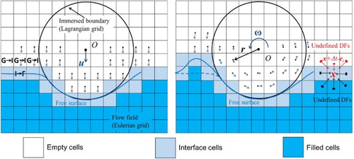
Unlike traditional two-phase flow models that separate fluids by establishing different distribution functions (DFs), the FSLB model only simulates the denser and more viscous phase by the general single-phase LB model, and the free surface is tracked by a special boundary treatment. To simulate free-surface flow by this model, the following assumptions should be made (Körner et al., 2005): (1) the effects of the fluid with lower density and viscosity on another fluid can be neglected; (2) once the state of the simulated fluid is changed, another fluid can reach its equilibrium immediately; (3) a closed layer of the interface cells exists between the simulated fluid cells and the neglected fluid cells. To track the interface, three types of cell, including the filled cell, the interface cell and the empty cell, are introduced (Thürey & Rüde, 2009). The interface can be captured via calculating the fluid fraction ϵ of each cell, which is defined as ϵ = m/ρ, with m being the fluid mass content and ρ being the fluid density. Among all the cells, the filled cell is completely full of the simulated fluid, where the definition of variables and the evolution processes are the same as those in the general LB models. The interface cell is partially filled with fluid, while the empty cell does not contain any simulated fluid, as illustrated in Figure 1. It should be noted that only some key aspects and special treatments are described here, and the overall descriptions and algorithm details can be found in Körner et al. (2005).

Figure 1. Velocity correction of the empty cells neighboring an immersed boundary.

2.1.1. Computation of mass flux

The interface motion in this model is achieved by cell type transformation, which results from the computation of mass flux. By applying the divergence theorem to the convective term and conducting discretization in space on uniform lattices, the continuity equation in discrete form can be derived as (Janßen & Krafczyk, 2011) ∂m/∂t + ∑Δm_i = 0, where m_i denotes the mass variation in the ith direction. The mass variation can be easily computed through the two antiparallel particle distribution functions f_i and f_inv(i) by (1) where inv(i) is the inverse direction of i, and A_i is computed according to (2) in which e_i is the unit vector of the ith direction in the LB method, and E, I and F donate the empty cell, interface cell and filled cell, respectively. With a further discretization in time, the mass at lattice node x for the next time step t + Δt may be expressed as: (3) where n is the number of velocity directions in the LB method. Equation (3) shows that the updated m is calculated by summing the mass variations in all velocity directions. It can be proved that the mass of the flow field updated by Equation (3) is explicitly conserved (Thürey & Rüde, 2009).

2.1.2. Reconstruction of the interface cells

In this algorithm, the filled cell is surrounded by the filled or the interface cells with full set of DFs. However, the interface cell is always adjacent to the empty cells, where the DFs are not defined, and the interface movement cannot be accurately simulated if the DFs of the empty cell enter into the interface cell. In the present algorithm, the missing DFs of the interface cell are reconstructed based on the force balance for opposite lattice directions. Therefore, the reconstructed DFs of interface cell at with empty cell located at can be expressed as (4) where u is the velocity of the cell at position x and time t, and ρ_G = 1 as the pressure is continuous across the interface. In Equation (4), we make use of the fact that forces exerted by the gas are known and are given by the gas pressure and interface velocity. It should be noted that not only the missing DFs but all the DFs with n·e_i < 0 are reconstructed to balance the forces. Vector n denotes the surface normal direction and can be calculated by the second-order central difference approximation . Refer to Thürey and Rüde (2009) for more details about the reconstruction of the interface cell’s DFs.

2.1.3. Mass allocation and interface motion

The interface cell needs to be treated after updating its mass m and fluid fraction ϵ. If the updated fluid fraction ϵ is greater than 1, this interface cell is conversed into a filled cell, and the surrounding empty cells need to be converted into the interface cells. In this step, the new emerging interface cell gains its mass from the surrounding new filled cells, and its density and velocity are assigned to the averaged density and velocity of the neighboring fluid and interface cells. The DFs of the new interface cells can be initialized by the equilibrium distribution function . Likewise, an interface cell should be transformed into an empty cell if its fluid fraction drops below zero, and the surrounding filled cells need to be converted into the interface cells. The negative mass of this interface cell is compensated by the surrounding interface cells and filled cells. As the conversion of cell types is completed, the interface moves, as shown in Figure 1.

To simulate the gravity driven flows, an additional body forcing term H_i should be added to the LB equation. The present model adopts Cheng’s approach (Cheng & Li, 2008) to include the gravity, because it has been proven to be accurate and stable in treating both external force and source terms.

2.2. The immersed boundary method

The basic idea of the IB method using direct forcing approach is briefly described here. Firstly, let the uppercase letters denote Lagrangian variables defined on immersed boundary, and the lowercase letters denote Eulerian variables defined on fluid nodes. The governing equations for fluid flows may be expressed as (Peskin, 2002) (5) (6) (7) (8) (9) where X, F and U are Lagrangian boundary position, boundary force and moving speed, respectively. x, f, u, p and ν are the Eulerian spatial coordinate, external force, flow velocity, pressure, fluid density and viscosity, respectively. (q, r, s) is the Lagrangian curvilinear coordinates of the boundary. Equations (5) and (6) are the N–S equations with external force f in Eulerian form for the fluid flow in domain Ω_f, while Equations (7), (8) and (9) are the IB dynamic equations in Lagrangian form for the boundary Γ_b. The interaction of the fluid and the immersed boundary is realized by the Dirac delta function δ(r) in Equations (7) and (9), in which the former one is used to spread the boundary force F to the nearby fluid nodes and the latter one is used to impose the flow velocity u onto the boundary. S_f is the boundary force generation operator, which is constructed by the direct forcing approach described as follows.

First, the N–S equations are solved by the standard LB model without the external force, and the resulting velocity field is used to obtain the intermediate boundary velocity U* by two-dimensional Lagrangian interpolation (Niu, Shu, Chew, & Peng, 2006). Then, the boundary force defined on each IB point can be calculated by (10) where U_d is the desired boundary velocity and Δt is the time step. It is worth noting that this additional step can be implemented in a very efficient manner, because the collision step in the LB model does not change the macroscopic velocity, and the velocity only needs to be computed in the vicinity of the IB. For more details about the direct-forcing IB method, please see Dupuis, Chatelain, and Koumoutsakos (2008).

2.3. Key treatments of the coupling scheme

2.3.1. Iterative force-correction LB-IB coupling

In the IB method, the boundary forces need to be accurately calculated to realize the non-slip boundary condition on the IB, otherwise fluid could penetrate the boundary and jeopardize the simulation stability. However, the velocity on the IB point may not satisfy the non-slip boundary condition accurately if the direct forcing based IB method is applied, as indicated in literature (Wang, Fan, & Luo, 2008).

To enforce the non-slip boundary condition on the boundary, the IB speed, which is interpolated from the local fluid velocity, should coincide with the actual velocity of the immersed structure. Following Zhang’s work (Zhang, Cheng, Zhu, & Wu, 2016), the aforementioned LB-IB coupling method is improved by the iterative force-correction, in which the boundary force is iteratively calculated to enforce the non-slip boundary condition, assuming that , , and are the intermediate boundary speed, boundary force, Eulerian body force and fluid velocity, where the superscript n denotes the time level while the subscript s denotes the iteration cycle within each time level. First, by solving the N–S equations with the direct-forcing IB method, we obtain the velocity field u₁ⁿ⁺¹, where the subscript 1 represents exerting the direct forcing for the first time. Then, the velocity on the boundary point can be computed by interpolation (11) However, the resulting boundary speed often deviates from the desired speed U_d, and the non-slip boundary condition cannot be satisfied. To alleviate this problem, the directing forcing is exerted for the second time as (12) then the boundary force is spread to the flow field by the Dirac delta function (13) and the velocity of the fluid flow is corrected according to (14) Thus the intermediate boundary speed at iteration cycle s = 2 becomes (15) The is expected to be closer to the desired boundary speed than that of . After several implementations of this procedure within one time step, the boundary speed that is interpolated from the flow field will get much closer to the desired speed and the non-slip boundary condition can thus be enhanced. More details about the iterative force-correction based IB method and its implementation can be found in Zhang et al. (2016).

2.3.2. Velocity correction in the empty cells

The FSLB model only simulates the denser and more viscous phase, and no physical quantity is defined in the empty cells. The IB speed needs to be interpolated from the local fluid velocity as indicated by Equations (7), (11) and (15). However, if the zero velocities of the empty cells that are adjacent to the target IB points are used for this interpolation, the resulting IB speed would deviate from its actual value, which would jeopardize the numerical stability and cause blow-up of simulation.

To alleviate this problem, we introduce a new correction procedure. The velocities of the empty cells, which are imposed onto the target IB points as indicated by Equation (7), are assigned according to the motion of the rigid body. For example, the velocity of the empty cell should be assigned to u if the rigid body translates at the given velocity u. In general, the velocity of the empty cell can be given as u + ω × r, where ω is the angular velocity of the rigid body and r is the vector starting at the mass center of the rigid body and ending at the empty cell, as shown in Figure 1.

2.4. Coupling procedures of the FSLB-IB scheme

A summary of the FSLB-IB coupling scheme with iterative force-correction and velocity correction is as follows. Within each coupling cycle, an iteration process is needed to enforce the non-slip boundary conditions. Given all the variables at time step n, the procedures for marching these variables to the next time step n + 1 are as follows.

1. Compute the IB force F_n+1 from X_n+1 by the direct forcing approach described in Section 2.2.

2. Obtain the Eulerian body force f_n+1 by spreading the IB force F_n+1 to the nearby fluid using Equation (9).

3. Perform LB propagation with the boundary conditions, and calculate the density ρ_n+1 and fluid velocity u_n+1.

4. Calculate the mass flux Δm_n+1 and track the interface movement by using Equations (1), (2) and (3).

5. Reconstruct the DFs in the empty cells by using Equation (4).

6. Advance the DFs in all cells from to by performing the LB collision with the Eulerian body force .

7. Correct the velocity field u_n+1 by the iterative force-correction algorithm (the velocity correction procedure needs to be adopted here).

8. Re-initialize cell types and distribute the excess mass in new filled cells.

9. Initialize the DFs in the new interface cell as detailed in Section 2.1.3.

It should be pointed out that although the algorithm described above is only capable of simulating the one-way coupling FSI problems in which the motion of the immersed object is prescribed, it can be easily extended to the two-way coupling FSI simulations by adding the dynamic equations of rigid objects into the present coupling framework.

3. Validation

To validate the feasibility and accuracy of the proposed FSLB-IB coupling scheme, two typical hydraulic problems, namely the broad-crested weir flow and the sluice gate flow, are simulated. Key qualifications examined in this section include the following: (1) the streamlines could not penetrate the IB; (2) the non-slip boundary conditions on the IB should be enhanced; (3) the difference between the simulated discharge coefficients and those obtained by empirical formulae should be small enough to meet engineering requirements. If not otherwise stated, the fluid viscosity ν = 10⁻⁶ m²/s and gravitational acceleration g = 9.8 m/s² are applied, and the number of Lagrangian points used to discrete the IB is determined in such a way that the distance between two adjacent points is less than half of the Eulerian grid spacing.

3.1. Broad-crested weir flow

The numerical setup is schematically shown in Figure 2. The tunnel is 5.5 m long and 1.25 m high. The weir (2.0 m long and 0.5 m high) is placed 1.5 m behind the flow entrance. In this case, the IB is completely submerged in water, and the iterative force correction treatment can be validated by examining whether the non-slip boundary condition is satisfied.

Figure 2. Flow patterns of the broad-crested weir flow when the water level H = 1.0 m. (a) Pressure distribution; (b) Velocity magnitude and streamlines.

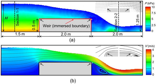
Neglecting the fluid viscosity and applying the continuity equation and Bernoulli’s equation to Sections 1.1 and 2.2, the discharge Q past the broad-crested weir can be calculated via (Hager & Schwalt, 1994) (16) where σ and b are the discharge coefficient and channel width, respectively. The gross water head H₀ is defined as , where H, α, g and υ₀ are the upstream water level, kinematic energy correction coefficient, gravitational acceleration and mean flow rate, respectively.

The simulations are conducted on a uniform lattice 550 × 125. The fixed water level inflow boundary condition (BC) and zero-gradient outflow BC (for details, see(Tang, Li, & Wang, 2008) are applied to the left and right boundaries, respectively; the bottom of the computational domain is treated as non-slip wall, of which the redlines are realized by the proposed IB method while the black lines are handled by the bounce-back boundary scheme described in He, Zou, Luo, and Dembo (1997). Considering different upstream water levels, a series of discharge coefficients can be obtained and then compared with the empirical solutions from the following equation (Hager & Schwalt, 1994): (17) where P is the weir height.

In this case, the weir is completely submersed, and the streamlines would penetrate the weir if the non-slip BC was not enhanced. The water leakage would disturb the neighboring water flow and the local conservation of mass could no longer be satisfied, which would result in incorrect velocity vectors, penetrated stream lines and incorrect discharge coefficients. Therefore, the comparison between the simulated discharge coefficient and the one from Equation (17) can validate the key treatments introduced in Section 2.3.

Figure 2 shows the flow patterns over the weir when H = 1.0 m. For a clear demonstration, the velocity vectors and streamlines around the weir are plotted at the top-right corner of Figure 2(a) and (b), respectively. It can be seen that water smoothly flows over the weir top and the streamlines do not penetrate the weir surface, which indicates that the local conservation of mass is well satisfied, and the non-slip BC is enforced by the proposed coupling scheme. In Figure 3, the simulated discharge coefficients are compared with those obtained by Equation (17), in which the relative error for discharge coefficient E_m is defined as the relative difference between the simulated and empirical results. It can be seen that the simulated discharge coefficients match the empirical solution well, with maximum relative error 4.45%, which is acceptable for engineering applications.

Figure 3. Comparison of the discharge coefficients between the simulated results and empirical solution. The water level is normalized by the weir height P.

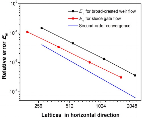
To study the grid convergence of the present coupling scheme, we keep the normalized parameters fixed and refine the fluid lattice and boundary grid. The relative errors for the discharge coefficients are shown in Figure 4, with the upstream water level fixed at H = 1.0 m. Generally speaking, the nearly second-order convergence with surprisingly small errors is evident. Note that this convergence analysis is a rough estimation of grid dependence, because the empirical solutions are used for comparison, which may not be rigorous in itself.

Figure 4. Spatial convergence order for the broad-crested weir flow.

3.2. Sluice gate flow

The sluice gate flow is also typical in hydraulics and has been extensively studied. In this case, the IB will have direct contact with the free surface, meaning that there will be emptied cells residing in the support of IB points during the interpolation process, and the velocity correction treatment can thus be validated. The empirical formula for computing the channel flux is (Tsai, Yen, & Lin, 2002) (18) where e and ϵ are the height of the orifice located at the gate bottom and vertical contraction coefficient, respectively.

The computational setup is shown in Figure 5(a). We use 400 × 150 lattice to conduct the simulations. The BCs are similar to the previous case, and the gate surface is treated as non-slip boundary using the IB method. Four upstream water levels (H = 0.8, 1.0, 1.2, 1.35 m) are simulated, and the discharge coefficients are compared with the following empirical solution (Tsai et al., 2002): (19) The pressure and velocity magnitude of the sluice gate flow with water level H = 0.8 m are shown in Figure 5. It can be seen that the flow field is quite complex and the hydraulic jump can be clearly observed at the downstream end. The simulated sluice gate always contacts with the moving free surface, which demonstrates the good quality of treating the sharp gate edge where the free surface and the IB intersect. Similarly, the velocity vectors and streamlines in the vicinity of the orifice are plotted at the top-right corner of Figure 5(a) and (b), respectively. We can see that the velocity vectors are all parallel to the gate edge and vanish as it approaches the IB surface. No streamlines are found penetrating the IB, which shows good characteristics of the proposed treatments for handling the non-slip boundary condition. The discharge coefficients from the present simulations and the empirical formula (Equation (19)) are shown in Figure 6. In general, the accuracy of the proposed coupling scheme is satisfying, with maximum relative error 3.37%, which is good enough for simulating engineering applications. In addition, the grid convergence characteristics for this case are also shown in Figure 4. A similar second-order convergence is obtained, which is consistent with that of the previous case.

Figure 5. Flow patterns of the sluice gate flow with upstream water level H = 0.8 m. (a) Simulation setup and pressure distribution; (b) Velocity magnitude and streamlines.

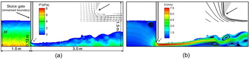
Figure 6. Comparison of the discharge coefficients between the simulated results and empirical solution by considering different water levels.

These two cases tell us that the proposed FSLB-IB coupling scheme can accurately simulate steady flows in practical hydraulic applications.

4. Simulation of hydraulic characteristics of an inclined overflow gate

In this section, the validated coupling scheme is used to analyze the discharge capacity and flow patterns of an inclined overflow gate under stationary and moving conditions.

4.1. Flow patterns and discharge coefficients for different opening angles

A typical example of the overflow gate flow is illustrated in Figure 7. Similarly, the flux Q can be given by Equation (16), where the discharge coefficient σ is used to estimate the discharge capacity of the gate. Following the Pi Theorem, σ can be expressed as σ = ϕ(R_e, θ, L/H₀), indicating that the discharge coefficient is closely related to the Reynolds number Re of the incoming flow, opening of the gate θ and the dimensionless length of the gate L/H₀, where L is the gate chord length. In this section, the relationship between θ and σ is studied in detail by the proposed coupling scheme.

Figure 7. Simulation setup of the inclined overflow gate.

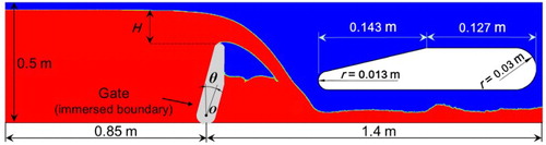
The numerical setup is shown in Figure 7. The simulations for different upstream water levels are performed on a 1125 × 250 uniform lattice. We find that if a coarser grid resolution is applied, the resulting lattice viscosity would be too small to guarantee the stability condition. On the other hand, the present resolution seems to be enough to provide accurate discharge coefficients at relatively low computational costs. The fixed water level inflow BC and the zero-gradient outflow BC are imposed at the left and right side of the domain, respectively.

The bottom is treated as non-slip wall, and the gate is implemented by the IB method. The upstream water level H = 0.15 m, water kinematic viscosity ν = 1.0 × 10⁻⁶ m²/s and gravity g = 9.8 m/s² are applied.

Figure 8 shows the streamlines and velocity magnitude under different openings, when the flow field reaches its steady state. When the gate opening is relatively large, the incoming flow is blocked by the gate and a vortex is formed at the gate front, as indicated by Figure 8 (a, b), which is similar to the lid-driven cavity flow at large Re number. The vortex becomes smaller and eventually disappears as the opening θ increased from 0° to 30°, as shown in Figure 8 (a–c), as the streamlines in the vicinity of the gate will be more aligned with the main stream direction when the gate opening angle decreases. After flowing over the gate top, the water flow falls off under the action of gravity. The velocity magnitude at the downstream end decreases as the gate opening increases, as the larger the gross water head at the up-stream end, the more the static water head can be transferred to the water kinetic energy. When the opening θ = 45°, the horizontal span of the trajectory bucket is the longest, which is beneficial to the stable and safe operation of the gate as the erosion effects of the water flow on the channel and the gate base are reduced. When θ > 70°, the gate is completely submersed in water and the gate flow is similar to the broad-crested weir flow.

Figure 8. Flow patterns of the gate flow under different openings. The left group shows the velocity magnitude and streamlines. The right group shows the pressure distribution.

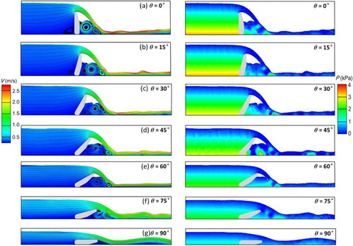
Figure 9 compares the simulated discharge coefficient with data from physical model (Lei et al., 2013). We can find that the simulated σ agrees well with the experimental value, with maximal error 6.34%. The discharge coefficient increases until θ = 30^o, when it reaches the peak. After that it gradually decreases until the gate is completely fallen (θ = 90^o).

Figure 9. Comparison of the discharge coefficients between the simulated results and physical model data.

4.2. Flow patterns and discharge characteristics during the opening process

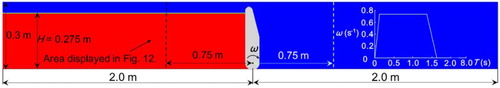
Finally, the opening process of this inclined overflow gate is studied. The water level is fixed at H = 0.275 m. The similar numerical setup as that used in the previous simulation is applied. The gate opening varies from 0° to 60°, and the angular velocity of the gate is prescribed with its time-dependent function, given at the right side of Figure 10.

Figure 10. Simulation setup of the opening process of the inclined overflow gate. The angular velocity of the gate is a function of time.

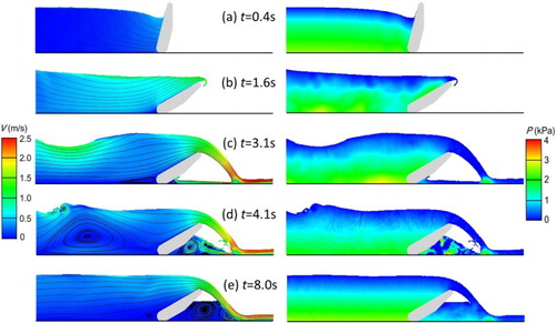
The opening process of this gate and the flow field at some typical times are shown in Figure 11. It should be pointed out that only the region closed by the dashed lines in Figure 10 is plotted. At t = 0.4 s, due to the water pressure acting upon the left surface of the gate, the gate is pushed in the clockwise direction, and a gravitational wave is found traveling in the upstream direction (Figure 11 (a, b)). Then, the gate reaches its maximum opening angle and stops rotating at approximately t = 1.6 s. The water eventually flows over the top tip of the gate and forms a jet body, ast indicated by Figure 11 (c–e). Under the inertia effects, the free surface is elevated to and reaches its peak at t = 3.1 s, as shown in Figure 11 (c). At the same time, the falling water begins to pound on the back of the gate, and a huge vortex is formed in the wake. At the back of the gate, the flow patterns are quite complex, which might cause the gate to vibrate and jeopardize the stability of the hydraulic structure. At last, the free surface becomes horizontal and the whole flow field reaches steady state, as shown in Figure 11 (e).

Figure 11. Flow patterns of the gate opening process at typical times. The left group shows the velocity magnitude and streamlines. The right group shows the pressure distribution.

5. Conclusion and discussion

An FSLB model is firstly coupled to the IB method in this paper to simulate free-surface flow and FSI problems with rapid boundary motion. To enforce the non-slip boundary condition on the IB, an iterative force-correction procedure, proposed in Zhang et al. (2016), is adopted to correct the IB force. To ensure the consistence of the IB velocity interpolation process, the velocity of the empty cells adjacent to the IB is assigned according to the motion of the immersed structure. These two treatments overcome the defects of the coupling scheme. The feasibility and accuracy of the coupling scheme for simulating hydraulic problems are validated by the broad-crested weir flow and sluice gate flow. Finally, as a first attempt at simulating the hydrodynamic applications, the coupling scheme is applied to simulate and analyze both the stationary flow field and the dynamic opening process of an inclined overflow gate. The results demonstrate that the FSLB-IB coupling scheme can accurately simulate realistic hydraulic problems and has good prospects in engineering applications.

It should be pointed out that the present work does not apply local mesh refinement or any wall model to resolve the boundary layer near the IB, which could limit its use in modeling turbulent boundary layers. Actually, the methods that combine the IB method with turbulence and wall models to resolve the high Reynolds number flows have been proposed in some publications. Up to now, the most promising alternative seems to be the combination of the IB method with the large eddy simulation (LES) technique, for which readers may find many of its preliminary applications in Cristallo and Verzicco (2006). The main difficulty lies in the fact that, even with the LES, resolving the finest turbulence structure near the wall still requires a mesh resolution comparable to that of a direct numerical simulation (DNS). In fact, while using a body fitted grid, it is relatively easy to cluster grid nodes in the wall normal direction to meet the above requirement, but the same clustering by a regular Cartesian grid requires refinement in all directions.

Because applying the proposed method to practical applications requires a large amount of grid node while still maintaining the computational efficiency, future work may focus on enhancing the code execution efficiency by means of parallel computing. Moreover, we will try to add some grid techniques such as adaptive mesh refinement to the current method to improve its near wall resolution. By doing so, one can lay the foundation for the extension to the simulations of high Reynolds number flows.

Disclosure statement

No potential conflict of interest was reported by the authors.

Additional information

Funding

This work was supported by the National Natural Science Foundation of China (NSFC), [grant number 10572106], [grant number 10872153], [grant number 11172219] and [grant number 51579187], the Specialized Research Fund for the Doctoral Program of Higher Education of China [grant number 20130141110013], Chongqing Research Program of Application Foundation and Advanced Technology [grant number cstc2016jcyjA1935], Science and technology project of Chongqing Education Committee [grant number KJ1600514] and Open Fund Project of Key Laboratory for Inland Waterway Regulation Engineering of Ministry of communication in Chongqing Jiaotong University [grant number NHHD-201505].

References

- Bertrand-Krajewski, J.-L., Campisano, A., Creaco, E., & Modica, C. (2005). Experimental analysis of the Hydrass flushing gate and field validation of flush propagation modelling. Water Science & Technology A Journal of the International Association on Water Pollution Research, 51(2), 129–137.
- Cheng, Y., & Li, J. (2008). Introducing unsteady non-uniform source terms into the lattice Boltzmann model. International Journal for Numerical Methods in Fluids, 56(6), 629–641. doi: 10.1002/fld.1543
- Cristallo, A., & Verzicco, R. (2006). Combined immersed boundary/large-eddy-simulations of incompressible three dimensional complex flows. Flow, Turbulence and Combustion, 77(1), 3–26. doi: 10.1007/s10494-006-9034-6
- Dupuis, A., Chatelain, P., & Koumoutsakos, P. (2008). An immersed boundary–lattice-Boltzmann method for the simulation of the flow past an impulsively started cylinder. Journal of Computational Physics, 227(9), 4486–4498. doi: 10.1016/j.jcp.2008.01.009
- Hager, W. H., & Schwalt, M. (1994). Broad-crested weir. Journal of Irrigation and Drainage Engineering, 120, 13–26. doi: 10.1061/(ASCE)0733-9437(1994)120:1(13)
- He, X., Zou, Q., Luo, L. S., & Dembo, M. (1997). Analytic solutions of simple flows and analysis of nonslip boundary conditions for the lattice Boltzmann BGK model. Journal of Statistical Physics, 87(1), 115–136. doi: 10.1007/BF02181482
- Janßen, C., & Krafczyk, M. (2011). Free surface flow simulations on GPGPUS using the LBM. Computers & Mathematics with Applications, 61(12), 3549–3563. doi: 10.1016/j.camwa.2011.03.016
- Kim, Y., & Peskin, C. S. (2006). 2–D parachute simulation by the immersed boundary method. Siam Journal on Scientific Computing, 28(6), 2294–2312. doi: 10.1137/S1064827501389060
- Körner, C., Thies, M., Hofmann, T., Thürey, N., & Rüde, U. (2005). Lattice Boltzmann model for free surface flow for modeling foaming. Journal of Statistical Physics, 121(1), 179–196. doi: 10.1007/s10955-005-8879-8
- Lallemand, P., Luo, L. S., & Peng, Y. (2007). A lattice Boltzmann front-tracking method for interface dynamics with surface tension in two dimensions. Journal of Computational Physics, 226(2), 1367–1384. doi: 10.1016/j.jcp.2007.05.021
- Lei, M. H., Nie, R. H., Liu, J. F., & Liu, X. N. (2013). Research on the mixed discharge capacity of new hydraulic flap gate. Journal of Sichuan University, 45(Supp. 2), 47–50. (in Chinese).
- Li, S., & Yang, M. (2012). Numerical simulation of the stability of automatic tilting water gate. Journal of Hydroelectric Engineering, 31(1), 136–139. (in Chinese).
- Mcqueen, D. M., & Peskin, C. S. (2000). A three-dimensional computer model of the human heart for studying cardiac fluid dynamics. ACM SIGGRAPH Computer Graphics, 34(1), 56–60. doi: 10.1145/563788.604453
- Niu, X. D., Shu, C., Chew, Y. T., & Peng, Y. (2006). A momentum exchange-based immersed boundary-lattice Boltzmann method for simulating incompressible viscous flows. Physics Letters A, 354(3), 173–182. doi: 10.1016/j.physleta.2006.01.060
- Peskin, C. S. (1972). Flow patterns around heart valves: A digital computer method for solving the equations of motion (PhD thesis, Physiol.), Albert Einstein Coll. Med., Univ., New York.
- Peskin, C. S. (2002). The immersed boundary method. Acta Numerica, 11, 479–517. doi: 10.1017/S0962492902000077
- Tang, B., Li, J., & Wang, T. (2008). Single-phase lattice Boltzmann model for free-surface flow. Journal of Tsinghua University (Science and Technology), 48(11), 2017–2020.
- Thürey, N., & Rüde, U. (2009). Stable free surface flows with the lattice Boltzmann method on adaptively coarsened grids. Computing and Visualization in Science, 12(5), 247–263. doi: 10.1007/s00791-008-0090-4
- Tian, F. B., Luo, H., Zhu, L., Liao, J. C., & Lu, X. Y. (2011). An efficient immersed boundary-lattice Boltzmann method for the hydrodynamic interaction of elastic filaments. Journal of Computational Physics, 230(19), 7266–7283. doi: 10.1016/j.jcp.2011.05.028
- Tryggvason, G., Bunner, B., Esmaeeli, A., Juric, D., Al-Rawahi, N., Tauber, W., & Jan, Y. J. (2001). A front-tracking method for the computations of multiphase flow. Journal of Computational Physics, 169(2), 708–759. doi: 10.1006/jcph.2001.6726
- Tsai, C. T., Yen, J. F., & Lin, C. H. (2002). Influence of sluice gate contraction coefficient on distinguishing condition. Journal of Irrigation & Drainage Engineering, 128(4), 249–252. doi: 10.1061/(ASCE)0733-9437(2002)128:4(249)
- Wang, M. (2005). Study of hydraulic characteristics of an inclined overflow gate (Ph.D., thesis). Hohai University, Nan Jing.
- Wang, Z., Fan, J., & Luo, K. (2008). Combined multi-direct forcing and immersed boundary method for simulating flows with moving particles. International Journal of Multiphase Flow, 34(3), 283–302. doi: 10.1016/j.ijmultiphaseflow.2007.10.004
- Wu, J., Cheng, Y., Zhang, C., & Diao, W. (2015). Three-dimensional simulation of balloon dynamics by the immersed boundary method coupled to the multiple-relaxation-time lattice Boltzmann method. Communications in Computational Physics, 17(5), 1271–1300. doi: 10.4208/cicp.2014.m385
- Zhang, C., Cheng, Y., Zhu, L., & Wu, J. (2016). Accuracy improvement of the immersed boundary–lattice Boltzmann coupling scheme by iterative force correction. Computers & Fluids, 124, 246–260. doi: 10.1016/j.compfluid.2015.03.024
- Zhang, J., Johnson, P. C., & Popel, A. S. (2007). An immersed boundary lattice Boltzmann approach to simulate deformable liquid capsules and its application to microscopic blood flows. Physical Biology, 4(4), 285–295. doi: 10.1088/1478-3975/4/4/005
- Zhang, Y., Feng, Y., Yi, W., Liu, X., & Li, K. (2010). Experimental study on the discharge coefficient of hydraulic flap gate. Journal of Hydroelectric Engineering, 29(5), 220–225. (in Chinese).