Rough boundary treatment method for the shear-stress transport k - ω model

ABSTRACT

Most of existing rough boundary treatment methods for the shear-stress transport model require much finer grids than smooth boundary treatment methods. Knopp, Eisfeld, and Calvo (2009, A new extension for k–ω turbulence models to account for wall roughness. International Journal of Heat and Fluid Flow, 30(1), 54–65.) developed a rough boundary treatment method that allows the same grid resolution as smooth boundary treatment methods, but its effect of grid resolution on the computed velocity is strong. This study aims to improve the method of Knopp et al. (2009, A new extension for k–ω turbulence models to account for wall roughness. International Journal of Heat and Fluid Flow, 30(1), 54–65.) and to reduce the effect of grid resolution. This work newly incorporates the effect of grid resolution on boundary values of , the inverse time scale. The method generates the logarithmic velocity profile of open channel flows over rough beds with a velocity shift relative to that over smooth beds. The computed velocity shift, depending on the dimensionless roughness, generally agrees with the measured ones. The effect of the grid resolution on velocity shift that is computed using the present method is only 31% of that using the method of Knopp et al. (2009, A new extension for k–ω turbulence models to account for wall roughness. International Journal of Heat and Fluid Flow, 30(1), 54–65.) in the transitionally rough regime. The effect of grid resolution in the transitionally rough regime is stronger than in both the hydraulically smooth regime and the fully rough regime. The present method is applied to simulate open channel flow over a bed with suddenly changing roughness. The computed velocities are consistent with the measured ones. The method reveals a sharp response of the shear velocity to the sudden change in roughness.

KEYWORDS:

• RANS model
• rough boundary
• open channel flows
• SST model

1. Introduction

Roughness elements on surfaces disturb flow and change near-bed turbulence characteristics (Flack & Schultz, 2014; Schultz & Flack, 2007). The mean velocity profile and the friction coefficient for a rough surface, therefore, differ from those for a smooth surface (Jiménez, 2004). Examples of flow over rough surfaces include open channel flows, atmospheric flows over complex terrain, and flows in industrial piping systems. In hydraulic engineering, accurately predicting open channel flow is important, and requires the effective modeling of the effect of roughness.

The ratio of the roughness height, , to the viscous length scale, where  = the shear velocity and  = the kinematic viscosity, quantifies the effects of roughness on the near-wall turbulence. As the ratio, , increases the flow passes through three regimes, which are (1) the hydraulically smooth regime, (2) the transitionally rough regime, and (3) the fully rough regime (Jiménez, 2004; Schultz & Flack, 2007). In the hydraulically smooth regime, the flow disturbance that is induced by roughness elements is damped out by viscosity, so the roughness elements do not significantly affect the flow. In this regime, the flow structure over a rough surface is, then, identical to that over a smooth surface. The flow comprises three layers near surface, which are, in order of increasing distance from the wall, (1) a viscous sublayer in which viscous effects dominates, (2) a buffer layer in which both viscosity and turbulence are important and which is responsible for generating turbulent energy (Robinson, 1991), and (3) a log-law layer in which turbulence dominates and the flow has a logarithmic velocity profile. In the hydraulically smooth regime, the roughness elements are within the viscous sublayer. The drag on the roughness elements is dominated by the shear stress. In the fully rough regime, the roughness element destroys the flow structure in the sublayer and the buffer layer, and the roughness importantly affects the flow. The flow has also a logarithmic velocity profile but with a negative velocity shift; in other words, the logarithmic velocity profile is preserved but velocity over a rough wall is smaller than velocity over a smooth wall. The drag on the roughness element is dominated by the pressure. The transitionally rough regime is between the other two regimes. The flow in the transitionally rough regime exhibits a shifted logarithmic velocity profile. Both the pressure and the shear stress on the roughness element are important. The upper and lower limits of for the transitionally rough regime are not well understood. The upper limit can range from 55 to 90 and the lower limit ranges from 2.5 to 9; those values depend on the composition of the surface (Flack, Schultz, & Rose, 2012; Nikuradse, 1933).

In the last two decades, various numerical approaches that solve Reynolds-Averaged Navier-Stokes equations have been widely used to study open channel flows. These approaches depend on a turbulence model to compute the turbulence kinetic energy, , the inverse time scale of turbulence, , and the eddy viscosity. The shear-stress transport (SST) model, developed by Menter (1992), is a popular model that is successfully used to simulate a wide range of turbulent flows (Goldberg & Batten, 2015; Hu, Li, Han, Cai, & Xu, 2016; Nieto, Hargreaves, Owen, & Hernandez, 2015). The SST model reduces to the model (Launder & Spalding, 1974) in the free stream layer and to the model (Wilcox, 1988) close to the wall. The SST model inherits the advantages of both of these models without their disadvantages.

Some boundary treatment methods that consider the effects of rough surface on turbulence for the SST model are available. Their main purpose is not to reflect in detail the characteristics of turbulence but to capture the resulting shift of the logarithmic velocity profile. The first method is based on a wall function that combines analytic solutions for the sublayer and log-law layers (Apsley, 2007). The constraint is , with  = distance from the first cell center to the wall, which must exceed (Eça & Hoekstra, 2011). For complex flows over rough surfaces, the grid must be sufficiently fine to resolve the complex flows, but the condition may not be satisfied. The second method is based on Wilcox’s proposal to compute on the surface (Wilcox, 2008). Wilcox’s proposal applies only to the model; Hellsten and Laine (1997) proposed an eddy-viscosity limiter to extend Wilcox’s proposal to the SST model. The disadvantage of the second method is the unreasonably small to be used. For >150, is required, but for the hydraulically smooth regime yields sufficient fineness (Knopp, Eisfeld, & Calvo, 2009). Additionally, the second method cannot be applied when the roughness is very large. To overcome the limitations of the second method, Knopp et al. (2009) related the and boundary values to based on a proposal concerning the eddy viscosity in the log-law layer, which can yield a logarithmic profile; in their method, suffices, but the computational results are highly grid-dependent. Furthermore, the method of Knopp et al. (2009) performs poorly in the transitionally rough regime. Having analyzed the second and third methods, Aupoix (2014) proposed a fourth method, which performs well in the three roughness regimes, but the method requires a very fine grid.

At present, there does not exist a rough boundary method that does not require too fine a grid and without strong effect of grid resolution on computational results. This study improves the method of Knopp et al. (2009) and reduces the effect of the grid resolution by considering the grid resolution on boundary values. This work does not address the other weakness of the method of Knopp et al. (2009) concerning the poor performance in the transitionally rough regime; in that regime, the velocity shift depends on the composition of the wall and is not well understood. The improved method is applied to open channel flows over a uniformly rough surface and a surface with a suddenly changing roughness.

2. Mathematical formulas

In this study, RANS equations are solved using an open source computational fluid dynamics library, called OpenFOAM. Numerous turbulence models are included in OpenFOAM and can be selected at run time. However, the SST in OpenFOAM differs from that of Menter (1992); the former uses the viscosity limiter that was proposed by Hellsten and Laine (1997) for a rough surface. Following Knopp et al. (2009), the SST model of Menter (1992) is implemented in this study, and briefly summarized in Section 2.1. Section 2.2. presents the improved boundary treatment method.

2.1. Turbulence model

In the SST model (Menter, 1992), and are determined by solving (1) and (2) where  = velocity, with , with , is a blending function, and other undefined terms (, ,,,,) are model parameters. goes to 1 in the inner layer, so Equations (1) and (2) reduce to the corresponding equations in the model. goes to 0 in the outer layer and Equations (1) and (2) reduce to the corresponding equations in the model. The turbulent viscosity, , is calculated as (3) where is a constant and . depends on the distance to the wall, ; in the inner layer and in the outer layer. The difference between and is that falls off to zero well within the inner layer but at the edge. In the model, is computed as . The limitation on in Equation (3) is based on Bradshaw’s assumption that the principal turbulent stress is proportional to (Menter, 1992); this limitation improves the performance of the model for boundary layer flows with an adverse pressure gradient. Table 1 presents the model coefficients. According to Menter (1992), the first term on the right-hand-side of Equation (2) is , where . For incompressible flow (=0), becomes and it is mathematically consistent of .

Table 1. Coefficients in SST model.

	0.31
	0.09
	with and
	with and
	with and
	with and

2.2. Rough boundary treatment

This work improves the method of Knopp et al. (2009) by considering the effect of grid resolution on boundary values of . The method of Knopp et al. (2009) is briefly reviewed, and then its improvement is presented.

2.2.1. Method of Knopp et al.

The method of Knopp et al. (2009) is based on the ideas of Aupoix and Spalart (2003) and Durbin, Medic, Seo, Eaton, and Song (2001), in which the eddy viscosity in the log-law layer is computed by (4) where is the shear velocity, is the von Karman constant, is the distance to the wall, and is related to the hydraulic roughness length. By the eddy viscosity hypothesis, is expressed by (5) where is the velocity parallel to the boundary. Equations (4) and (5) together with the no-slip boundary condition yield the logarithmic velocity profile (6) For a fully rough wall, Aupoix and Spalart (2003) suggested , and Equation (6) is consistent with the experimentally observed velocity profiles. Under fully rough conditions, the viscous sublayer is completely disrupted; with respect to modeling, Knopp et al. (2009) proposed that the value of at the wall should be close to the log-law layer value, and so (7) Together, Equation (4) and suggest (8) It is worth mentioning that Knopp et al. (2009) used but not Equation (3) when deriving Equation (8). Equations (7) and (8) are only applicable in the fully rough regime. To extend the boundary treatment method to the other two regimes: the hydraulically smooth regime, where and at the wall (Wilcox, 1988), and the transitionally rough regime, Knopp et al. (2009) used two blending functions, such that (9) and (10) where is the distance from the first cell center to the wall, and (11) As mentioned in the introduction, the advantage of the method of Knopp et al. (2009) is that a coarser grid () than used in the methods of Wilcox (2008) and of Aupoix (2014) can be used. However, the computed velocity using the method of Knopp et al. (2009) depends strongly on the grid resolution, and can be improved by considering the grid resolution in Equation (4). In the origin method of Knopp et al. (2009), the second term in of Equation (10) is , but this study finds that give better results than for .

2.2.2. Improvement

To consider the effect of grid resolution, Equation (5) is discretized to yield (12) Then, Equation (6) is substituted into Equation (12), yielding (13) Unlike Equation (4), Equation (13) accounts for the grid resolution. Equation (7) is used to compute at the wall, and yields at the wall of (14) When ,  Equation (14) reduces to Equation (8). When is too small, the value of computed by Equation (14) may exceed ; this yields smaller than that for the smooth wall. This is unreasonable. To avoid too small , I followed Knopp et al. (2009) to add a limiter into Equation (14): (15) In summary, in this work, Equations (9) and (15) are used to compute and at the wall. These two equations reduce to those for a smooth surface when is very small. Sine Equation (6) is derived for flows in the log-law layer with zero pressure gradient, Equation (15), which is proposed based on Equation (6), may be inapplicable to flow separation problems. Previous studies have suggested that should be used in the first grid cell and at the wall for the smooth wall (Wilcox, 1988). Here, at the wall gave better results than when using the grid resolution of .

3. Open channel flow with uniform roughness

The proposed method is used to study open channel flow over uniform roughness, which is depicted schematically in Figure 1. The flow depth is set to m and the energy slope is . To cover the three flow regimes, a range of from 1 to 600 is adopted. The computational domain is . The entire computational domain is filled with water with and . Gradient of , , and are set to zero at the upper boundary. The periodic boundary condition is imposed in the direction. The no-slip boundary condition and the proposed method for determining and are used at the bed. Various grid systems are adopted here. All the grid systems are expanded from the bed with an expansion ratio of 1.1 in the direction, but various is used; varies from 0.5 to 10. All of the grid cells have the same size in the direction; the width of each grid cell is 0.01 m. The numbers of the grid cells are from 20 × 56 () to 20 × 116 (). In computations, an OpenFOAM built-in solver ‘pimpleFOAM’ is adopted. OpenFOAM is based on the finite volume method. Many discretization schemes and linear solvers can be selected at run time. This study used the Crank-Nicolson time scheme. The convection terms are discretized by the ‘Gauss upwind’ scheme; the diffusion terms by the ‘Gauss linear’ scheme; the gradient derivative terms by the ‘Gauss linear’ scheme. A preconditioned bi-conjugate gradient solver is adopted to solve the linear equations from the equations governing , , and . The equation governing the hydrodynamic pressure is solved using a preconditioned conjugate gradient method. For details of the schemes and the solvers, please refer to the book of Moukalled, Mangani, and Darwish (2016).

Figure 1. Uniform open channel flow.

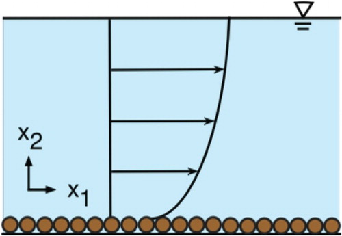
Figure 2 presents the computed velocities for  = 1 (hydraulically smooth regime), 40 (transitionally rough regime), and 100 (fully rough regime). Figure 2 superposes (1) the linear velocity profile of the sublayer (16) where is a constant, and , and (2) the logarithmic velocity profiles of the log-law layer (17) where is a constant. The values of and in Figure 2 are obtained by regression analyses. To compute , the computed velocity profiles in the region of are used; to obtain , the computed velocity profiles in the region are used. Figure 2 demonstrates that the computed velocities match the linear velocity profiles that are given by Equation (16) at and they are consistent with the logarithmic velocity profiles that are given by Equation (17) at . The value of declines from to 0.42 as increases. Previous studies have suggested in the hydraulically smooth regime and in the transitionally rough regime. In the fully rough regime, no measurement of velocity can be made. The velocity profile in the log-law layer is shifted to the left. A larger yields a larger , as is observed experimentally (Nikuradse, 1933). The variations of and with are discussed below.

Figure 2. Velocity profiles for open channel flows with three kinds of roughness. The values of and are obtained by the regression analyses.

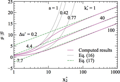
Figure 3 plots the variations in the computed with and . Figure 3 superposes the measured from various types of roughness, including sandpaper (Flack, Schultz, & Connelly, 2007), pyramids (Schultz & Flack, 2009), honed (Schultz & Flack, 2007), and packed spheres (Schultz & Flack, 2005); the equivalent sand grain roughness height, which is related to the root-mean-square roughness height and the skewness of the roughness surface elevation, is used here to calculate , as suggested by Flack and Schultz (2014). Figure 3 also plots the formula that was proposed by Nikuradse (1933) for uniform sand, based on experimental results. In Figure 3, the computed agrees well with for uniform sand in the fully rough regime (Nikuradse, 1933) where, say, . The relationship between and changes with the type of roughness. However, when the equivalent sand grain roughness height is used, the relationships for various types of roughness become identical (Flack & Schultz, 2014). The effect of the grid on the computed velocity profiles is negligible in the fully rough regime, as revealed by Figure 3. In the transitional rough regime, say , the deviation of the computed from for the uniform sand (Nikuradse, 1933) is considerable and the grid effect is significant. In this regime, different types of roughness yield different , even when the equivalent sand grain roughness height is used (Flack & Schultz, 2014). The computed values of are within the range of measured except when . For engineering purposes, the proposed model can be used in the transitionally rough regime for because the uncertainty that is caused by the grid resolution is of the same order of magnitude as that by the type of roughness. In the hydraulically smooth regime, the proposed method reduces to the method of Wilcox (1988) for a smooth wall. The computed values of are close to zero for ; for , is overestimated while for , is underestimated.

Figure 3. Velocity shift obtained using present method and experimentally for different and .

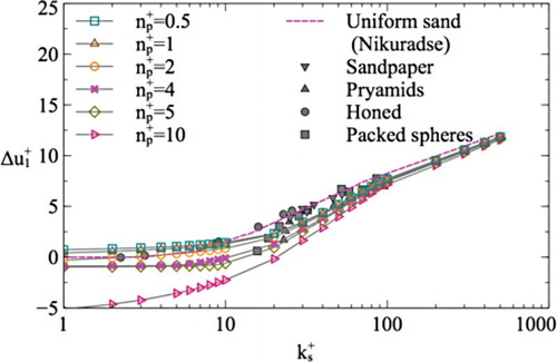
Figure 4 displays values that were computed using the method of Knopp et al. (2009). Figures 3 and 4 reveal that the present method and the method of Knopp et al. (2009) perform similar to each other. In both methods, effects of grid resolution are observed at , but in the present method, the effect of the grid resolution is weaker, especially at . To compare carefully the effects of grid resolution, Figure 5 plots as a function of for 1, 20, and 100, covering the three flow regimes. For (fully rough regime), the effect of the grid resolution that is generated by the present method is insignificant, and the variation of is less than 0.5%. It is greater than the method of Knopp et al. (2009), by which the variation in is 36%. The effect of grid resolution at (transitionally rough regime) is more significant than that at . The that is computed using the present method changes from 2.33 (for  = 1) to −0.17 (for  = 10), whereas that computed using the method of Knopp et al. (2009) changes from 1.99 to −6.13. The former change is only 31% of the latter. At , the effects of grid resolution that are generated by both methods are almost equal because both methods reduce to that of Wilcox (1988) when is very small. As discussed before, this work improves upon the method of Knopp et al. (2009) in the fully rough regime, and this improvement is realized by considering the grid resolution on the boundary value of . However, in this work, the blending function of Knopp et al. (2009) for the transitional rough regime and the hydraulically smooth regime is also used, possibly explaining why the method herein largely eliminates the grid effect in the fully rough regime but only slightly reduces the grid effect in the transitionally rough regime.

Figure 4. Velocity shift obtained using method of Knopp et al. (2009) for different and .

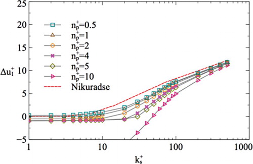
Figure 5. Comparison of velocity shifts obtained by present method and method of Knopp et al. (2009) with various grid resolutions for 1, 20, and 100.

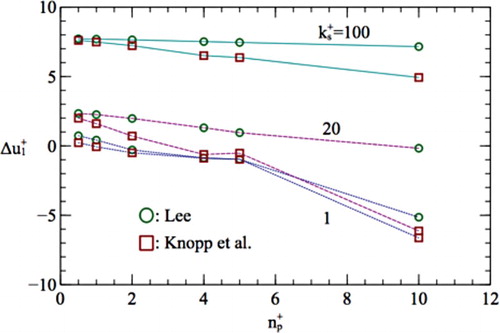
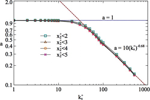
Figure 6 plots versus . To check whether is affected by the regions that are considered in the regression analysis, four regions are used; and similar results are obtained, as presented in Figure 6. Figure 6 reveals that when , is unity. The value of decreases monotonically as increase above 10 and approaches at . As mentioned in the Introduction, some works (Apsley, 2007) blended Equation (16) with and Equation (17), and used the resulting function to compute the near-wall velocity, which is adopted in OpenFOAM. Such a method does not consider the effect of roughness on and so breaks down when the grid is too fine. The relationship between and , displayed in Figure 6, may be useable to improve the method.

Figure 6. Variation of with by the regression analysis.

This study developed a new rough boundary treatment method. Three similar methods were developed by Hellsten and Laine (1997), Knopp et al. (2009), and Aupoix (2014). The methods of Hellsten and Laine (1997) and Aupoix (2014) require very fine grids, . In the method of Knopp et al. (2009), suffices but their computational results are highly grid-dependent. This study improves the method of Knopp et al. (2009) and reduces the effect of grid solution on computational results. The grid-resolution effect of the present model can be 31% of the method of Knopp et al. (2009). With the present boundary treatment method, the required near-wall resolution can be relaxed to approximately . The improvement is restricted to cases in the transitionally rough regime and the fully rough regime.

4. Open channel flow with step change in roughness

In a natural open channel, such as stream or river, the roughness of the bed is not always uniform. The proposed method is used to simulate open channel flow with a step change in roughness, as depicted schematically in Figure 7. In this work, the only applied flow conditions are depth, , =  m and mean transverse velocity, , = 0.2 . The roughness upstream, , is m and that downstream, , is m. The computational domain is . The step change occurs at 8 downstream of the inlet. The width of the grid cell is 0.01 m and the height of the grid cell far from the bed is . The height of the first grid cell from the bed is and the grid cells close to the bed are expanded with an expansion ratio of 1.1. The maximum is within 1.2. The number of the grid cells is 1000 × 178. In computations, another OpenFOAM built-in solver ‘interFoam’ is adopted. The adopted discretization schemes and linear solvers are the same as those used in the simulations of open channel flow with uniform roughness. A volume-of-fluid (VOF) method is used to track the interface. The logarithmic velocity profile at the inlet is specified; and are adopted according to Ferziger and Peric (2002). At the outlet, the gradient of velocity, , and are zero. Previous studies (Carravetta & Morte, 2004) have suggested that , which is the distance between the top surfaces of the two roughness elements, is an important parameter. In this study, a flat theoretical bed is assumed, located at approximate blow the roughness elements (Liu, 2014) where the mean velocity is zero. Therefore, is approximately m.

Figure 7. Open channel flow over rough bed with step change in roughness.

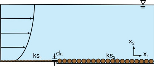
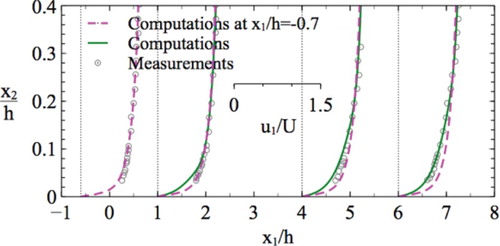
Figure 8 plots the computed velocity profiles at  = −0.7, 1, 4, and 6. The origin of the axis is located at the step change in roughness. Figure 8 superposes the measurements of velocity using a micro acoustic Doppler velocimeter (Chen & Chiew, 2003). The experiment of Chen and Chiew (2003) was conducted in a glass-sided horizontal flume that was 30 m long, 0.7 m wide, and 0.6 m deep. The flow with free surface was driven by gravity and it was fully developed before it passed over the location of change of bed roughness (16 m from the upstream end of the flume). In the experiment of Chen and Chiew (2003), m is set, which is different from of m, adopted here. This study tried to lower the bed to make m, yielding a backward-facing step. The backward-facing step leaded to flow separation, influencing bed shear stress. To show how the velocity field responses to the sudden change of the bed roughness, the computed velocity at  = −0.7 is copied and moved to the locations of  = 1, 4, and 6 for comparison purpose. As presented in Figure 8, the computed velocity profiles are adjusted at . The flow decelerates in the region close to the bed, and this region becomes larger as increases, forming an internal boundary layer. The velocity slightly increases far from the bed, maintaining constant discharge. Although the proposed method somewhat underestimates the velocity at , the computed velocity profiles are generally consistent with the measured ones, validating the present model.

Figure 8. Velocity profiles at  = −0.7, 1, 4, and 6. To show how the velocity responses to the sudden change of the bed roughness, the computed velocity at  = −0.7 is copied and moved to the locations of  = 1, 4, and 6 for comparison purpose.

Here the shear velocity is examined. The shear velocity can be directly computed (Method 1) as (18) and two other methods for computing it are available. One is based on regression analysis and Equation (17), and uses the velocity at , as in Chen and Chiew (2003) (Method 2). The other uses the equation (Method 3), (19) which is widely used in turbulence computations. In computing using Equation (19), at is used. Figure 9 shows the results that are obtained using the three methods. Figure 9 superposes two experimentally obtained shear velocities (Chen & Chiew, 2003); one is obtained using the measured velocity and regression analysis with Equation (17) (Method 4) and the other is obtained from the measured Reynolds stress near bed (Method 5). Table 2 summarizes the five methods herein for computing . Among Methods 1–3, Method 1, used in numerical computation of the open channel flow, provides the ‘true’ shear velocity. Figure 9 reveals that Method 1 yields a sharp response of at but Methods 4 and 5 yield gentle responses. Some studies (Nezu & Tominaga, 1994) have also found sharp responses. Methods 2 and 3 yield gentle responses, unlike Method 1, suggesting that the regression analysis with Equation (17) and Equation (19), included in Methods 2–4, cannot be used here, possibly because Equations (17) and (19) are applied to fully developed flow but not under transitional conditions. Furthermore, the turbulence varies rapidly close to the bed, and using turbulence properties at different locations to estimate yields very different results. Therefore, turbulence properties (adopted in Methods 3 and 5) may not be useable to estimate here. Some previous studies (Nezu & Tominaga, 1994) have revealed an overshooting of shear velocity to peak close to and downstream of the step change in roughness but others have not. Carravetta and Morte (2004) found that the overshoot may occur for large , but this phenomenon is not well understood. The proposed model cannot change arbitrarily. Thus, this model cannot be applied to examine overshooting.

Figure 9. Shear velocities for flow over rough bed with step change in roughness. Measurements are digitized from Chen and Chiew (2003).

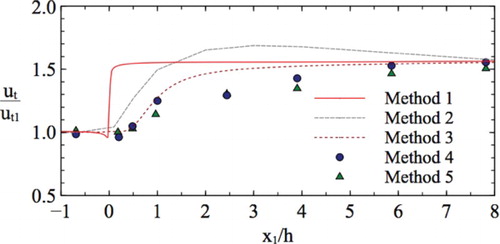
Table 2. Summary of five methods used to determine .

	Method 1	Method 2	Method 3	Method 4	Method 5
Data origin	Computation	Computation	Computation	Measurement	Measurement
Approach	Eq. (18)	Regression analysis	Eq. (19)	Regression analysis	Reynolds stress

5. Conclusions

This work improves upon the rough boundary treatment method of Knopp et al. (2009) for the SST model. The effect of grid on velocity that is derived from the logarithmic velocity profile is considered in the boundary condition of . The improved method is applied to solve two problems related to open channel flows – one with uniform roughness and the other with a step change in roughness.

For uniform roughness, the computed velocity shift, which declines as the dimensionless roughness increases, is generally consistent with previous experimental observations (Chen & Chiew, 2003). The effect of the grid resolution on the computed results is reduced. In the transitionally rough regime, the variation in the computed velocity shift with grid resolutions () that is obtained by the proposed method is only 31% of that obtained by the method of Knopp et al. (2009).

With the step change in roughness (two kinds of roughness), the proposed method can generate velocity profiles that are consistent with previous measurements. The shear velocity obtained directly from the computational bed shear stress responds sharply to the change in roughness. However, two additional methods, unlike that based on shear stress, yield gentle responses of shear velocity; one is based on the regression analysis of the computed velocity profile and the other based on turbulent kinetic energy and a formula that is widely used in turbulence computations. A possible reason for this difference is that these two methods apply in the local equilibrium state. Therefore, they cannot be used to compute shear velocity for flow over a suddenly changing roughness.

With the present boundary treatment method, the required near-wall resolution can be relaxed to approximately , but the improvement is restricted to cases in the transitionally rough regime and the fully rough regime. The present method may be inapplicable to flow separation problems; this needs further tests and improvement. In the future, the present method will be applied to scour simulations.

Disclosure statement

No potential conflict of interest was reported by the author.

Additional information

Funding

This work was supported by Ministry of Science and Technology, Taiwan: [Grant Number MOST 105- 2218-E-032-001-].

References

- Apsley, D. (2007). CFD calculation of turbulent flow with arbitrary wall roughness. Flow, Turbulence and Combustion, 78(2), 153–175. doi: 10.1007/s10494-006-9059-x
- Aupoix, B. (2014). Roughness corrections for the k–ω shear stress transport model: Status and proposals. Journal of Fluids Engineering, 137(2), 1–10. doi: 10.1115/1.4028122
- Aupoix, B., & Spalart, P. R. (2003). Extensions of the spalart-allmaras turbulence model to account for wall roughness. International Journal of Heat and Fluid Flow, 24, 454–462. doi: 10.1016/S0142-727X(03)00043-2
- Carravetta, A., & Morte, R. D. (2004). Discussion of “response of velocity and turbulence to sudden change of Bed roughness in open-channel flow” by xingwei chen and Yee-meng chiew. Journal of Hydraulic Engineering, 130(6), 587–589. doi: 10.1061/(ASCE)0733-9429(2004)130:6(587)
- Chen, X. W., & Chiew, Y. M. (2003). Response of velocity and turbulence to sudden change of bed roughness in open-channel flow. Journal of Hydraulic Engineering, 129(1), 35–43. doi: 10.1061/(ASCE)0733-9429(2003)129:1(35)
- Durbin, P. A., Medic, G., Seo, J. M., Eaton, J. K., & Song, S. (2001). Rough wall modification of two-layer k-ε. Journal of Fluids Engineering, 123(1), 16–21. doi: 10.1115/1.1343086
- Eça, L., & Hoekstra, M. (2011). Numerical aspects of including wall roughness effects in the SST k-ω eddy-viscosity turbulence model. Computers and Fluids, 40(1), 299–314. doi: 10.1016/j.compfluid.2010.09.035
- Ferziger, J. H., & Peric, M. (2002). Computational methods for fluid dynamics. Berlin: Springer.
- Flack, K. A., & Schultz, M. P. (2014). Roughness effects on wall-bounded turbulent flows. Physics of Fluids, 26(10), 1–17. doi: 10.1063/1.4896280
- Flack, K. A., Schultz, M. P., & Connelly, J. S. (2007). Examination of a critical roughness height for outer layer similarity. Physics of Fluids, 19(9), 1–9. doi: 10.1063/1.2757708
- Flack, K. A., Schultz, M. P., & Rose, W. B. (2012). The onset of roughness effects in the transitionally rough regime. International Journal of Heat and Fluid Flow, 35, 160–167. doi: 10.1016/j.ijheatfluidflow.2012.02.003
- Goldberg, U. C., & Batten, P. (2015). A wall-distance-free version of the SST turbulence model. Engineering Applications of Computational Fluid Mechanics, 9(1), 33–40. doi: 10.1080/19942060.2015.1004791
- Hellsten, A., & Laine, S. (1997). Extension of the k-ω-SST turbulence model for flows over rough surfaces. 22nd atmospheric flight mechanics conference, guidance, navigation, and control and co-located conferences AIAA Paper (pp. 1–9). New Orleans, LA, USA.
- Hu, P., Li, Y., Han, Y., Cai, S. C. S., & Xu, X. (2016). Numerical simulations of the mean wind speeds and turbulence intensities over simplified gorges using the SST turbulence model. Engineering Applications of Computational Fluid Mechanics, 10(1), 359–372. doi: 10.1080/19942060.2016.1169947
- Jiménez, J. (2004). Turbulent flows over rough walls. Annual Review of Fluid Mechanics, 36(1991), 173–196. doi: 10.1146/annurev.fluid.36.050802.122103
- Knopp, T., Eisfeld, B., & Calvo, J. B. (2009). A new extension for k–ω turbulence models to account for wall roughness. International Journal of Heat and Fluid Flow, 30(1), 54–65. doi: 10.1016/j.ijheatfluidflow.2008.09.009
- Launder, B. E., & Spalding, D. B. (1974). The numerical computation of turbulent flows. Computer Methods in Applied Mechanics and Engineering, 3(2), 269–289. doi: 10.1016/0045-7825(74)90029-2
- Liu, X. (2014). New near-wall treatment for suspended sediment transport simulations with high reynolds number turbulence models. Journal of Hydraulic Engineering, 140(3), 333–339. doi: 10.1061/(ASCE)HY.1943-7900.0000824
- Menter, F. R. (1992). Improved two-equation k-omega turbulence models for aerodynamic flows. NASA STI/Recon Technical Report N.
- Moukalled, F., Mangani, L., & Darwish, M. (2016). The finite volume method in computational fluid dynamics - An advanced Introduction with OpenFOAM and matlab. Berlin: Springer.
- Nezu, I., & Tominaga, A. (1994). Response of velocity and turbulence to abrupt changes from smooth to rough beds in open-channel flow. Proc., symposium on fundamentals and advancements in hydraulic measurements and experimentation, Buffalo, New York, 195–204.
- Nieto, F., Hargreaves, D. M., Owen, J. S., & Hernandez, S. (2015). On the applicability of 2D URANS and SST turbulence model to the fluid-structure interaction of rectangular cylinders. Engineering Applications of Computational Fluid Mechanics, 9(1), 157–173. doi: 10.1080/19942060.2015.1004817
- Nikuradse, J. (1933). Laws of flow in rough pipes. Berlin: NACA Technical Memorandum 1292.
- Robinson, S. K. (1991). Coherent motions in the turbulent boundary layer. Annual Review of Fluid Mechanics, 23(1), 601–639. doi: 10.1146/annurev.fl.23.010191.003125
- Schultz, M. P., & Flack, K. A. (2005). Outer layer similarity in fully rough turbulent boundary layers. Experiments in Fluids, 38(3), 328–340. doi: 10.1007/s00348-004-0903-2
- Schultz, M. P., & Flack, K. a. (2007). The rough-wall turbulent boundary layer from the hydraulically smooth to the fully rough regime. Journal of Fluid Mechanics, 580, 381–405. doi: 10.1017/S0022112007005502
- Schultz, M. P., & Flack, K. A. (2009). Turbulent boundary layers on a systematically varied rough wall. Physics of Fluids, 21, 1–9. doi: 10.1063/1.3059630
- Wilcox, D. C. (1988). Reassessment of the scale-determining equation for advanced turbulence models. AIAA Journal, 26(11), 1299–1310. doi: 10.2514/3.10041
- Wilcox, D. C. (2008). Formulation of the k-w turbulence model revisited. AIAA Journal, 46(11), 2823–2838. doi: 10.2514/1.36541