Viscous numerical wave tank for Bragg resonance by cnoidal and Stokes waves

ABSTRACT

In this study, a quadtreeadaptive viscous numerical wave tank in which the free surface is resolved by the volume of fluid method is established to solve Bragg resonance caused by Stokes and cnoidal waves. Numerical wavemakers of third-order cnoidal and fifth-order Stokes waves are implemented. Additionally, a numerical damping zone is implemented such that the numerical grid in that area is automatically coarsened under a prescribed low resolution in which the time-matching is more efficient without an excessively small time-step. Furthermore, the areas with intense vorticity, boundary layers, and free surfaces are automatically refined to prescribed high resolutions. The model is shown as stable even when multiple adaptation () criteria are implemented in the computation. With respect to the simulation of Bragg resonance caused by Stokes waves, the obtained reflection and transmission coefficients, velocity in the boundary layers as well as velocity and vorticity fields are compared with other results obtained by extant studies. The model is then applied for solving Bragg resonance caused by cnoidal waves which show stronger scouring on the lee side of the submerged obstacles. The numerical results exhibit higher resolution for examining the secondary eddies compared with the conventional numerical methods. In addition, the computing time of the model with an adaptive grid is at least six times faster than that with a semi-uniform grid while their results are in a good agreement.

KEYWORDS:

• Computational fluid dynamics
• quadtree–adaption
• volume of fluid
• numerical damping zone
• Stokes Bragg resonance
• cnoidal Bragg resonance

1. Introduction

A numerical wave tank (NWT) is the computational counterpart of a wave flume that corresponds to a physical tank with length that significantly exceeds other dimensions. In an NWT, the wave motion is simulated either by an inviscid model (Brorsen & Larsen, 1987; Senturk, 2011; Tanizawa, 1996) or a viscous model (Anbarsooz, Passandideh-Fard, & Moghiman, 2013; Lin & Liu, 1999). Predominantly, several applications of wave interactions were explored by a potential-theory-based NWT. Wang, Tang, and Wu (2016) explored the issue of the wave–body interactions for a surface-piercing barge by DBIEM (Wang, Tang, & Wu, 2015). They indicate that the forces of first harmonics decrease with increases in the pitch moment. Typically, the viscous NWT is modeled by using the Navier–Stokes equations and are more suitable for simulating flow conditions with significant eddies in the wave motions. Essentially, the Navier–Stokes equations are solved by the finite difference method (Park, Kim, & Miyata, 1999), finite element method (Ramaswamy & Kawahara, 1987), or finite volume method (Bai, Mingham, Causon, & Qian, 2010). Additionally, the free surfaces are mostly resolved by the level set method (Bihs & Kamath, 2017) or the volume of fluid (VOF) method (Hirt & Nichols, 1981).

To improve the efficiency of the prescribed methods of static meshes, it is necessary to focus on the development of novel algorithms to more efficiently solve the governing equations of physically-complicated flows with free surfaces. A method to reduce the computational cost of solving these problems involves using the adaptive mesh refinement. Examples include the adaptive unstructured meshes with the level set method (Xie et al., 2014; Zheng, Lowengrub, Anderson, & Cristini, 2005) as well as structured meshes with hybrid level set/front tracking methods (Ceniceros, Roma, Silveira-Neto, & Villar, 2010) and with the quadtree adaptation and VOF method (Popinet, 2003, 2009, 2013). The last method was applied to several problems in engineering and science (Cimpeanu & Papageorgiou, 2014; Dasgupta, Tomar, & Govindarajan, 2015; Deike, Melville, & Popinet, 2015; Deike, Popinet, & Melville, 2015; Dietze, 2016; Li, Li, Zong, & Chen, 2014; Tsai, Hou, Popinet, & Chao, 2013). In this study, the quadtree–adaptive solver is applied to study the Bragg resonance by a viscous NWT that is composed of a numerical wavemaker at one end and a numerical damping zone at the other end to restrict wave reflections.

Bragg resonance for water waves was examined by several studies in experimental investigations or numerical simulations. A simple row of breakwaters produces a nature water wall in front of the first submerged structure to dissipate wave energy. Several researchers followed this idea in experimental and numerical efforts as reported in international journals. For example, Cho, Lee, and Kim (2004) experimentally investigated a strong Bragg reflection given the issue of regular wave propagation. Hsu et al. (2007) used a second-order fully non-linear Boussinesq type model to explore Bragg reflection of irregular waves. Tsai, Kuo, Lan, Hsu, and Chen (2011) investigated the Bragg scattering of multiply composite artificial bars and validated their results by using the EEMSE model (Hsu, Tsai, & Huang, 2003). However, linear theoretical and numerical predictions are limited to the potential assumptions used. Tsai, Lin, Chang, and Hsu (2016) developed a coupled-mode eigenfunction matching method to investigate the Bragg reflection of weak viscous waves under a linear wave assumption. In order to further observe hydrodynamic details with respect to surroundings of breakwaters, Hsu et al. (2014) investigated vortex evolution during Bragg renounce caused by a Stokes wave. They obtained numerical results by using the COBRAS model (Lin & Liu, 1998) and indicated that a shift of reflection at the primary resonance occurred due to non-linear, viscous, and turbulence effects.

The present study involves establishing a quadtree–adaptive viscous NWT to examine the Bragg resonance caused by the Stokes and cnoidal waves. Numerical wavemakers with 3rd cnoidal and 5th Stokes waves as well as a numerical damping zone are implemented. The damping zone is designed such that the numerical grid is sufficiently coarse to enable an efficient time-matching without an excessively small time-step. Furthermore, the areas with intense vorticity, boundary layers, and free surfaces are automatically refined to prescribed high resolutions. The model is shown as stable even when multiple adaptation criteria are considered in the computation. In addition, the computing time of the model with an adaptive grid will be shown to be of the same accuracy but much higher efficiency compared with the model with a semi-uniform grid. To compare our results for the Stokes Bragg resonance with those obtained by extant studies (Hsu et al., 2014), we also use the NWT to study the Bragg resonance caused by cnoidal waves.

This paper is organized as follows. In Section 2, a viscous NWT is established by the quadtree–adaptive solver. Specifically, a higher order wave making boundary is simply added with known conditions of initial velocities. A dynamic quadtree–adaptive grid automatically provides an immediate improvement with respect to grid treating. Additionally, a numerical wavemaker and a damping zone are introduced. The numerical results and validations are given in Section 3. Finally, the conclusions are presented in Section 4.

2. Viscous numerical wave tank

2.1. Quadtree–adaptive flow solver

Popinet (2003) created a general-purpose spacetree–adaptive solver to analyze multi-phase fluid flows with interfaces resolved by the VOF method. The two-dimensional and three-dimensional flow problems are solved by using quadtree and octree, respectively. Subsequently, an algorithm was developed to include the effect of surface tension (Popinet, 2009). A short review on the flow solver for solving two-dimensional problems is provided. We consider a two-phase flow problem of air and water, and the governing Navier–Stoke equations based on an incompressible assumption with variable density (Deike, Melville, et al., 2015; Deike, Popinet, et al., 2015; Popinet, 2009; Popinet, 2009) are given as follows: (1) (2) (3) where denotes the two-dimensional fluid velocity, denotes the volume fraction with an interval value from 0 to 1, is defined as the strain tensor, denotes pressure, and denote coupled kinematic viscosity and fluid density with respect to , respectively, and denotes a term of the surface tension. Then the surface elevation is defined as . In addition, and denote the kinematic viscosities for water and air, respectively. This is similar for and . Additionally, Eq. (2) is an advection–density equation. Numerically, we denote if a grid cell is full of air. Conversely, represents that a grid cell is full of water. In order to focus on the interface, the reduced gravity model is utilized while considering the surface tension force.

After the governing equations are introduced, the projection method (Chorin, 1968) can be applied to obtain a second-order accurate time discretization on Eqs. (1)–(3). In the projection method, the viscous terms of the discretized momentum equation are efficiently treated by the second-order accurate Crank–Nicolson method. Furthermore, the density and the velocity advection terms in Eqs. (2) and (3), respectively, are solved by the second-order unsplit upwind scheme (Bell, Colella, & Glaz, 1989). As a result, the velocity is governed by a vector-valued Helmholtz equation. Additionally, and are obtained by solving scalar Poisson and Helmholtz equations, respectively. The numerical stability satisfies the following limitations (Johnston & Liu, 2004): (4) where and denote the local grid size and time-step, respectively.

With respect to the spatial discretization, the equations are solved by using the quadtree based multilevel solver that is described in detail in a previous study (Popinet, 2003). A typical quadtree grid is depicted in Figure 1. Furthermore, second order accuracy is considered in the spatial discretization. More details on the flow solver are given in the previous studies (Popinet, 2003, 2013). The treatment of the surface tension is also given in extant studies (Deike, Popinet, et al., 2015; Popinet, 2009).

Figure 1. A sketch of the adaptive mesh refinement.

2.2. Numerical wavemakers

As depicted in Figure 2, a viscous NWT is implemented with a numerical wavemaker on and a numerical damping zone in . In the figure, denotes the wave height, denotes the wave length with denoting the wavenumber, denotes the water depth, and denotes the trough depth. Additionally, denotes the phase velocity of the wave with denoting the wave period and no current is considered in the study. In numerical experiments, should be set sufficiently large to contain the numerical wave gages and structures but not too large so that the computation are kept efficient.

Figure 2. Schematic diagram of the viscous numerical wave tank.

With respect to , the numerical wavemaker is implemented by setting the following boundary conditions: (5) (6) (7) where and denote the given velocity and water elevation based on the theories of Stokes and cnoidal waves, respectively.

With respect to the Stokes waves, the prescribed boundary conditions are based on fifth-order solutions (Fenton, 1985; Tsai, Chen, & Hsu, 2015). It should be noted that the initial fluid flow is assumed as irrotational and the surface tension effects are neglected. Subsequently, the solutions are as follows: (8) (9) (10) where gives the remainder on division of by 2, denotes the perturbation parameter, and denotes the gravity. The dimensionless coefficients of and are given in previous studies (Fenton, 1985; Tsai et al., 2015).

With respect to the cnoidal wave solutions, the boundary condition is based on the third-order cnoidal solutions of Fenton (1998). The solutions are given as follows: (11) (12) (13) where , , , , and , and correspond to elliptic functions. With respect to a given wave condition (, and given), the parameter of elliptic functions is solved by using the combined equation of Eqs. (24) and (A.2) in Fenton (1998). Thus, we obtain , , and from Eq. (A.8), (A.2), and (A.6), respectively, in Fenton (1998). The dimensionless coefficients of are based on a study by Fenton (1998).

In previous studies (Fenton, 1990, 1998), Fenton proposed a method to distinguish the usage of Stokes or cnoidal wave theory as shown in Figure 3. The Ursell number is defined as follows: (14) In the present implementation of the numerical wavemaker, we use Figure 3 to identify the two theories when a specific wave condition (, and given) is considered. Essentially, the 5th Stokes wave theory is used for . With respect to a longer wave (), the numerical wavemaker is replaced using the 3rd cnoidal wave theory.

Figure 3. A criterion of different wave theories.

2.3. Numerical damping zone

To dissipate the wave energy and avoid secondary wave reflection, a numerical damping zone is conducted in as shown in Figure 2. The elimination of wave reflections at the domain boundaries is commonly achieved by the following:

1. Increasing the domain size

2. Beaches (Lal & Elangovan, 2008): configuring a slope in a zone beside the domain boundary

3. Grid damping (Kraskowski, 2010): Increasing the grid size towards the corresponding domain boundary

4. Active wave absorption techniques (Schäffer & Klopman, 2000): a boundary-based wavemaker generates waves to eliminate incoming waves

5. Damping layer approaches (Ha, Lee, & Cho, 2011; Park et al., 1999): momentum sinks are included in the governing equations to damp the waves propagating through the zone

In the study, we use artificial kinematic viscosity combined with the adapted grid damping to form our numerical damping zone. In the zone, an artificial kinematic viscosity is assumed as a function of location as follows: (15) where (16) Evidently, . In this study, we typically select and . In addition, the maximum refined level in a box is denoted as and the minimum level is defined as (or equivalently the grid of a box is refined to ). In order to ensure the numerical stability and the convergence in computing process, the temporal domain is automatically adjusted as per Eq. (4). To implement the numerical damping zone, we typically set the grid size in the entire damping zone as the minimum level as depicted in Figure 4. If the maximum refined level is otherwise utilized in the damping zone, the time-step should be times smaller as indicated in Eq. (4). As a result, the present implementation of numerical damping zone significantly improves numerical accuracy. Numerical evidence will be given in the next section.

Figure 4. Water surface elevations by a damping zone at various time instants in an empty tank.

2.4. Other adaption criteria

In addition to the adapted damping zone considered in the previous subsection, adaptations of free surface and vorticity are also considered to achieve grid-cost reduction and improvements on the solution accuracy. On the free surface (), the grid size is adapted to the maximum refined level to have a higher resolution of the surface profiles.

In present studies, the simulations are all started with the quiet initial conditions. As time passes, the vorticity generated at the structure boundaries is advected away from the structure and evolves into eddies. Therefore, the computational grid should be adapted dynamically to follow this evolution using the vorticity criterion as (17) where is the threshold value which is interpreted as the maximum acceptable angular deviation defined according to the maximum cell cost, which is typically set to 0.01 in this study. More details can be found in the literature (Popinet, 2003, 2009, 2013).

3. Results and discussions

In this section, we consider the cnoidal Bragg resonance in subsection 3.3 and the Stokes Bragg resonance in the other subsections where the latter NWT is set based on the following configuration. It should be noted that the conditions of the incident waves for the Stokes and the cnoidal Bragg resonances are selected as shown in Figure 3. In the present investigation, a numerical wave tank is established by 90 connected boxes in which each box size is defined as as shown in Figure 5. To construct an environment of simulations, we follow initial settings and conditions in previous studies (Hsu et al., 2014). The mean water depth is 0.12 m; the wave height is 0.032 m; the height of the submerged breakwater is 0.04 m, the width of the submerged breakwater is 0.12 m and the distance of each bar is 0.48 m. In addition to the basic investigations on the free surface, we also observe variations of vortex and investigate velocity profiles in the boundary layer near the breakwaters. Additionally, a simple dissipating mechanic with and as mentioned in subsection 2.3 is implemented. To evaluate the performance of the numerical damping zone, an empty tank is considered by removing the submerged breakwaters in Figure 5. The wave condition is configured according to the Stokes Bragg resonance in subsection 3.2. Using the least squares method (Mansard & Funke, 1980), the reflection coefficient is evaluated to be 2.7% which is similar to the results obtained by a potential-theory-based numerical damping zone (Tanizawa, 1996). Evidently, it is good for wave dissipation without considering the fluid and solid interaction problems. In addition, dynamic grid adaptations on free surface and vorticity as introduced in subsection 2.4 are also implemented. The maximum and minimum refined levels of the dynamic grid adaptations are tabulated in Table 1. In the table, the computing configurations of uniform and semi-uniform grids will be introduced and utilized in subsection 3.4.

Figure 5. Arrangement of the numerical setup and computational domain.

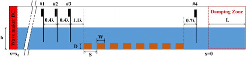
Table 1. Comparisons of the grid level by different types of refinement.

	Water	Free surface	Damping zone	Air
Min/max
levels	and	and		and
Uniform grid
Semi-uniform grid
Dynamic grid adaptation

3.1. Validations

In the beginning of this numerical experiment, we follow the benchmark example of water wave Bragg reflections (Hsu et al., 2014). The Bragg reflections on the free surface are calculated by using the least squares method (Mansard & Funke, 1980), and the velocity profiles are directly estimated by numerical wave gages. Figure 6 mainly shows scattering results that are compared to the results obtained by (Hsu et al., 2014). Specifically, we investigate and add the reflection and transmission of several types of long waves based on cnoidal wave theory. It is observed that the present results are in reasonable agreement with their investigations. It should be noted that the same shift of reflection trend is observed on the primary resonance due to the non-linearity, and thus the shear tress and turbulence effects are captured. It should also be noted that a shift of reflection trend truly occurs in the second resonance. This phenomenon is reasonably revealed by reviewing the Bragg reflections results obtained by Kirby and Anton (1990). To provide additional information to support this argument, the VEMM model (Tsai et al., 2016) is also used to predict a solution of the present case for comparison purposes. The evidences indicate that even in the linear water wave condition, the reflection peak on the second peak also shifts away from a ratio of . Furthermore, explorations of velocity profile under the water surface are implemented, and a complete velocity variation on the vertical direction from the free surface to the bottom is also depicted in Figure 7. Clearly, an overshooting phenomenon can be observed. Overall agreements in terms of velocity profiles between present investigations and the previous results (Hsu et al., 2014) are reasonable.

Figure 6. A comparison of (a) reflections and (b) transmissions of Bragg scattering by water waves over a series of submerged rectangular breakwaters.

Figure 7. Comparisons of velocity profiles of Stokes Bragg resonance (a) before 1st breakwater at and (b) before 1st breakwater at .

3.2. Stokes Bragg resonance

The velocity profile is deformed when a water wave propagates over submerged obstacles. Additionally, vortices are principally formed around the same obstacles due to the quick development of boundary layer. The impact of height/speed vortices causes substantial damage to the surface of artificial obstacles and makes the structure foundation unstable. Figures 8 and 9 show the results of velocity vectors and vorticity contours for the Stokes Bragg resonance () at an accelerating phase and a decelerating phase , respectively. Given the use of dynamic grid adaptations, the results indicate the development of a primary counterclockwise eddy on the top of the first breakwater close to the lee side when a mature wave crest approaches. In contrast, a primary clockwise eddy forms behind the first breakwater when the wave crest passes through the first breakwater (i.e. the next wave trough approaches the first breakwater). These primary eddies are also noted in the literature (Hsu et al., 2014).

Figure 8. Numerical results of (a) vorticity fields, (b) velocity vector fields and (c) adaptive grids at phase for the Stokes Bragg resonance.

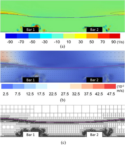
Figure 9. Numerical results of (a) vorticity fields, (b) velocity vector fields and (c) adaptive grids at phase for the Stokes Bragg resonance.

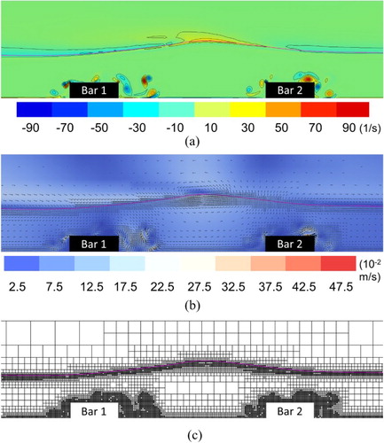
By using the dynamic grid adaptations based on the vorticity intensity, the grid is dynamically refined to capture these eddies as shown in Figures 8cc and 9c. Significantly, secondary counterclockwise eddies can be found at the right of the primary eddies for both cases of the accelerating and decelerating phases. These secondary eddies, however, were not resolved in the previous study (Hsu et al., 2014). Evidently, these eddies result in strong scouring on the lee side of the submerged obstacles.

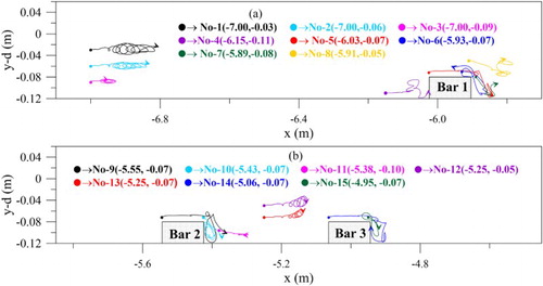
Additionally, tracks of particles movements are depi-cted in Figure 10. In the figure, particles are shown to shift to the downstream with the mass transport when wave trains propagate over a flat topography. Significantly, the trajectories are not closed. Also, the movements of particles are directly relevant to the variations of vortices. The high turbulences of scouring make particle trajectories unstable on the lee side of the submerged obstacles. Briefly, the details of particles tracking are helpful for observations related to the scour, sediment drift, and pollutant diffusion.

Figure 10. A time history distributions ( sec) of particles trajectories at different positions for the Stokes Bragg resonance.

To investigate the viscous effect, a higher viscosity liquid (SAE oil, ) is considered. Other arrangements are kept unchanged. Figures 11 and 12 show the results of velocity vectors and vorticity contours at an accelerating phase and a decelerating phase , respectively. Compared with the results of water waves in Figures 8 and 9, the values of wave heights, velocities and vorticities are much smaller due to the stronger dissipation of the oil. In addition, no eddies can be clearly observed and therefore the scours behind the bars are very mild.

Figure 11. Numerical results of (a) vorticity fields and (b) velocity vector fields at phase for the Stokes Bragg resonance of oil.

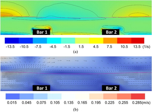
Figure 12. Numerical results of (a) vorticity fields and (b) velocity vector fields at phase for the Stokes Bragg resonance of oil.

3.3. Cnoidal Bragg resonance

In this subsection, fluid motions near the submerged breakwater are investigated when the cnoidal water waves propagate over a series of rectangular breakwaters. To obtain further understanding of the fluid behavior of non-linear long wave at resonance conditions, a large-scale model based on a ratio value of wavelength and bar width is designed for the following simulations. We use the same vertical scale as mentioned in the beginning of this section. The only change is that the horizontal scale is twice that of the setting of the Stokes case. Velocity profiles on the top of the first breakwater and others in front of the first breakwater are compared as shown in Figure 13. Results show that both horizontal velocity profiles are similar except that the horizontal velocity of the cnoidal case is more uniform. However, there are a few differences in terms of the vertical velocity due to the asymmetry wave shape.

Figure 13. Comparisons of velocity profiles between Stokes waves and cnoidal waves under Bragg resonance condition (a) before 1st breakwater and (b) on the top center of 1st breakwater.

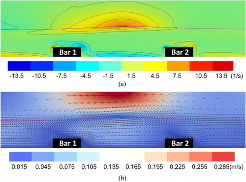
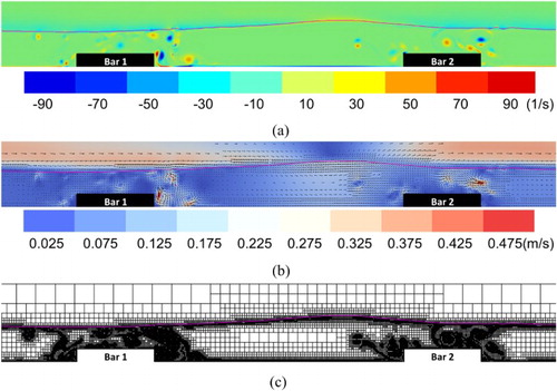
By using the dynamic grid adaptations, Figures 14 and 15 depict the results of velocity vectors and vorticity contours for the cnoidal Bragg resonance at an accelerating phase and a decelerating phase , respectively. In Figure 14, it can be observed that there is a primary counterclockwise eddy on the top of the first breakwater close to the lee side at an accelerating phase. On the other hand, a primary clockwise eddy forms behind the first breakwater when the wave crest passes through the first breakwater. In addition, it can be found that there are multiple secondary eddies at the right of the primary eddies for the decelerating phases. These eddies tend to result in a stronger scouring on the lee side of the submerged obstacles compared with the Stokes Bragg resonance. Correspondingly, the dynamically refined grids for capturing these eddies are given in Figures 14c and 15c.

Figure 14. Numerical results of (a) vorticity fields, (b) velocity vector fields and (c) adaptive grids at phase for the cnoidal Bragg resonance.

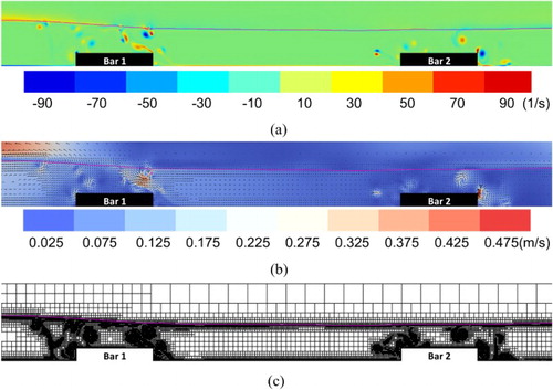
Figure 15. Numerical results of (a) vorticity fields, (b) velocity vector fields and (c) adaptive grids at phase for the cnoidal Bragg resonance.

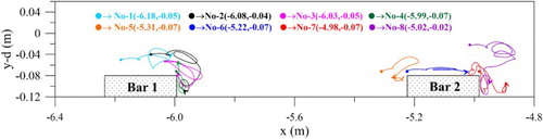
Then, typical particle trajectories of the fluid motion for the cnoidal Bragg resonance are depicted in Figure 16. In the figure, it shows more severe chaotic motions on the lee side of the submerged obstacles compared with those for the Stokes Bragg resonance. This also tends to indicate that the scouring of the cnoidal Bragg resonance is stronger than that of the Stokes Bragg resonance.

Figure 16. A time history distributions ( sec) of particles trajectories at different positions for the cnoidal Bragg resonance.

Lastly, Table 2 shows few parameters that are relevant to wave scattering for the Stokes and cnoidal Bragg resonances. This illustrates that the arrangement of the series submerged breakwaters is a good coastal construction technique to reduce the transmissions of waves coming from the distant sea. Generally, the non-linearity of wave propagation is more relevant and the vorticities are enhanced more severely when comparing the results of cnoidal Bragg resonances to those of the Stokes case. As a result, the energy dissipation of the cnoidal waves is 20% higher than that of the Stokes waves

Table 2. Comparisons of scattering parameters for Stokes and cnoidal Bragg resonances.

Stokes resonance	0.7072	0.5859	15.66%	20.81	29431
cnoidal resonance	0.5956	0.5454	34.78%	83.23	57143

3.4. Computing efficiency

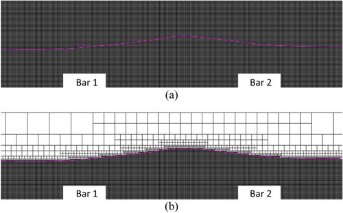
In order to demonstrate the efficiency improvement of the dynamic grid adaptations, we also consider simulations on the Stokes Bragg resonance by using semi-uniform and uniform grids. For the semi-uniform grid, the adaptations on the free surface and in the damping zone are maintained; however, the solutions in the water area are resolved by the maximum refined level of grids. On the other hand, the grid is set to the maximum level in the entire computational domain including the damping zone for the uniform grid. Details for the settings are given in Table 1. Typical grid configurations are given in Figures 17 and 18, respectively, for the accelerating and decelerating phases.

Figure 17. A comparison of (a) uniform and (b) semi-uniform grids at phase for the Stokes Bragg resonance.

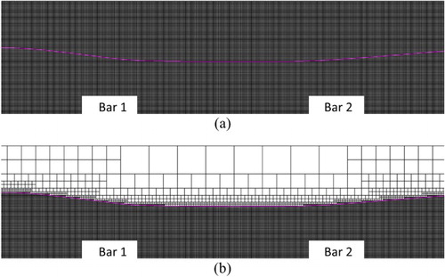
Figure 18. A comparison of (a) uniform and (b) semi-uniform grids at phase for the Stokes Bragg resonance.

In order to realize the efficiency of different usages of adaptations, a parallel test by a high standard work station (Intel® Xeon(R) CPU ES-2620 V3@ 2.4 GHz × 16, 8G memories) is implemented. A comparison of the computational costs is summarized in Table 3 for the simulations of uniform grid, semi-uniform grid, and dynamic grid adaptations. In the table, it can be observed that the acceleration of the simulation by the dynamic grid adaptations over that by the semi-uniform grid is more than six times faster. In order to ensure the accuracy of those results, vorticity contours obtained by the semi-uniform grid are given in Figure 19. Compared with Figures 8 and 9, excellent agreements between the vorticity contours obtained by the dynamic grid adaptations and the semi-uniform grid can be observed. The evidence shows that the results of both cases are reasonable and coincident while the acceleration for the simulation by the dynamic grid adaptations is significant. In other words, the same accurate numerical results can be obtained by using the dynamic grid adaptations with a much higher efficiency compared with those by the semi-uniform grid.

Figure 19. A vorticity contour obtained by a simulation of semi-uniform grid at phases (a) and (b) for the Stokes Bragg resonance.

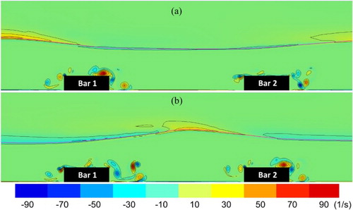
Table 3. Comparisons of grid cost by different type of refinement (physical time: 20 s).

Type of the refined mesh	Number of cells	Computing time (hours)	Speed up	Interval of Time step	Total time step
Uniform grid			–^a	1.31∼1.63 ()
Semi–uniform grid		59.1	^a	0.94∼3.61 ()
			–^b
Dynamic grid adaption		9.82	^a	0.56∼7.23 ()
			^b

^awith respect to uniform grid.

^bwith respect to semi-uniform grid.

For the simulation by the uniform grid, the computing time is estimated to be too long and unrealistic since the damping zone is also resolved by the maximum refined level. According to the explanation in subsection 2.3, to ensure the simulation is stable the time-step for the uniform grid should be times smaller than those of the other two grid settings. As a result, the computing time for the simulation by the uniform grid is about one thousand times longer than that by the other two grid settings as given in Table 3. This demonstrates the efficiency improvement of the proposed adapted damping zone.

4. Conclusions

In this study, a quadtree–adaptive flow solver is used to establish a viscous numerical wave tank. Numerical wavemakers of fifth-order Stokes and third-order cnoidal waves are implemented. To eliminate the reflective waves of the tank, a numerical damping zone is implemented such that the numerical grid is automatically coarsened to the minimum level. Therefore, the time-matching is stable and more efficient without an excessively small time-step as shown by numerical results. The dynamic adaptation model is then applied for solving Bragg resonances caused by both of the Stokes and cnoidal waves. The cnoidal Bragg resonance is shown to have a stronger scouring on the lee side of the submerged obstacles and a 20% higher energy dissipation compared with those of the Stokes Bragg resonance. With the dynamic grid adaptations, the model can resolve not only the primary eddies but also the secondary eddies in which the later ones are not found in a previous study. Numerical results also indicate that the computing time of the model with an adaptive grid is at least six times faster than that with a semi-uniform grid while their results are in a good agreement.

In the near future, the dynamic grid adaptation will become a more popular numerical technique for solving problems in oceanic engineering. For example, the method can be applied for solving three-dimensional wave problems with fluid–structure interactions. This is currently under investigation.

Nomenclature

	=	Dimensionless coefficient of and (–)
	=	Dimensionless coefficient of (–)
	=	Parameter of volume fraction (–)
	=	Elliptic function (–)
	=	Phase velocity
	=	water depth
	=	Elliptic function (–)
	=	strain tensor (–)
	=	gravity
	=	Trough depth
	=	Wave height
	=	Wave number
	=	Length of damping zone
	=	Parameter of elliptic functions and integrals (–)
	=	Maximum refined level in a box (–)
	=	Minimum refined level in a box (–)
	=	Pressure ()
	=	Reflection coefficient (–)
	=	Wave period ()
	=	Transmission coefficient (–)
	=	Elliptic function (–)
	=	Distance between adjacent submerged breakwaters ()
	=	Horizontal component of fluid velocity in domain ()
	=	Horizontal component of fluid velocity at ()
	=	Ursell number (–)
	=	Mean fluid speed in frame of wave ()
	=	Vertical component of fluid velocity at in domain ()
	=	Vertical component of fluid velocity at ()
	=	Expression of shallowness (–)
	=	Quantity used in series for velocity components (–)
	=	Dimensionless water height (–)
	=	Surface elevation in domain ()
	=	Surface elevation at ()
	=	Wave length ()
	=	coupled kinematic viscosity ()
	=	(–)
	=	threshold value of adaptation (–)
	=	coupled fluid density ()
	=	dimensionless coefficients of cnoidal wave velocity (–)
	=	surface tension ()

Disclosure statement

No potential conflict of interest was reported by the authors.

ORCID

Chia-Cheng Tsai http://orcid.org/0000-0002-4464-5623

References

- Anbarsooz, M., Passandideh-Fard, M., & Moghiman, M. (2013). Fully nonlinear viscous wave generation in numerical wave tanks. Ocean Engineering, 59, 73–85.
- Bai, W., Mingham, C. G., Causon, D. M., & Qian, L. (2010). Finite volume simulation of viscous free surface waves using the Cartesian cut cell approach. International Journal for Numerical Methods in Fluids, 63(1), 69–95.
- Bell, J. B., Colella, P., & Glaz, H. M. (1989). A second-order projection method for the incompressible Navier-Stokes equations. Journal of Computational Physics, 85(2), 257–283.
- Bihs, H., & Kamath, A. (2017). A combined level set/ghost cell immersed boundary representation for floating body simulations. International Journal for Numerical Methods in Fluids, 83(12), 905–916.
- Brorsen, M., & Larsen, J. (1987). Source generation of nonlinear gravity waves with the boundary integral equation method. Coastal Engineering, 11(2), 93–113.
- Ceniceros, H. D., Roma, A. M., Silveira-Neto, A., & Villar, M. M. (2010). A robust, fully adaptive hybrid level-set/front-tracking method for two-phase flows with an accurate surface tension computation. Communications in Computational Physics, 8(1), 51–94.
- Cho, Y. S., Lee, J. I., & Kim, Y. T. (2004). Experimental study of strong reflection of regular water waves over submerged breakwaters in tandem. Ocean Engineering, 31(10), 1325–1335.
- Chorin, A. J. (1968). Numerical solution of the Navier-Stokes equations. Mathematics of Computation, 22(104), 745–762.
- Cimpeanu, R., & Papageorgiou, D. (2014). On the generation of nonlinear travelling waves in confined geometries using electric fields. Philosophical Transactions of the Royal Society A: Mathematical, Physical and Engineering Sciences, 372(2020), 1–14.
- Dasgupta, R., Tomar, G., & Govindarajan, R. (2015). Numerical study of laminar, standing hydraulic jumps in a planar geometry. The European Physical Journal E, 38(45), 1–14.
- Deike, L., Melville, W. K., & Popinet, S. (2015). Air entrainment and bubble statistics in three-dimensional breaking waves. Bulletin of the American Physical Society, 60, 1–2.
- Deike, L., Popinet, S., & Melville, W. K. (2015). Capillary effects on wave breaking. Journal of Fluid Mechanics, 769, 541–569.
- Dietze, G. F. (2016). On the Kapitza instability and the generation of capillary waves. Journal of Fluid Mechanics, 789, 368–401.
- Fenton, J. D. (1985). A fifth-order stokes theory for steady waves. Journal of Waterway, Port, Coastal, and Ocean Engineering, 111(2), 216–234.
- Fenton, J. D. (1990). Nonlinear wave theories. the Sea, 9(Part A), 3–25.
- Fenton, J. D. (1998). The cnoidal theory of water waves. In J. B. Herbich (Ed.), Developments in offshore engineering: Wave phenomena and offshore topics (handbook of coastal & ocean engineering) (pp. 55–101). Houston: GulfProfessional Publishing.
- Ha, T., Lee, J., & Cho, Y. S. (2011). Internal wave maker for Navier-Stokes equations in a three-dimensional numerical model. Journal of Coastal Research, 64, 511–515.
- Hirt, C. W., & Nichols, B. D. (1981). Volume of fluid (VOF) method for the dynamics of free boundaries. Journal of Computational Physics, 39(1), 201–225.
- Hsu, T. W., Hsiao, S. C., Ou, S. H., Wang, S. K., Yang, B. D., & Chou, S. E. (2007). An application of Boussinesq equations to Bragg reflection of irregular waves. Ocean Engineering, 34(5–6), 870–883.
- Hsu, T. W., Lin, J. F., Hsiao, S. C., Ou, S. H., Babanin, A. V., & Wu, Y. T. (2014). Wave reflection and vortex evolution in Bragg scattering in real fluids. Ocean Engineering, 88, 508–519.
- Hsu, T. W., Tsai, L. H., & Huang, Y. T. (2003). Bragg scattering of water waves by multiply composite artificial bars. Coastal Engineering Journal, 45(2), 235–253.
- Johnston, H., & Liu, J. G. (2004). Accurate, stable and efficient Navier–Stokes solvers based on explicit treatment of the pressure term. Journal of Computational Physics, 199(1), 221–259.
- Kirby, J. T., & Anton, J. P. (1990). Bragg reflection of waves by artificial bars. Proceedings of the 22nd international conference on coastal engineering, New York.
- Kraskowski, M. (2010). Simulating hull dynamics in waves using a RANSE code. Ship Technology Research, 57(2), 120–127.
- Lal, A., & Elangovan, M. (2008). CFD simulation and validation of flap type wave-maker. World Academy of Science, Engineering and Technology, 46(1), 76–82.
- Li, H. t., Li, J., Zong, Z., & Chen, Z. (2014). Numerical studies on sloshing in rectangular tanks using a tree-based adaptive solver and experimental validation. Ocean Engineering, 82, 20–31.
- Lin, P., & Liu, P. L. F. (1998). Turbulence transport, vorticity dynamics, and solute mixing under plunging breaking waves in surf zone. Journal of Geophysical Research: Oceans, 103(C8), 15677–15694.
- Lin, P., & Liu, P. L. F. (1999). Internal wave-maker for Navier-Stokes equations models. Journal of Waterway, Port, Coastal, and Ocean Engineering, 125(4), 207–215.
- Mansard, E. P., & Funke, E. (1980). The measurement of incident and reflected spectra using a least squares method. Proceedings of the 17th international conference on coastal engineering, New York, 1, pp. 154–172.
- Park, J. C., Kim, M. H., & Miyata, H. (1999). Fully non-linear free-surface simulations by a 3D viscous numerical wave tank. International Journal for Numerical Methods in Fluids, 29(6), 685–703.
- Popinet, S. (2003). Gerris: A tree-based adaptive solver for the incompressible Euler equations in complex geometries. Journal of Computational Physics, 190(2), 572–600.
- Popinet, S. (2009). An accurate adaptive solver for surface-tension-driven interfacial flows. Journal of Computational Physics, 228(16), 5838–5866.
- Popinet, S. (2013). Gerris Flow Solver web page. Retrieved from http://gfs.sourceforge.net
- Ramaswamy, B., & Kawahara, M. (1987). Arbitrary Lagrangian–Eulerianc finite element method for unsteady, convective, incompressible viscous free surface fluid flow. International Journal for Numerical Methods in Fluids, 7(10), 1053–1075.
- Schäffer, H. A., & Klopman, G. (2000). Review of multidirectional active wave absorption methods. Journal of Waterway, Port, Coastal, and Ocean Engineering, 126(2), 88–97.
- Senturk, U. (2011). Modeling nonlinear waves in a numerical wave tank with localized meshless RBF method. Computers & Fluids, 44(1), 221–228. DOI:10.1016/j.compfluid.2011.01.004 Retrieved from http://www.sciencedirect.com/science/article/pii/S0045793011000107
- Tanizawa, K. (1996). Long time fully nonlinear simulation of floating body motions with artificial damping zone. Journal of the Society of Naval Architects of Japan, 1996, 311–319.
- Tsai, C. C., Chen, Y. Y., & Hsu, H. C. (2015). Automatic Euler–Lagrange transformation of nonlinear progressive waves in water of uniform depth. Coastal Engineering Journal, 57(3), 1550011-1–1550011-15.
- Tsai, C. C., Hou, T. H., Popinet, S., & Chao, Y. Y. (2013). Prediction of waves generated by tropical cyclones with a quadtree-adaptive model. Coastal Engineering, 77, 108–119.
- Tsai, L. H., Kuo, Y. S., Lan, Y. J., Hsu, T. W., & Chen, W. J. (2011). Investigation of multiply composite artificial bars for Bragg scattering of water waves. Coastal Engineering Journal, 53(4), 521–548.
- Tsai, C. C., Lin, Y. T., Chang, J. Y., & Hsu, T. W. (2016). A coupled-mode study on weakly viscous Bragg scattering of surface gravity waves. Ocean Engineering, 122, 136–144.
- Wang, L., Tang, H., & Wu, Y. (2015). Simulation of wave–body interaction: A desingularized method coupled with acceleration potential. Journal of Fluids and Structures, 52, 37–48.
- Wang, L., Tang, H., & Wu, Y. (2016). Wave interaction with a surface-piercing body in water of finite depth: A parametric study. Engineering Applications of Computational Fluid Mechanics, 10(1), 512–528.
- Xie, Z., Pavlidis, D., Percival, J. R., Gomes, J. L., Pain, C. C., & Matar, O. K. (2014). Adaptive unstructured mesh modelling of multiphase flows. International Journal of Multiphase Flow, 67, 104–110.
- Zheng, X., Lowengrub, J., Anderson, A., & Cristini, V. (2005). Adaptive unstructured volume remeshing – II: Application to two- and three-dimensional level-set simulations of multiphase flow. Journal of Computational Physics, 208(2), 626–650. doi: 10.1016/j.jcp.2005.02.024 Retrieved from http://www.sciencedirect.com/science/article/pii/S0021999105001233