Application of flow field decomposition and reconstruction in studying and modeling the characteristics of a cartridge valve

Abstract

In modeling the characteristics of a cartridge valve with traditional methods, it is commonly required to determine the value of flow area and other coefficients such as discharge coefficient and jet angle, etc. However, these parameters often rely heavily on empirical or experimental data and often involve some uncertainties, especially with the variation of the spool displacement (valve opening). To avoid these uncertainties, this paper proposes a modeling method which calculates spool force and flow rate directly through the distribution of fluid field. Transient 3D flow field simulation with dynamic mesh technique is conducted using commercial code FLUENT, and Proper Orthogonal Decomposition (POD) method is introduced to simplify fluid field data. The results showed that the POD method can capture the main features of the fluid field while significantly reducing the amount of data. With reconstructed pressure field and velocity field, spool force and flow rate can be calculated directly without using traditional formulas which contain uncertain coefficients. Valve characteristics calculated with this method agree with Computational Fluid Dynamics (CFD) and experimental data well, which confirms the validity and effectiveness of this method.

KEYWORDS:

• Cartridge valve
• CFD
• POD
• decomposition and reconstruction
• flow force
• flow rate

1. Introduction

The cartridge valve is a kind of industrial hydraulic valve which can be used for directional, pressure and flow control. Due to their advantages of being low-cost, leak-free, and having high flow rates versus a relatively small pressure drop, cartridge valves are now widely used in industrial and mobile machinery (Fu, Wei, & Qiu, 2008). Modeling their characteristics accurately is essential for better understanding and application of cartridge valves.

In modeling the characteristics of a valve, flow force and flow rate are among the most important parameters to be determined. Traditional methods for modeling a valve usually use mathematical equations derived from hydromechanics to describe these characteristics (Walters, 2000). However, these equations are usually deduced under some ideal assumptions, and some critical parameters such as discharge coefficient number and jet angle rely heavily on empirical engineering data (Jelali & Kroll, 2003). Thanks to the advancement of algorithms and the improvement of computers’ capability, Computational Fluid Dynamics (CFD) technology is now an indispensable engineering method to study the characteristics of hydraulic valves with satisfactory accuracy (Wasewar & Sarathi, 2008). Nevertheless, relatively large time consumption and inflexible boundary conditions have limited the application of the CFD method in the dynamic modeling of hydraulic valves. The method of combining 3D CFD simulation with traditional calculation equations, in which the result of CFD simulation is extracted to amend the parameters in the equations, has proved the practicability in modeling a valve (Chalet & Chesse, 2010), but it also has the drawback of repetitive work and decrease of accuracy.

In this paper, the Proper Orthogonal Decomposition (POD) method is implemented to decompose the fluid field on a specific surface of a cartridge valve, so that a minor amount of the CFD solution data can be used to represent the characteristics of the fluid field. Furthermore, flow force acting on the spool and flow rate through the valve can be calculated through the reconstructed fluid field directly. This means that the uncertainty and inaccuracy caused by the calculating of flow area and the selection of relative coefficients are avoided.

2. Basic concepts in the modeling of cartridge valves

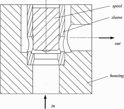
A typical structure of a cartridge valve is shown in Figure 1, which is also taken as the investigated subject for this paper. It is mainly composed of three parts: housing, sleeve and spool.

Figure 1. Structure of a cartridge valve.

Flow force and flow rate are significant factors in modeling a valve since they have great influence on the designing and controlling of the valve (Wang, Cai, Kawashima, & Kagawa, 2005). Typically, the two key parameters can be calculated by: (1) Where is the flow rate through the valve; stands for the steady flow force (transient flow force is usually neglected because it is relatively small) (Merritt, 1967). is the discharge coefficient; is the flow area of the valve which is a function of the displacement of the spool and jet angle . is the pressure drop through the valve, while is the static pressure of the inlet surface.

The above equation shows that or has a relatively simple and explicit relationship with and . However, the remaining parts of the equations induce some uncertainty and inaccuracy.

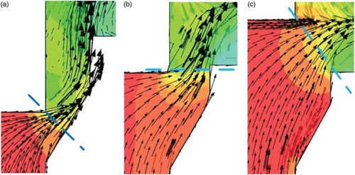
For example, flow area can be calculated only under certain simplifications and assumptions but can vary among several states in an actual situation (Amirante, Moscatelli, & Catalano, 2007). For cartridge valves, flow area is often calculated by assuming that flow cross-section area is the cone frustum from the edge of the spool to the poppet surface of the sleeve (like Figure 2(a)). But actually the position and shape of the cross-section area keep varying as the spool opening changes, as shown in Figure 2(b) and (c), which makes it hard to calculate accurately (Kong, 2015).

Figure 2. Variation of flow area and jet angle when spool opening changes; (a) cross-section location at spool opening 2 mm; (b) cross-section location at spool opening 5 mm; (c) cross-section location at spool opening 8 mm.

And as the flow area is hard to calculate, the discharge coefficient and the jet angle are far more elusive. In practical application, especially for cartridge valves which have a larger range for the displacement of the spool, a fixed value of or is usually not sufficient to manifest the feature of the flow through the flow area (Wu, Burton, & Schoenau, 2002).

Some efforts have been made to overcome this difficulty. Some implemented varying discharge coefficient number from experiment or simulation to make compensation (Knutson & Van de Ven, 2016; Valdés, Miana, Núnez, & Pütz, 2008; Viall & Zhang, 2000), and others used actual experiment data to derive a behavioral model to match the real performance of the valve better (Liu & Yao, 2006; Prescott & Ulanicki, 2003). These efforts were intended to find a better way to predict the variation of discharge coefficient or jet angle, but it seems to be a self-justifying procedure because the number of discharge coefficient is essentially calculated by a known flow rate and then it is used to recalculate the flow rate. Moreover, unlike traditional slide-spool valves, the fluid field geometry of cartridge valves varies significantly during the overall stroke of the spool, making it even more difficult to predict the value of discharge coefficient.

The CFD method is now taken as the popular way to study characteristics of hydraulic valves (Del Vescovo & Lippolis, 2006), and its accuracy has been validated by some experimental research (Amirante, Vescovo, & Lippolis, 2006; Simic & Herakovic, 2015). But few of these results from CFD research can be applied to the modeling of the valve or the hydraulic system because of the large amount of data involved and relatively inflexible boundary conditions.

Given the problems mentioned above, the purpose of this paper is to develop a method to describe the flow force and flow rate characteristics of the valve in the whole opening range while reducing the uncertainties involved and amount of data needed. 3D CFD flow field simulation with dynamic mesh technique was implemented to get the detailed characteristics of the valve flow field at different spool displacements. And POD was introduced to simplify the flow field data. By extracting the first few major modes of the transient flow field and using them to reconstruct the fluid field at a specific time, we can master the main data needed to specify the characteristics of the valve. In this way, we can calculate the force acting on the spool or flow rate through the valve directly from the flow field data, skipping the traditional calculation equations which bring uncertainty and inaccuracy.

3. 3D flow field simulation for cartridge valves

3.1 Steady flow field simulation

In order to prove the feasibility and reliability of 3D flow simulation in researching the valve characteristics, steady-state flow simulation was conducted at first. The fluid field was meshed with commercial software ICEM into unstructured tetrahedral mesh. Numerical simulation was carried out in commercial software FLUENT.

Boundary conditions were set according to the operating conditions of the valve. Inlet part was set to be velocity inlet, which defines the flow rate through the valve (as flow rate is determined by the pump in the experiment), and outlet was pressure outlet which defines the back pressure. Other surfaces were assumed to be rigid wall with no slip in steady-state simulation. Working medium was considered to be incompressible with a constant density 860 and dynamic viscosity 0.02 . Double-precision, pressure-based solvers were used, and model with standard wall function was selected for turbulence evaluation. As is required by turbulence theory, was valued at 50, and thus the first cell height can be calculated to be 0.4 mm to make sure the first layer cell be located in the core region. Residuals of for continuity, velocity and were used as the threshold of iteration convergence.

When the solution is converged, characteristics of the valve can be derived. Flow rate versus pressure drop of the valve can be obtained by checking the flow rate and area-weighted average pressure on the surface of inlet and outlet. And the value of the force acting on the spool with flow force is equal to the integral of static pressure on the bottom surface of the spool.

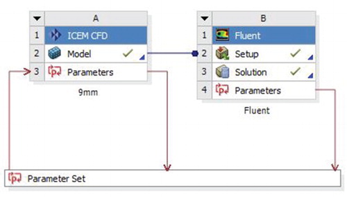
As mesh density and quality have significant influence on the simulation result and time consumption, mesh sensitivity analysis should be conducted to find a proper mesh size to trade-off between accuracy and computation effort. Workbench platform is used to conduct this work. An ICEM module is employed to change the global size of the mesh, and FLUENT is used to do the calculation afterwards (as shown in Figure 3).

Figure 3. Workbench diagram used in mesh sensibility research.

Other parameters set are kept all the same, and flow rate of the valve is used as the criterion to quantify simulation results. The global mesh size and corresponding flow rate and time consumption are shown in Figure 4.

Figure 4. Global mesh size and corresponding flow rate and time consumption.

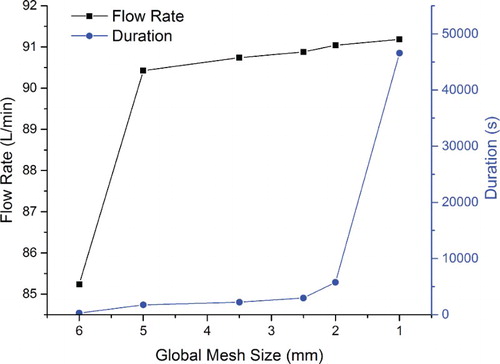
It can be seen that the simulated flow rate tends to converge slowly with an increasing mesh density while time consumption increases dramatically when mesh size reaches 1 mm. Considering both accuracy of simulation results and time consumption, global mesh size is chosen to be 2 mm.

3.2 Experimental validation of flow field simulation

In order to validate the correctness and accuracy of 3D CFD simulation, a fundamental experiment about the cartridge valve was carried out. The schematic of the test bench is shown in Figure 5.

Figure 5. Schematic of the experimental setup.

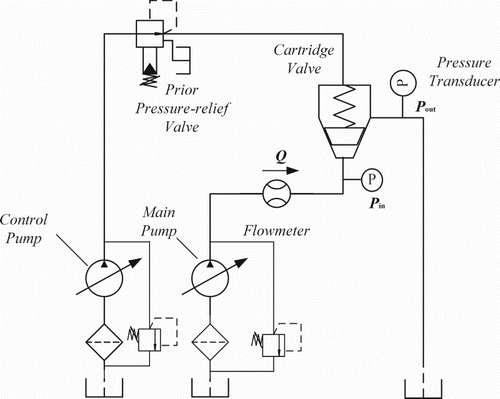
During the experiment, control pressure from the prior pressure-relief valve was set to 0 so that the spool can remain at the same displacement during the whole procedure. By regulating the flow rate of the main pump, flow rate through the cartridge valve and corresponding pressure at inlet and outlet can be measured and recorded. By plotting different pressure drop () versus the varying flow rate, the flow rate characteristic of the valve can be derived.

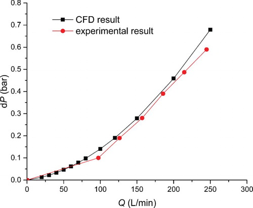
The flow rate characteristic resulting from CFD simulation as well as experiment is visualized in Figure 6. It can be seen that CFD simulation results agree well with that measured in the experiment, with a relative error within 7%. This demonstrates that 3D CFD simulation is an effective and reliable way to study the performance of the valve. And since the CFD method can provide rich and detailed information of the flow field of the valve, CFD results can be taken as the basis to study and model the valve.

Figure 6. Flow rate characteristic of the cartridge valve.

4. Modeling the valve by flow field decomposition and reconstruction

4.1 Basic concepts about POD

POD is a highly effectively method to cope with massive data and is widely used in processing fluid field information (Apacoglu, Paksoy, & Aradag, 2011). It describes a random, complex physical field by means of the sum of a series of basic functions (usually called mode or eigenmode). With these modes, we can capture the overwhelming majority of the original field (say, above 99%) with only the first several modes. This can significantly simplify the excessive amount of data in the origin flow field, so it is widely applied in the simplification of fluid mechanics (Selimefendigil, 2013).

The basic principle of the POD approach is to find an optimal set of orthogonal basis vectors on which the maximum projection of the vector space could be achieved (Ly & Tran, 1998). This can be mathematically defined as: (2) Where is the definition domain of the vector space; stands for inner product operation; is the 2-norm of a vector and is the fluctuation derived from the origin set by: (3) Eigenvalue and eigenvector methods (Hou, 2010) are most widely applied in solving the problem. The mathematical procedure can be expressed as: (4) Where is a matrix representing the correlation matrix of R. And is the k-th unitized eigenvector homologous with the eigenvalue of matrix : (5) Additionally, in order to weight the priority of the basis vectors, the eigenvalue of matrix C is often taken as the criterion (Keane & Nair, 2005). Cumulative proportion is often used to quantify the proportion of property captured by the first n basis: (6) According to existing definition (Volkwein, 2008), when the first l modes are used to reconstruct the original data, corresponding error can be calculated by: (7) Based on the above theory, the POD method can be utilized to simplify the original data of transient 3D CFD simulation results. The main property of the original fluid field can be captured, while the amount of data is significantly reduced. Using these decomposed data to model the characteristics of the cartridge valve can avoid the problems in the traditional modeling method mentioned in Section 1, thus the accuracy of the model can be improved.

4.2 Transient simulation with dynamic mesh technique

In the procedure of the POD method, a set of data representing the original field is needed first. A typical POD process is often used to handle the time-varying field such as the unsteady flow field around building surfaces (Tamura, Suganuma, Kikuchi, & Hibi, 1999). But in this case, what we are concerned about is the characteristics of the valve in relation with the displacement of the spool. So the spool displacement x is taken as the independent variable. Moreover, the origin data should be abundant enough to make sure that it contains necessary information of the valve characteristics.

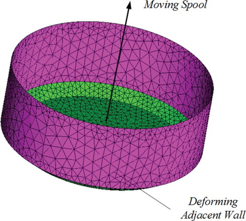
However, it would be very tedious work if we model and mesh the flow field at different spool displacements with tiny increment manually. So transient 3D CFD simulation with dynamic mesh technique was implemented to make this procedure easy. A constant velocity was exerted on the spool bottom surface by means of user-defined profiles, and the adjacent wall was set to be deforming when the spool surface moves upward and downward (as shown in Figure 7.). So the mesh of the whole fluid field can be smoothed and re-meshed to form the new computing zone.

Figure 7. Dynamic mesh setup.

The velocity of the spool was set to 1 , which is quite small in order to avoid the transient influence of the velocity of the spool. As previous study shows, although transient simulation with a velocity of the spool may cause a difference to the flow force, difference can be neglected when the velocity is relatively small (like smaller than 0.1 ) (Kong, Wei & Yan, 2016). In this case, steady-state simulation is run under the spool opening of three selected time step points, and the comparison of flow rate and spool force results showed little discrepancy (as shown in Table 1).

Table 1. Comparison of steady and transient simulation.

	Flow rate (kg/s)		Spool force (N)
Time step point	Steady simulation	Transient simulation	Steady simulation	Transient simulation
10	1.05	1.06	228.78	228.84
50	2.23	2.23	229.20	229.17
100	3.52	3.54	227.14	227.21

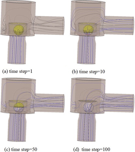
Time step was set to 0.1 s, and FLUENT automatically saves the data of the solution each time when the computation is converged. And in order to eliminate the influence of the direction of moving velocity further, a negative velocity was given to make the spool move reversely when the spool reaches maximum opening. So there are overall 200 time steps, and in this way we can harvest 200 sets of solution data covering the whole spool displacement range at intervals of 0.1 mm each. The variation of the fluid field geometry and flow streamline during the upward process is shown in Figure 8.

Figure 8. Variation of fluid field during transient simulation.

4.3 POD-based modeling of flow force and flow rate characteristics

Original data containing the flow field information at different spool displacement was obtained from transient CFD simulation with dynamic mesh. With these data the procedure of POD can be carried out as introduced in Section 4.1. Pressure field on the bottom of the spool was used to calculate the force acting on the spool and velocity field on outlet surface to calculate flow rate through the valve. The extracting of data and relevant calculation were done by MATLAB code according to mathematical basis in 4.1.

Using MATLAB code based on the mathematical theory of POD to process the pressure field on spool surface, we can get the decomposed flow field information. The distribution pattern of proportion and cumulative proportion for each mode are shown in Figure 9.

Figure 9. Proportion distribution pattern of each mode.

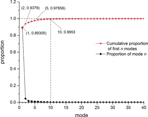
As shown in Figure 9, the eigenvalue of the first mode takes up 89.31% of the total proportion, which means the first mode captures a large majority of the information of the original field. And when the number of modes goes to 10, the percentage of cumulative proportion captured can be up to 99.53%, which means that the overwhelming majority of information of the fluid field is captured. So we select 10 modes to reconstruct the pressure field when modeling the force characteristics of the valve.

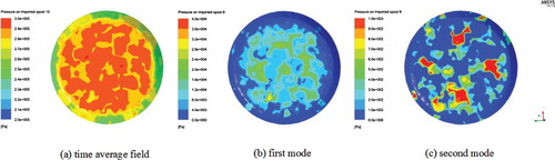
The pressure field on spool surface at spool displacement x = 4 mm is taken as an example of fluid field reconstruction (for the valve geometry is more like a traditional poppet valve at this opening). As the time-average value (Figure 10(a)) of all time step data is subtracted from original data set at first (Equation 3), the modes generated by POD represents the variance relative to the mean value. As is shown in Figure 10(b), the first mode represents the pressure decrease at the outer ring of the spool, which is the dominant reason causing flow force. The second mode also showed that there is pressure decrease near the center of the spool (Figure 10(c)), but the magnitude is smaller than the first mode. The third mode, as well as remaining modes, shows no specific pattern and the magnitude is small compared to the first two modes, so they are taken as time-varying disturbances.

Figure 10. Distribution pattern of the average value and first two modes.

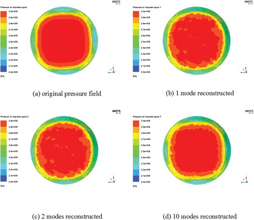
The fluid field can be reconstructed by adding up the first few modes to the average value. Figure 11 shows the original pressure field and that reconstructed with different modes of POD basis. As the proportion distribution in Figure 9 shows, the first mode reconstruction can capture a majority of the fluid field feature. And when the second mode is added, the reconstructed pressure field gets closer to the original one. With the growth of the number of modes used (which means more details are added), the reconstructed flow field becomes ever more identical with the original field.

Figure 11. Original and reconstructed pressure field.

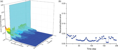
Reconstruction error defined in Equation (7) between the reconstructed pressure field modes and the original field is shown in Figure 12. It can be seen that as the number of modes used increases, the error between the reconstructed and the original field drops sharply. And when 10 modes are employed, reconstruction error can be kept under 5%.

Figure 12. Error between reconstructed and original field. (a) Reconstruction error under different modes and spool displacement; (b) Error of 10 modes reconstruction.

One problem remaining in calculating the flow force is that the simulation is undertaken under a certain inlet pressure. But unlike the flow rate which is only sensitive to pressure drop , the force is in direct correlation with the magnitude of pressure P, which may cause repetitive work to simulate under various pressure conditions. So here we employ the concept of flow force coefficient. As Equation (1) indicates, the steady-state flow force can be calculated by: (8) So the force exerted on the spool is: (9) Where is defined to be the flow force coefficient.

On the other hand, the force can also be calculated by directly integrating the pressure throughout the bottom surface of the spool: (10) By comparing Equations (9) and (10), we can find that for a single infinitesimal unit on the spool surface, the flow force coefficient can be expressed by: (11) Where is the distributing pressure on the spool surface, and is the inlet pressure. In this way the flow force coefficient can be calculated from the original simulation results. And when is taken as the variable to be processed by POD procedure, the value of inlet pressure no longer has influence on the distribution pattern of the pressure field on the spool, which brings great practical significance in modeling the valve.

For this valve specifically, there is a chamfer surface at the end of the spool (which can be seen in Figure 1). As the force calculated here is just in the vertical direction, the force on the chamfer should be multiplied with the cosine of the chamfer angle. So the spool is actually divided into two zones, and the flow force coefficient k is calculated respectively as k₁ and k₂, hence the force is calculated by: (12) Where and stand for the flow force coefficient of each unit on surface 1 and surface 2 and is the angle of the chamfer.

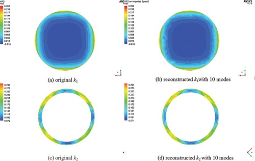
By taking flow force coefficient as the distributed parameter of the fluid field, we can implement the same process of decomposition and reconstruction like the pressure field. Figure 13 shows the original and reconstructed field of flow force coefficient on two parts of the spool. It can be seen that 10 modes are adequate to capture and reconstruct most information of the original field.

Figure 13. Original and reconstructed field of k on spool surface.

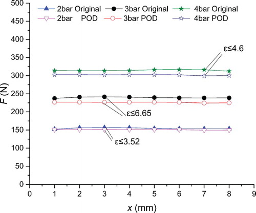
With the reconstructed field of k₁ and k₂, total force acting on the spool can be calculated by Equation (12). Figure 14 shows the calculation results of using the reconstructed field of flow force coefficient k under different inlet pressure. It can be seen that the force calculated by the POD method agrees with CFD results well and, since the flow force coefficient k is introduced, modes generated by one specific inlet pressure can also predict other inlet pressure conditions well.

Figure 14. CFD and POD results of F under different pressure and displacement.

Similarly, flow rate through the valve can be calculated by decomposing and reconstructing the velocity field on outlet surface. If the velocity field on outlet surface is known at a specific time, volume flow rate through the valve can be calculated by: (13) Where and are the area and normal velocity (y direction) of the number i grid on the outlet surface, which can be extracted from the solution data files.

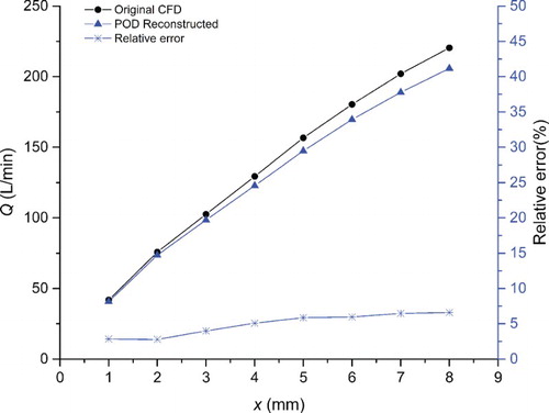
A similar procedure is used in the decomposition and reconstruction of velocity field, and the result is similar to the previous one. With the reconstructed velocity field, flow rate through the valve can be calculated by Equation (13) using corresponding MATLAB code. Figure 15 shows the flow rate and relative error calculated by CFD and POD method. It can be seen that POD-reconstructed velocity field can help to predict the flow rate of the valve with satisfactory accuracy.

Figure 15. Flow rate and relative error calculated by the reconstructed velocity field.

The above procedure is carried out for the case of a single pressure drop . Although the flow rate characteristic does have some relationship with Reynolds number, in most cases the fluid through a valve is turbulent so the influence of Reynolds number is neglected (Wu et al., 2002) and the flow rate under a given spool displacement is now considered to be only related to the pressure drop. In consideration of the quadratic relationship between flow rate Q and pressure drop (as specified in Equation (1)), the flow rate under other pressure drops can be calculated easily by multiplying a scaling coefficient .

In order to verify this deduction, CFD simulation was carried out under other pressure drop, and corresponding flow rate was calculated. The comparison of results generated from the two methods is shown in Figure 16.

Figure 16. CFD and POD results of Q under different pressure drop.

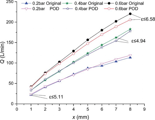
The results showed that by multiplying a scaling coefficient the flow rate calculated through POD method can predict the flow rate for other pressure drop conditions quite well. This ensures that the POD method can model the characteristics of the valve under various conditions and can be implemented in practical modeling applications.

5. Application of POD results in modeling a cartridge valve

The method of POD decomposition and reconstruction has been proved to be effective in predicting the flow rate and flow force characteristics of a cartridge valve while avoiding uncertainty and inaccuracy in traditional modeling formula. So in this part we implement the result of POD in modeling a cartridge valve and compare it with the model constructed with traditional module. The model is constructed in the widely used hydraulic modeling platform AMEsim.

Figure 17(a) shows the cartridge valve model constructed using existing submodule BAP28, which represents the one-dimensional motion of a double cone poppet valve with a conical seat (Imagine, 2004). The value of flow coefficient is tuned according to the flow rate at spool displacement x = 4 mm, and other parameters such as spool diameter and poppet angle are set according to the geometry model. Figure 17(b) is constructed by applying the results of POD method which calculates the coefficient of flow rate and flow force from the POD file using MATLAB code.

Figure 17. Valve model created with two methods: (a) valve model using traditional component; (b) valve model using POD results.

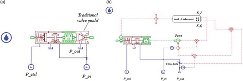
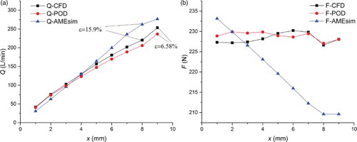
Figure 18 shows the results of the two models when spool displacement varies from 1 to 9 mm. It can be seen that relative error between the flow rate calculated by the AMEsim model and that with CFD simulation can be up to 15.9%, while the maximum relative error for the POD model is 6.58%. For flow force characteristics, force calculated by the POD model agrees well with the CFD result, but the one calculated by traditional model has a greater difference both in values and trends. This is because the fixed coefficients are difficult to adapt to the changes of the valve shape throughout whole valve opening in actual work process.

Figure 18. Simulation results of CFD, POD method and traditional model: (a) flow rate at different spool opening; (b) spool force at different spool opening.

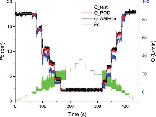
In order to verify the results of this work, an experiment is conducted using the test system shown in Figure 5. Control current from 0 to 300 mA (maximum) and then back to 0 with an increment of 25 mA is given to the prior pressure-relief valve so that the output control pressure changes correspondingly (the green line in Figure 19). The flow rate through the valve decreases from the system flow rate to zero and rises back again (as represented by the black line). The same control pressure curve is used as input in the two AMEsim models in Figure 17. Flow rate responses of the two models are presented by the red line (model created with POD results) and blue line (model created with traditional AMEsim submodel). It can be seen that the response of the model created with POD results is in better agreement with experimental data, which means the application of POD results helps in improving the accuracy in modeling the cartridge valve since it avoids uncertain coefficients in traditional formula.

Figure 19. Flow rate response of two models and experimental data.

6. Conclusion

In this paper, the POD method is employed in modeling key characteristics of a cartridge valve. Velocity field on the outlet surface is processed to model flow rate, and flow force coefficient representing pressure field on spool surface is used to calculate the spool force with flow force influence.

By using few modes to reconstruct the field we can calculate flow rate and spool force with satisfactory accuracy and simplified data. Also, flow force coefficient was introduced and processed with the POD method to make sure that this method is not confined to the working states which has been simulated by CFD, but can predict flow force under other input pressure conditions as well.

Simulation results showed that the response of the model employing POD results agrees better with CFD results as well as actual response in experiments than traditional model. Accuracy of flow rate and spool force prediction are improved since the use of uncertain parameters such as discharge coefficient and jet angle is avoided. This means the application of the POD method can be helpful in the modeling and studying of hydraulic valves in engineering applications.

Disclosure statement

No potential conflict of interest was reported by the authors.

Additional information

Funding

This work was supported by the National Natural Science Foundation of China (NSFC) [grant number 51475041].

References

- Amirante, R., Moscatelli, P. G., & Catalano, L. A. (2007). Evaluation of the flow forces on a direct (single stage) proportional valve by means of a computational fluid dynamic analysis. Energy Conversion and Management, 48(3), 942–953. DOI:doi: 10.1016/j.enconman.2006.08.024
- Amirante, R., Vescovo, G. D., & Lippolis, A. (2006). Flow forces analysis of an open center hydraulic directional control valve sliding spool. Energy Conversion and Management, 47(1), 114–131. DOI:doi: 10.1016/j.enconman.2005.03.010
- Apacoglu, B., Paksoy, A., & Aradag, S. (2011). CFD analysis and reduced order modeling of uncontrolled and controlled laminar flow over a circular cylinder. Engineering Applications of Computational Fluid Mechanics, 5(1), 67–82. DOI:doi: 10.1080/19942060.2011.11015353
- Chalet, D., & Chesse, P. (2010). Analysis of unsteady flow through a throttle valve using CFD. Engineering Applications of Computational Fluid Mechanics, 4(3), 387–395. DOI:doi: 10.1080/19942060.2010.11015326
- Del Vescovo, G. D., & Lippolis, A. (2006). A review analysis of unsteady forces in hydraulic valves. International Journal of Fluid Power, 7(3), 29–39. doi: 10.1080/14399776.2006.10781256
- Fu, L., Wei, J., & Qiu, M. (2008). Dynamic characteristics of large flow rating electro-hydraulic proportional cartridge valve. Chinese Journal of Mechanical Engineering, 21(6), 1. DOI:doi: 10.3901/CJME.2008.06.057
- Hou, Y. (2010). Reduced-order modeling of incompressible jet flow using proper orthogonal decomposition and Galerkin projection (Doctoral dissertation). Retrived from ProQuest Dissertations Publishing. (2010.1489254.)
- Imagine, S. A. (2004). AMESim (Version 4.2) [computer software]. Roanne, France: Imagine.Lab.
- Jelali, M., & Kroll, A. (2003). Hydraulic servo-systems: Modelling, identification and control. London: Springer Science & Business Media.
- Keane, A., & Nair, P. (2005). Computational approaches for aerospace design: The pursuit of excellence. Hoboken: John Wiley & Sons.
- Knutson, A. L., & Van de Ven, J. D. (2016). Modelling and experimental validation of the displacement of a check valve in a hydraulic piston pump. International Journal of Fluid Power, 17(2), 114–124. DOI:doi: 10.1080/14399776.2016.1160718
- Kong, L. (2015). Research of the characteristics and control method of oil-charging and discharging cartridge valves for hydrodynamic retarders (Master’s thesis). Retrieved from CDMD.CNKI. (U463.5.2015)
- Kong, L., Wei, W., & Yan, Q. (2016, November). Flow force analysis of cartridge valve with conical seat based on 3D flow field simulation. Paper presented at the meeting of The Ninth Fluid Power Transmission and Control Conference of China, Hangzhou, China.
- Liu, S., & Yao, B. (2006). Automated onboard modeling of cartridge valve flow mapping. IEEE/ASME Transactions on Mechatronics, 11(4), 381–388. doi: 10.1109/TMECH.2006.878552
- Ly, H. V., & Tran, H. T. (1998). Proper orthogonal decomposition for flow calculations and optimal control in a horizontal CVD reactor. Quarterly of Applied Mathematics, 631–656. DOI:doi: 10.1090/qam/1939004
- Merritt, H. E. (1967). Hydraulic control systems. Hoboken: John Wiley & Sons.
- Prescott, S. L., & Ulanicki, B. (2003). Dynamic modeling of pressure reducing valves. Journal of Hydraulic Engineering, 129(10), 804–812. DOI: 10.1061/(ASCE)0733-9429(2003)129:10(804 doi: 10.1061/(ASCE)0733-9429(2003)129:10(804)
- Selimefendigil, F. (2013). Numerical analysis and pod based interpolation of mixed convection heat transfer in horizontal channel with cavity heated from below. Engineering Applications of Computational Fluid Mechanics, 7(2), 261–271. DOI:doi: 10.1080/19942060.2013.11015469
- Simic, M., & Herakovic, N. (2015). Reduction of the flow forces in a small hydraulic seat valve as alternative approach to improve the valve characteristics. Energy Conversion and Management, 89, 708–718. doi: 10.1016/j.enconman.2014.10.037
- Tamura, Y., Suganuma, S., Kikuchi, H., & Hibi, K. (1999). Proper orthogonal decomposition of random wind pressure field. Journal of Fluids & Structures, 13(7), 1069–1095. DOI:doi: 10.1006/jfls.1999.0242
- Valdés, J. R., Miana, M. J., Núnez, J. L., & Pütz, T. (2008). Reduced order model for estimation of fluid flow and flow forces in hydraulic proportional valves. Energy Conversion and Management, 49(6), 1517–1529. DOI:doi: 10.1016/j.enconman.2007.12.010
- Viall, E. N., & Zhang, Q. (2000). Determining the discharge coefficient of a spool valve. In American control conference, 2000. Proceedings of the 2000 (Vol. 5, pp. 3600–3604). IEEE. DOI:doi: 10.1109/ACC.2000.879241
- Volkwein, S. (2008). Model reduction using proper orthogonal decomposition. Lecture Notes, Institute of Mathematics and Scientific Computing, University of Graz. Retrieved from http://www.uni-graz.at/imawww/volkwein/POD.pdf
- Walters, R. B. (2000). Hydraulic and electric-hydraulic control systems. Dordrecht: Kluwer academic publishers.
- Wang, T., Cai, M., Kawashima, K., & Kagawa, T. (2005). Modelling of a nozzle-flapper type pneumatic servo valve including the influence of flow force. International Journal of Fluid Power, 6(3), 33–43. doi: 10.1080/14399776.2005.10781228
- Wasewar, K. L., & Sarathi, J. V. (2008). CFD modelling and simulation of jet mixed tanks. Engineering Applications of Computational Fluid Mechanics, 2(2), 155–171. DOI:doi: 10.1080/19942060.2008.11015218
- Wu, D., Burton, R., & Schoenau, G. (2002). An empirical discharge coefficient model for orifice flow. International Journal of Fluid Power, 3(3), 13–19. doi: 10.1080/14399776.2002.10781143