Predictions of ship maneuverability based on virtual captive model tests

Abstract

Maneuverability is an important hydrodynamic performance of a ship, and should be taken into account during the ship design stage. The present study of Computational Fluid Dynamic (CFD) calculations aims to offer a numerical tool for maneuvering prediction with high accuracy. The virtual captive model tests for a model scale KCS container ship are conducted using unsteady Reynolds-averaged Navier–Stokes (RANS) computation to obtain the full set of linear and nonlinear hydrodynamic derivatives in the 3rd-order Abkowitz model. The numerical uncertainty analysis is carried out for the pure sway and yaw–drift tests to verify the numerical accuracy. It is concluded that the lower order Fourier coefficients are preferred in the computation of the hydrodynamic derivatives. Moreover, part of the computed hydrodynamic forces and moments are compared with the available captive model test data, and good agreement is obtained. By substituting the computed hydrodynamic derivatives into the mathematical model, the standard turning and zigzag maneuvers are predicted. By comparing the predicted maneuvering results with the available experimental data and the prediction results by others, it is demonstrated that acceptable prediction accuracy can be achieved with the present method, which shows the effectiveness of the present method in predicting ship maneuverability.

KEYWORDS:

• Maneuverability prediction
• Abkowitz model
• hydrodynamic derivatives
• RANS
• virtual captive model tests

1. Introduction

Maneuverability is an important hydrodynamic performance of a ship. The International Maritime Organization (IMO) has promulgated the Standards for Ship Manoeuvrability (IMO, 2002) to ensure the safety of navigation. To assess ship maneuverability at the design stage, reliable methods for predicting ship maneuverability are required. The Manoeuvring Committee of the International Towing Tank Conference (ITTC, 2008) and the Workshop on Verification and Validation of Ship Manoeuvring Simulation Methods (SIMMAN, 2008, 2014) collected and sorted all methods for prediction of ship maneuverability in practical applications. In general, maneuverability predictions using free running model tests (FRMT) such as zigzag and turning circle tests are believed to be most close to the reality. At the SIMMAN workshops, many organizations such as Maritime Research Institute Netherlands (MARIN) provided FRMT data for the standard ship models KVLCC1 & 2, KCS and DTMB 5415 (Quadvlieg, 2017). Besides, the system-based prediction method, which uses the mathematical model of maneuvering motion with the hydrodynamic coefficients obtained from empirical formulae (EMP) (Kijima, Katsuno, Nakiri, & Furukawa, 1990), captive model tests, numerical computations, or system identifications (Sutulo & Guedes Soares, 2014; Tran Khanh, Ouahsine, Naceur, & El Wassifi, 2013; Zhang & Zou, 2011), is widely applied. Among the methods for determining the hydrodynamic coefficients, the captive model test method is regarded as the most reliable one, which includes an oblique towing test, rudder force test, planar motion mechanism (PMM) test, and circular motion test (CMT), etc. The advantage of the captive model test is that it can obtain all the linear and nonlinear hydrodynamic coefficients in the mathematical model. However, it also has some drawbacks, such as the fact that specific test facilities are required, and it is not convenient for the evaluation and optimization of ship maneuverability at the design stage.

Nowadays, with the rapid development of computer techniques and the Computational Fluid Dynamics (CFD) method, CFD-based numerical methods have been successfully applied in the naval architecture (Zhang, Zhang, Tezdogan, Xu, & Lai, 2018), especially in the investigation of ship maneuverability (Stern, Yang, Wang, Sadat-Hosseini, & Mousaviraad, 2013; Sun, Su, Wang, & Hu, 2016). There are two types of CFD application in maneuvering predictions. One is the direct numerical simulation of standard maneuvers in the full time domain with steering rudder(s) and rotating propeller(s) (Dubbioso, Durante, Di Mascio, & Broglia, 2016; Wang, Zou, & Wan, 2017). However, the requirement of huge computational resources and the heavy computational burden limit its practical application. Another CFD application is more practical. It first determines the maneuvering hydrodynamic forces by conducting virtual captive model tests, i.e. simulating the captive model tests with a Reynolds-averaged Navier–Stokes (RANS)-based solver, and then predicts the standard maneuvers using the mathematical models with the obtained hydrodynamic coefficients. Two classic types of mathematical models – the Abkowitz model (Abkowitz, 1964) and the Maneuvering Modeling Group (MMG) model (Yasukawa & Yoshimura, 2015) – for predicting ship maneuverability are generally adopted. More and more researchers are trying to use CFD methods for predicting the hydrodynamic derivatives. Otzen and Simonsen (2014) and Simonsen, Otzen, Klimt, Larsen, and Stern (2012), identified a reduced test matrix to be applied for PMM simulations, and standard maneuvers were conducted for the appended KCS ship model by using the Abkowitz model. Sakamoto, Carrica, and Stern (2012) conducted unsteady RANS (URANS) simulations of static and dynamic PMM tests for an un-appended surface combatant model 5415. Sung, Park, and Jun (2015) developed an easy procedure of virtual captive model tests to obtain the linear and nonlinear hydrodynamic derivatives for un-appended KCS and KVLCC1 & 2. He et al. (2016) computed the linear hydrodynamic derivatives of the KVLCC2 ship model by numerically simulating pure sway and pure yaw tests and performed the standard free running maneuvers using MMG mathematical model. Jin, Duffy, Chai, Chin, and Bose (2016) investigated the influence of scale effects on maneuvering coefficients for a KVLCC2 hull by using a URANS solver. Veedu and Krishnankutty (2016) investigated the effect of vessel speed on the hydrodynamic derivatives of the container ship S175. Shenoi, Krishnankutty, and Selvam (2016) numerically studied the maneuvering qualities of S175 using the derivatives obtained by a RANS-based solver, with the nonlinear and roll-coupled effects being taken into account. Liu, Zou, and Zou (2017) analyzed the effect of dynamic sinkage and trim on the hydrodynamic forces and hydrodynamic derivatives by numerically simulating static captive model tests. Guo and Zou (2017) conducted a system-based investigation on four degrees of freedom (4-DOF) ship maneuvering in calm water for the ONR tumblehome model by RANS simulation of captive model tests. A similar study for a destroyer hull was presented in Alexandersson, Korkmaz, and Mazza (2017).

The virtual captive model tests have become a robust tool for acquiring the hydrodynamic derivatives/coefficients in the mathematical model of maneuvering motion at ship design phase. But few get the full set of the hydrodynamic derivatives/coefficients by this method. Most researchers used a modular model such as the MMG model in which the hull–rudder–propeller interaction coefficients were obtained by empirical formulae (He et al., 2016; Shenoi et al., 2016) or model tests (Sung et al., 2015). Others using the Abkowitz model simplified the mathematical model (Otzen & Simonsen, 2014; Simonsen et al., 2012). So far, no full set of hydrodynamic derivatives in the Abkowitz model has been presented for the KCS container ship. Most recently, Quadvlieg (2017) pointed out that the comparisons among numerical results from different institutes for the KCS ship under the same maneuvering conditions were not satisfactory. There was too much scatter in the predicted maneuvering parameters. To verify the reliability of CFD-based tools in maneuvering predictions better, more numerical simulations are needed to expand the database. Under this background, the present study aims to predict KCS ship’s maneuverability using the Abkowitz model with the full set of linear and nonlinear hydrodynamic derivatives all determined by virtual captive model tests. The Abkowitz model is preferred since the effects of the hull–rudder–propeller interactions are automatically included and there is no need to determine the hull–rudder–propeller interaction coefficients. The paper is organized as follows. Firstly, grid and time-step dependency studies are carried out for a pure sway case and a yaw–drift case to estimate the numerical error and uncertainty due to grid discretization and time step. Then systematic computations are performed, and the predicted hydrodynamic forces and moments are presented and discussed. Some of the predicted forces and moments are compared with the available experimental data for validation purposes. Finally, by using the hydrodynamic derivatives determined from the virtual captive model tests, simulations of standard maneuvers are carried out and the results are compared with FRMT and CFD-based prediction results in the literature to validate the present numerical method and the established mathematical model.

2. Mathematical model

2.1. Coordinate systems

Two right-handed coordinate systems are adopted, as shown in Figure 1. The body-fixed coordinate system o-xyz is used for computing the hydrodynamic forces. Its x-axis is pointing to the bow, y-axis pointing to starboard. The origin locates at the intersection of the water-line plane and the center-line plane at the mid-ship section. It is also the captive point in the captive model tests. The earth-fixed coordinate system o₀-x₀y₀z₀ is set up to define the ship motion. The o₀-x₀y₀ plane is fixed on the undisturbed free surface and the z₀-axis is pointing vertically downwards. u, v, and r are the surge velocity, sway velocity, and yaw rate in the body-fixed coordinate system; ψ is the heading angle (=r). X and Y are the external force components in the longitudinal and transverse directions, respectively; N is the external moment about the ship’s vertical axis. β is the drift angle defined by β=tan^–1(–v/u); δ is the rudder angle defined as positive when it turns to the port. U is the ship speed defined as .

Figure 1. Coordinate systems and variables.

2.2. The Abkowitz model

The Abkowitz model for maneuvering motion in 3-DOF, i.e. surge, sway, and yaw is: (1) where m is the ship mass, x_G is the longitudinal position of ship’s gravity center in the body-fixed coordinate system. I_z is the moment of inertia about the z-axis. , and are the corresponding surge acceleration, sway acceleration, and yaw acceleration. Strøm-Tejsen and Chislett (1966) provides a full set of the expansion equations for the hydrodynamic forces and moment with detailed hydrodynamic derivations: (2) (3) (4) where is the disturbance in surge velocity. u₀ is the surge velocity in the initial state of forward motion. , , , etc. are called hydrodynamic derivatives.

2.3. Captive model tests

There are two modes of captive model tests, ‘static’ and ‘dynamic’. In the static mode, the model is constrained to move with a constant captive speed. Typical static captive model tests include a static drift test with a given drift angle β, a static rudder test with a given rudder angle δ, and a rudder–drift combined test with a given drift angle β and a given rudder angle δ. A static drift test is used to determine the derivatives relative to v (,,,,,,,). Similarly, the hydrodynamic derivatives relative to δ (,,,,) and the cross-coupled derivatives relative to v and δ (,,,,) can be determined from the static rudder test and the rudder–drift combined test, respectively. In these static tests, the captive speed is =U.

In the dynamic mode, typically the PMM tests, the model is forced to oscillate in a sinusoidal way so that various combinations of sway and yaw motions are achieved, including pure sway test, pure yaw test, yaw–drift, and yaw–rudder combined tests. In the present study, the pure sway test is used to determine the acceleration derivatives (,) with v oscillating harmonically (, where the subscripts ‘max’ denote the amplitude, ω is the angular frequency), while the pure yaw test is used to determine the derivatives relative to the yaw rate, r (,,,,,,) with harmonic oscillating yaw motion (, , ). The yaw–drift combined test is used to determine the cross-coupled derivatives (,,,,) with r oscillating harmonically and a prescribed drift angle β superposed (, ), while the yaw–rudder combined test is used to determine the cross-coupled derivatives (,,,,) with r oscillating harmonically (, , ) and a prescribed rudder angle δ superposed. In the dynamic tests, for <<1.

2.4. Computation of the hydrodynamic derivatives

For the static captive model tests, Equations (2)–(4) can be simplified as follows:

Static drift: (5) Static rudder: (6)

Rudder–drift: (7)

The hydrodynamic derivatives in Equations (5)–(7) can be obtained as polynomial coefficients by the least-square curve fitting method when the hydrodynamic forces and moments X, Y, N on the ship model have been acquired.

A pure sway test is mainly conducted to determine the linear acceleration derivatives (,) by imposing dynamically varying v and . For the pure sway test, Equations (2)–(4) can be simplified as: (8) For other dynamic captive model tests, the simplified mathematical models similar to Equation (8) can be obtained.

For the dynamic captive model tests, the Fourier series (FS) method (Sakamoto et al., 2012) is adopted for deriving the hydrodynamic derivatives from the hydrodynamic forces and moment X, Y, N. Since the sway and yaw motions are prescribed by sine and cosine functions, the forces and moment can be reconstructed as a Fourier series with the angular frequency ω of sway/yaw motion: (9) where f (here X, Y, N) represents the time series of forces and moment; f_cn and f_sn are the nth-order Fourier sine and cosine coefficients, respectively.

On the other hand, for a pure sway test, the harmonic forms determined by substituting the model motion equation (, ) into the simplified mathematical model Equation (8) are: (10)

By using the same method, expressions similar to Equation (10) for other dynamic captive model tests can also be obtained. The Fourier sine and cosine coefficients in these expressions are given in Table 1. The functions of the N component are not listed in the table since they are the same as those of the Y component, and can be obtained by replacing ‘Y’ with ‘N’. For the same reason, the functions in the yaw–rudder test are not listed in the table since they can be obtained by replacing ‘v’ in the functions of the yaw–drift test with ‘δ’.

Table 1. Mathematical models for dynamic mode.

	X component	Y component
Pure sway
Pure yaw
Yaw–drift

Note: * MRL method

The ‘Multiple-Run (MR)’ approach (Yoon et al., 2015) is used to evaluate the hydrodynamic derivatives from these FS coefficients. This method uses curve-fittings of the mathematical models for sine and cosine coefficients similarly with the method for evaluating the derivatives of static captive tests mentioned above. The dynamic captive model tests are repeated over a range of test parameters of interest (e.g. v_max for pure sway or r_max for pure yaw test) to construct polynomial functions that best fit to the series of coefficients X₀, Y₀, N₀, X_sn, Y_sn, N_sn, X_cn, Y_cn, N_cn. For example, a cubic function (see Table 1) for pure yaw motion is curve-fitted to the 1st-order Fourier sine coefficient Y_s1 obtained from a series of pure yaw (varied r_max) tests to determine and . While all derivatives are available from the 0th- or the 1st-order coefficients, a few derivatives are also available from the higher order (the 2nd- or the 3rd-order) coefficients. The former is named as the MRL method (marked with an asterisk in Table 1) and the latter as the MRH method (Yoon et al., 2015).

The surge derivatives such as ,, and in Equations (2)–(4) are determined by repeating the straight ahead case for a range of the captive speed with the constant propeller revolutions (Strøm-Tejsen & Chislett, 1966). The longitudinal force X, which represents the difference between the propeller thrust and the ship resistance, will vary as a function of speed u. From Equation (2) it follows that: (11) The hydrodynamic derivatives , , can be obtained directly as the coefficients of the 3rd-order polynomial. Derivatives such as ,,,,,,,,,,,,evaluated at may also change with and can be expressed as appropriate polynomial functions f(u) similar to Equation (11) by repeating the static drift test, static rudder test, rudder–drift test, pure yaw test, yaw–drift test, and yaw–rudder test at different surge speeds, respectively. With the computed hydrodynamic derivatives so defined, Equation (1) is numerically solved using Euler’s difference method (Obreja, Nabergoj, Crudu, & Păcuraru-Popoiu, 2010) to simulate the standard maneuvers.

It should be noted that all governing equations are made non-dimensional by the speed , ship length L_pp, and water density ρ. This provides the following non-dimensional forms: (12)

Since all the variables in Equation (12) are non-dimensional, the resultant hydrodynamic derivatives are non-dimensional as well.

3. Numerical method

To numerically simulate the captive model tests, the CFD software STAR-CCM+ (CD-Adapco, 2014) is applied. The code solves an incompressible unsteady RANS equation, closed by modeling the Reynolds stress tensor using the Realizable k–ϵ turbulence model (Shih, Liou, Shabbir, Yang, & Zhu, 1995). The reason to choose the Realizable k–ϵ model is that this model has been extensively used for predicting the hydrodynamic forces on a maneuvering ship. As noted by Quérard, Temarel, and Turnock (2008), the k–ϵ model for prediction of the hydrodynamic coefficients of ships is quite economical in terms of CPU time, compared to, for example, the SST turbulence model, which increases the required CPU time by nearly 25%.

The VOF method (Hirt & Nichols, 1981) is applied to capture the position of the free surface. A SIMPLE algorithm (Patankar & Spalding, 1972) is employed for pressure–velocity coupling. A finite volume method (FVM) is used to discretize the flow domain into a finite number of control volumes (CVs) corresponding to computational grid cells. The temporal discretization is based on a 1st-order Euler difference, and the spatial discretization is performed with a 2nd-order upwind scheme for the convection term and secondary gradient contribution for the diffusion term. Mean flow quantities near the wall are simulated according to an all-y+ wall treatment where blended wall function is adopted (CD-Adapco, 2014). The all-y+ wall treatment is a hybrid treatment that attempts to emulate the high-y+ wall treatment for coarse meshes, and the low-y+ wall treatment for fine meshes. It is also formulated with the desirable characteristic of producing reasonable solutions when the wall–cell centroid falls within the buffer region of the boundary layer. Particularly, ship speed and drift angle are specified with the Dynamic Fluid Body Interaction (DFBI) Translation and Rotation module. It involves actual displacement of mesh vertices, which can model the 6-DOF motion of rigid body within the fluid system. Then the resultant force and moment acting on the body due to all influences are calculated, and the flow field is updated to find the new position and orientation of the ship. More details about the DFBI formulation can be found in Ohmori (1998).

The studies by Yao (2015) and Zipfel, Wagner, and Abdel-Maksoud (2014) showed that comparing the full propeller model by RANS simulation with a propeller body force model based on the actuator disk concept (Stern, Kim, Patel, & Chen, 1988), a fair overall agreement for the predicted total force can be achieved. Therefore, in the present study the rotating propeller is modeled as the body force radially distributed in the propeller disk with axial and tangential components. The body force is specified in a non-iterative manner in which the ship wake on the body force is neglected. The lateral force due to the propeller is ignored in the present study under the assumption that the propeller lateral force is a very small part of the total transverse force.

4. Numerical computation

4.1. Ship model

The ship form studied in this paper is the KCS container ship model with bulbous bow and transom stern, appended with a suspended rudder and a propeller. The designed approaching speed is 24 knots in full scale. It is one of the benchmark ships used at SIMMAN for CFD validation analysis. The 1/52.667 scaled ship model with a length between perpendiculars of L_pp=4.3671 m and draught d = 0.20506 m is chosen. The particular dimensions are listed in Table 2. More details of the geometrical properties can be found in the SIMMAN (2014) website.

Table 2. Main particulars of KCS.

Main particulars	Full scale	Model scale
Hull
Length between perpendiculars Lpp(m)	230	4.3671
Breadth B (m)	32.2	0.6114
Draught d (m)	10.8	0.20506
Displacement volume ∇ (m^3)	52,030	0.3562
Block coefficient CB (-)	0.651	0.651
Midship section coefficient CM (-)	0.985	0.985
Longitudinal center of gravity LCG (m)	111.6	2.119
Yaw radius of gyration kzz /Lpp (-)	0.25	0.25
Rudder
Rudder area SR (m^2)	115	0.0415
Lateral area of rudder AR(m^2)	54.45	0.0196
Propeller
Diameter D (m)	7.90	0.15
Propeller center, long. location (from FP) xp/Lpp(-)	0.9825	0.9825
Propeller center, vert. location (from keel) zp/Lpp (-)	0.02913	0.02913

4.2. Computation cases

In order to obtain the full set of linear and nonlinear hydrodynamic derivatives in the 3rd-order Abkowitz model (Equations (2)–(4)), a series of captive model tests are numerically simulated with the propeller operating at the ship propulsion point (14 rps). Details about the computational conditions are listed in Tables 3 and 4. These computational conditions are chosen according to the test setting (Simonsen, 2014) for a direct comparison with the test results. The two dynamic captive model cases marked with an asterisk in Table 4 are used for uncertainty analysis. The Froude number is defined as Fr=, where g is the gravitational acceleration. The calculations are carried out with the ship model fixed on even keel for static mode, while free to sink and trim for dynamic mode. The frequency f=ω/2π in the dynamic captive model tests is kept constant and equal to 0.075 s⁻¹ during all simulations, except one pure yaw case with 0.07667 s⁻¹ at Fr = 0.156. These simulations are run on two DELL local workstations each with 72 processors at 2.32 GHz.

Table 3. Computation cases for the static captive model tests.

Tests	Fr	β (°)	δ (°)
Static drift	0.26	0, ±0.5, ±1, ±2, ±4, ±8	0
	0.201	0, ±2, ±4, ±8, ±12	0
	0.156	0, ±4, ±8, ±12, ±16, ±20	0
Static rudder	0.26, 0.201, 0.156	0	0, ±10, ±20, ±25, ±30, ±35
Rudder–drift	0.26	±4, ±8	±10, ±20
	0.201	±4	0, ±10, ±20, ±25, ±30, ±35
		12	10, 20, 30, 35
	0.156	20	10, 20, 30, 35
		±12	0, ±10, ±20, ±25, ±30, ±35

Table 4. Computation cases for the dynamic captive model tests.

	Fr	β (°)	δ (°)	v'max	r'max
Pure sway	0.26	0	0	0.035, 0.07, 0.139, 0.206^a	0
	0.201	0	0	0.07, 0.139, 0.206, 0.139	0
Pure yaw	0.26	0	0	0	0.051, 0.101, 0.152, 0.202
	0.201	0	0	0	0.6, 0.406, 0.3, 0.2
	0.156	0	0	0	0.8, 0.611, 0.4, 0.2
Yaw–drift	0.26	±8, ±12, ±16, ±20	0	0	0.202
	0.201	+8^a, −8, ±12	0	0	0.405
	0.156	±8, ±12	0	0	0.608
Yaw–rudder	0.26	0	±10, ±20, ±30	0	0.202
	0.201	0	±10, ±20	0	0.406
	0.156	0	±10, ±20	0	0.605

Note: ^aCases for uncertainty analysis.

4.3. Computational domain and boundary conditions

A general view of the computational domain and boundary condition is depicted in Figure 2. The domain is set as 2L_pp in front of the ship, 2.0L_pp behind the ship, 1.2L_pp above the undisturbed free surface, 2.5L_pp in the transverse direction and below the undisturbed free surface, respectively (ITTC, 2011).

Figure 2. Computational domain and the boundary conditions.

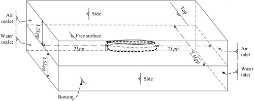
The inlet, top, bottom, and side boundaries are treated as velocity inlets. The hydrostatic pressure is specified at the outlet plane. On the hull and rudder surfaces, the non-slip condition is specified. The pressure resistance fluctuation is usually found to be caused by the wave reflection at the non-physical side boundaries. Therefore, a numerical damping at the side boundaries is applied to remove the fluctuation.

4.4. Mesh generation

The grid structure around the ship is shown in Figure 3. The unstructured predominant hexahedral mesh is applied to discretize the computational domain. Near the ship surface, orthogonal prismatic cells are generated to improve the accuracy of the flow resolution. Since the blended wall function is applied, prism layers are used to achieve y+ values around 30. The free surface, the bow and stern of the hull, and the rudder parts are refined by using volume refinement boxes in grid generation in order to resolve the flow. The virtual disk of the propeller is refined to ensure the proper cell size in the areas where it is needed.

Figure 3. Mesh structure in the regions around the ship. (a) Side view; (b) close up of the stern region; (c) close up of the bow region.

5. Numerical uncertainty analysis

Before proceeding to systematic computation, it is necessary to perform a verification study. In the present study, the verification study is conducted following the Grid Convergence Index (GCI) method developed by Roache (1998) and described in Celik, Ghia, Roache, and Freitas (2008). This method is currently used and recommended by the American Institute of Aeronautics and Astronautics (AIAA). The discretization errors caused by grid size and time step are evaluated for the two dynamic cases, one pure sway and one yaw–drift, as indicated in Table 4, assuming that the numerical uncertainties for the other cases are of the same order.

All mesh quantities are given as percentages in terms of a base size, in order to refine the grid as systematically as possible. The grid refinement is achieved by applying a refinement factor r_G= to the base size. Three grid sets (coarse, medium, fine) are adopted in the study. The fine, the medium, and the coarse grids consist of approximately 2.81M, 1.57M and 0.6M cells, respectively. The refinement ratio of the time step is the same as refined mesh, that is r_t=. Three sets of time steps are T/566, T/400, and T/283, respectively, where T = 1/f is the period of the oscillating motion. The mesh convergence analysis is performed with a fine time step, and the time-step convergence study is executed with a fine grid. The total computing time for coarse, medium, and fine grid density or time step is about 12, 24, and 36 hours, respectively.

The changes in solutions between two successive parameters are defined as: (13) where , , and correspond to the solutions with fine, medium, and coarse input parameters. The subscript k refers to the input parameters (i.e. ‘G’ for grid size and ‘t’ for time step).

The apparent order p_k of the method is expressed by: (14)

The extrapolated values can be calculated by: (15)

The approximate relative error between medium and fine solutions and the extrapolated relative error can be computed as follows: (16) (17)

The fine-grid or fine-time convergence index which represents the numerical uncertainty is calculated by: (18) Traditionally, the verification of the static simulations is focused on constant forces or moments, while the dynamic simulations cover verification of time series for forces and moments on the time level such as in Simonsen and Stern (2008). However, from the ITTC (2014) Guidelines, it can be seen that instead of making the verification on the time series directly, it is recommended to approximate the time series of the forces and moments with FS coefficients, as is done in Sakamoto et al. (2012).

Table 5 summarizes the results of the grid-spacing and time-step convergence study for only Y_c1, Y_s1, Y_c3, N_c1, N_s1, and N_c3 in the pure sway case, since the corresponding hydrodynamic derivatives are obtained from those FS coefficients. As can be seen from Table 5, the lower order FS coefficients (Y_c1, Y_s1, N_c1, and N_s1) have much smaller approximate relative errors, extrapolated relative errors, and uncertainty values than those of higher order FS coefficients (Y_c3 and N_c3) for grid resolution. The numerical uncertainties in the fine-grid solution for those lower order FS coefficients are less than 5%, while for higher order ones they are more than 25%. For the time-step convergence, all of those six coefficients are fairly insensitive to the size of the time step, since the maximum reaches only 3.25%.

Table 5. Mesh and time-step convergence study for the FS coefficients in the pure sway case.

Mesh convergence	p		(%)	(%)	(%)
Yc1	3.93	3.41E-03	3.53	1.20	1.52
Yc3	3.29	2.06E-04	13.84	6.94	8.12
Ys1	10.32	−2.69E-03	0.04	0.00	0.00
Nc1	6.46	1.04E-03	0.76	0.09	0.11
Nc3	2.04	1.02E-04	22.75	18.08	27.58
Ns1	4.41	7.03E-05	14.30	3.81	4.95
Time-step convergence	p		(%)	(%)	(%)
Yc1	0.94	3.43E-03	0.78	1.99	2.53
Yc3	4.13	2.21E-04	2.43	0.76	0.95
Ys1	4.12	−2.69E-03	0.24	0.08	0.09
Nc1	3.53	1.05E-03	0.81	0.34	0.42
Nc3	2.22	8.59E-05	3.00	2.53	3.25
Ns1	4.26	6.70E-05	3.21	0.96	1.19

Table 6 summarizes the results of the grid-spacing and time-step convergence study for some FS coefficients in the yaw–drift case. Like the pure sway case above, the lower order FS coefficients have much smaller uncertainty values than those of higher order ones for both grid and time resolutions. The maximum numerical uncertainty among X_s1, Y₀, Y_s1, N₀, and N_s1 is less than 11% in the mesh convergence study, while it is less than 2% in the time-step convergence study. From the numerical uncertainty analysis, it can be concluded that the lower order FS coefficients have much less numerical uncertainties. Therefore, MRL methods with the 0th- or the 1st-order FS coefficients are preferred to compute the hydrodynamic derivatives in the present study.

Table 6. Mesh and time-step convergence study for the FS coefficients in the yaw–drift case.

Mesh convergence	p		(%)	(%)	(%)
Xc2	2.71	−2.17E-05	5.13	3.41	4.12
Xs1	3.60	−2.80E-04	0.74	0.30	0.37
Y0	3.81	2.34E-03	3.89	1.44	1.77
Yc1	10.61	−3.57E-04	1.47	0.04	0.05
Yc2	3.83	−4.58E-04	9.77	3.66	4.42
Ys1	3.07	9.22E-04	14.05	6.88	9.24
Ys3	3.18	4.23E-05	20.23	11.22	12.61
N0	1.12	7.09E-04	4.13	9.52	10.86
Nc1	5.33	−3.02E-04	3.72	0.69	0.87
Nc2	4.90	−3.08E-06	72.67	13.99	20.34
Ns1	1.42	−1.40E-03	2.78	4.57	5.46
Ns3	1.93	2.30E-07	65.54	222.30	86.22
Time-step convergence	p		(%)	(%)	(%)
Xc2	0.45	−1.83E-05	3.11	22.38	22.86
Xs1	3.39	−2.81E-04	0.30	0.14	0.17
Y0	20.00	2.37E-03	3.47	0.00	0.00
Yc1	0.55	−4.27E-04	4.14	16.44	24.60
Yc2	3.57	−4.57E-04	9.18	3.89	4.69
Ys1	6.25	8.70E-04	10.79	1.38	1.75
Ys3	2.58	3.93E-05	23.70	19.61	20.50
N0	5.08	7.72E-04	3.21	0.67	0.84
Nc1	6.71	−3.01E-04	3.66	0.40	0.50
Nc2	8.64	−2.66E-06	8.66	0.45	0.57
Ns1	4.90	−1.46E-03	2.34	0.53	0.66
Ns3	4.23	−3.57E-07	494.41	307.60	185.21

From the grid and time dependency studies, it can be seen that the approximate relative errors between medium and fine solutions in MRL methods are small, while the computational time is about doubled. Thus a medium grid density is chosen for the subsequent simulations to maintain an affordable computation cost, which contains about 1.6M cells. Besides, the medium time step (T/400) is chosen during the numerical simulation of dynamic captive model tests.

6. Results and discussion

After the verification study, systematic simulations of the captive model tests as listed in Tables 3 and 4 are carried out, and the total computational time required is about 20 days.

6.1. Hydrodynamic forces and moments

The hydrodynamic forces and moments on the ship are the main concern for evaluating the hydrodynamic derivatives. The computation results are validated by comparing with the Experimental Fluid Dynamics (EFD) data from the FORCE Technology’s standard PMM tests (Simonsen, 2014).

6.1.1. Static mode

Figures 4–6 show the computation results of hydrodynamic forces and moments of the static tests in comparison with the EFD data. In general, the overall trend shows that the computation results of the non-dimensional hydrodynamic forces are in good agreement with the experimental data. From Figure 4(a), it can be seen that although the computed trend of longitudinal forces X’ at the lowest speed (Fr = 0.156) for positive drift angle are different from the experimental data, it is almost the same for negative drift angle. The average relative error E (E = [(EFD–CFD)/EFD]100%) for longitudinal forces X’ at Fr = 0.156 is about 8.9%; the standard deviation about the relative error is about 4.9%, which is acceptable. In the static rudder case at larger positive rudder angle and lowest captive speed, some discrepancies between CFD and EFD can be seen for Y’ and N’ (Figure 5(b) and (c)). The discrepancies might be due to the body force model of propeller. The propeller inflow is strongly dependent on the wake field. The wake flow changes significantly at lower speeds and large drift angles due to complex vorticity, while the simplified propeller model does not really reflect the difference in propeller load distribution over the disk. Thus, the predicted distribution of the propeller slipstream velocity that hits the rudder might not be accurate, which will affect the rudder performance and further influence X’, Y’, and N’. The experimental uncertainty could also be one of the causes.

Figure 4. Comparison of the results for the static drift case at different drift angles and captive speeds: (a) X’; (b) Y’; (c) N’.

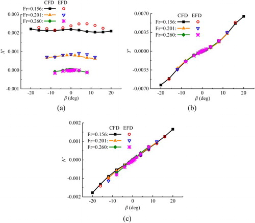
Figure 5. Comparison of the results for the static rudder case at different rudder angles and captive speeds: (a) X’; (b) Y’; (c) N’.

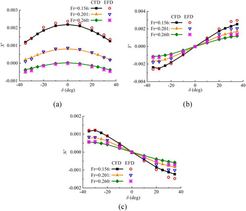
Figure 6. Comparison of the results for the rudder–drift case at different rudder angles, drift angles, and captive speeds: (a) X’; (b) Y’; (c) N’.

For the static drift case, X’ increases when the captive speed decreases. This is because the propeller RPMs are kept constant at service speed self-propulsion point, and the propeller delivers too much thrust at the lower speeds. The three curves of Y’ are almost coincident with each other, the same as those of N’ (see Figure 4(b) and (c)), indicating that the non-dimensional transverse force and yaw moment are not sensitive to captive speed in static drift case. The influence of drift angle on global loads is well captured even at larger drift angles outside the linear region. For the static rudder case, approximately, the computed Y’ and N’ increase linearly with the increase of rudder angle. Y’ and N’ become nonlinear at the rudder angle larger than ± 20° (Figure 5(b) and (c)). For the rudder–drift case, the computed X’, Y’, and N’ at the lower captive speeds (Fr = 0.156, 0.201) are validated by comparing with the experimental data. It can be seen that the slopes of the Y’ and N’ curves are both increasing as the captive speed decreases.

6.1.2. Dynamic mode

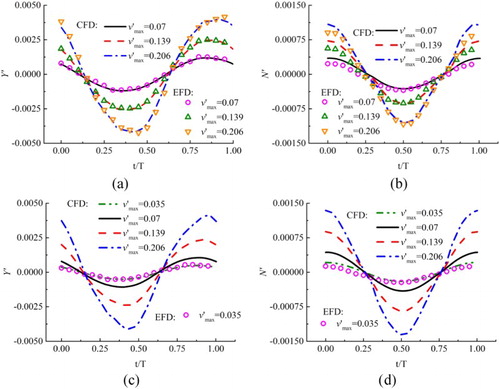
Figure 7 shows the pure sway results at different maximum sway velocity and captive speeds. It can be seen that at the same captive speed, although the trend of the forces is almost the same for different transverse velocities, the amplitude of hydrodynamic forces increases as the sway velocity increases. Overall agreement between CFD and EFD is satisfactory, except the peak values in yaw moments.

Figure 7. Pure sway results at different maximum sway velocities and captive speeds: (a) Y’, Fr = 0.201; (b) N’, Fr = 0.201; (c) Y’, Fr = 0.26; (d) N’, Fr = 0.26.

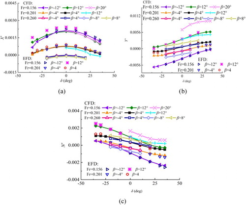
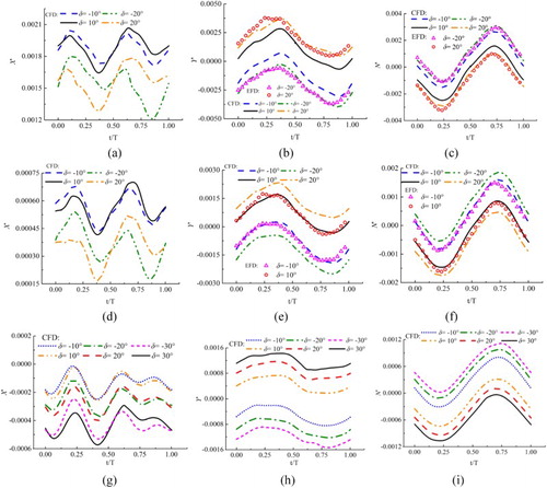
The time histories of forces and moment of pure yaw cases at different captive speeds and yaw rates are depicted in Figure 8. The overall trend shows that the computation results agree well with the experimental data. The amplitude of Y’ and N’ increases as the yaw rate increases at each captive speed. Figure 9 shows the results of the yaw–drift case. Due to the drift angle, asymmetric transverse force and yaw moment can be observed. The changing trend of the hydrodynamic forces is almost the same for different drift angles, but the amplitude of the forces increases as drift angle increases. Some discrepancy can be seen for the longitudinal force coefficients X’ compared with EFD (Figure 9(a) and (d)), which might be due to the body force model for the propeller. The noise in the experiment and the relative small values may also lead to error. Figure 10 shows the results of the yaw–rudder case. Like the yaw–drift case, asymmetric transverse force and yaw moment can be observed.

Figure 8. Pure yaw results at different maximum yaw rates and captive speeds: (a) X’, Fr = 0.156; (b) Y’, Fr = 0.156; (c) N’, Fr = 0.156; (d) X’, Fr = 0.201; (e) Y’, Fr = 0.201; (f) N’, Fr = 0.201; (g) X’, Fr = 0.26; (h) Y’, Fr = 0.26; (i) N’, Fr = 0.26.

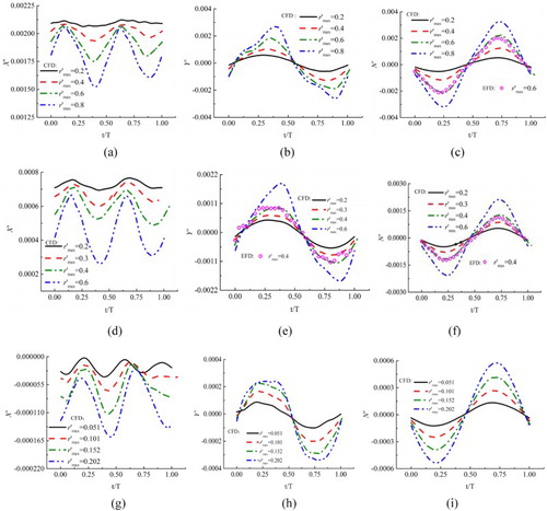
Figure 9. Yaw–drift results at different drift angles and captive speeds: (a) X’, Fr = 0.156; (b) Y’, Fr = 0.156; (c) N’, Fr = 0.156; (d) X’, Fr = 0.201; (e) Y’, Fr = 0.201; (f) N’, Fr = 0.201; (g) X’, Fr = 0.26, and β > 0; (h) Y’, Fr = 0.26, and β > 0; (i) N’, Fr = 0.26, and β > 0; (j) X’, Fr = 0.26, and β  < 0; (k) Y’, Fr = 0.26, and β  < 0; (l) N’, Fr = 0.26, and β  < 0.

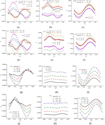
Figure 10. Yaw–rudder results at different rudder angles and captive speeds: (a) X’, Fr = 0.156; (b) Y’, Fr = 0.156; (c) N’, Fr = 0.156; (d) X’, Fr = 0.201; (e) Y’, Fr = 0.201; (f) N’, Fr = 0.201; (g) X’, Fr = 0.26; (h) Y’, Fr = 0.26; (i) N’, Fr = 0.26.

6.2. Simulation of the standard maneuvers

The hydrodynamic derivatives with respect to the rudder angle, sway velocity, and yaw rate are obtained based on the virtual captive model tests. The results are listed in Table 7. It should be noted that for the surge inertia term an empirical value (Simonsen et al., 2012) is chosen, which is about 5% of the non-dimensional mass of the ship. The non-dimensional longitudinal gravity center , ship mass m’, and moment of inertia are calculated (see Table 2) and also given in Table 7.

Table 7. Non-dimensional hydrodynamic derivatives and main particulars (×10⁵).

Coefficients	Values	Coefficients	Values	Coefficients	Values
X'u	−209.70	Y'*	−1.48	N'*	0.70
X'uu	245.76	Y'*u	10.58	N'*u	−4.51
X'uuu	108.67	Y'*uu	7.35	N'*uu	−0.78
X'*	2.83	Y'*uuu	−9.05	N'*uuu	6.97
X'vv	−614	Y'v	−935	N'v	−513
X'vvu	−910.08	Y'vvv	−20916	N'vvv	124
X'rr	−360.00	Y'vu	−4590.39	N'vu	−292.99
X'rru	−386.87	Y'vuu	−1.56	N'vuu	−196.00
X'vr	619.60	Y'r	193.14	N'r	−233.03
X'vru	110.26	Y'ru	−152.11	N'ru	−27.38
X'δδ	−106	Y'ruu	−80.44	N'ruu	−61.61
X'δδu	235.49	Y'rrr	−1229	N'rrr	−1040
X'vδ	66.51	Y'vvr	−1020	N'vvr	−3024
X'vδu	−34.30	Y'vrr	−25,446	N'vrr	−3699
X'rδ	−46.86	Y'δ	257	N'δ	−125
X'rδu	66.64	Y'uδ	−415.49	N'uδ	201.67
	−42.77	Y'uuδ	67.18	N'uuδ	−33.15
m'	855	Y'δδδ	−176	N'δδδ	85.3951
	53.46	Y'vδδ	−532	N'vδδ	248
	−340,500	Y'vvδ	1975	N'vvδ	−938
		Y'rδδ	41.28	N'rδδ	−6.77
		Y'rrδ	1377.64	N'rrδ	−6.65
			−863		22.95
			−18.45		−51.88

Figures 11 and 12 show the simulation results (CFD-Present) of 35° turning circle and 10°/10° and 20°/20° zigzag maneuvers by using the hydrodynamic derivatives listed in Table 7. FRMT from MARIN (FRMT-MARIN) (SIMMAN, 2014), PMM tests, and virtual captive model tests from FORCE Technology (PMM-FORCE and CFD-FORCE) (Otzen & Simonsen, 2014; Simonsen et al., 2012) are also presented for comparison. In PMM-FORCE, the full set of PMM tests (3-DOF) was conducted to evaluate the maneuvers using the standard approach, while in CFD-FORCE, based on the PMM-FORCE data, a reduced test matrix was applied for the PMM computations with the same RANS code as the present study. Both PMM-FORCE and CFD-FORCE were conducted to determine the hydrodynamic derivatives in an integrated mathematical model, which is different from the mathematical model adopted in the present study. According to the SIMMAN Instructions (2014), all the prediction results of standard maneuvers are displayed in full scale values. No scale effect corrections are made on all the forces, i.e. only Froude scaling is applied. This enables direction comparison of results based on different model sizes from different institutions.

Figure 11. Trajectories of ± 35° turning circle maneuvers.

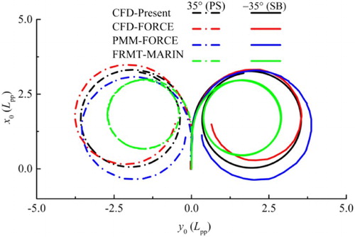
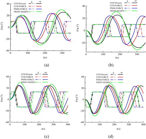
Figure 12. Time histories of heading angle and rudder angle of zigzag maneuvers: (a) 10°/10° zigzag maneuver; (b) −10°/10° zigzag maneuver; (c) 20°/20° zigzag maneuver; (d) −20°/20° zigzag maneuver.

In Table 8, the maneuvering parameters advance (A_D), tactical diameter (D_T), and overshoot angles (OSA) predicted by the system-based methods (CFD-Present, CFD-FORCE, and PMM-FORCE) are compared with those from FRMT (FRMT-MARIN). Table 8 also gives the relative comparison error E (%) of maneuvering parameters from the three system-based methods compared with those from FRMT, defined as (1 − Pred./FRMT)×100%, where ‘Pred.’ denotes the parameter predicted by the system-based methods.

Table 8. Summary of maneuvering parameters including comparison errors with FRMT.

Maneuvers	Parameters	CFD-Present	CFD- FORCE	PMM- FORCE	FRMT- MARIN
	AD (Lpp)	3.29	3.43	2.99	2.93
+35° PS	E (%)	−12.54	−17.18	−2.15	–
	DT (Lpp)	3.56	3.71	3.47	2.63
	E (%)	−35.02	−40.85	−31.73	–
	AD (Lpp)	3.25	3.27	3.24	2.90
−35° SB	E (%)	−12.12	−12.93	−11.90	–
	DT (Lpp)	3.52	3.49	3.82	2.82
	E (%)	−24.64	−23.57	−35.25	–
10°/10°	1st OSA (°)	10.51	7.60	9.30	10.76
	E (%)	2.32	29.37	13.58	–
	2nd OSA (°)	17.15	14.40	12.40	20.23
	E (%)	15.24	28.81	38.70	–
−10°/10°	1st OSA (°)	11.78	9.30	8.00	13.00
	E (%)	9.41	28.46	38.46	–
	2nd OSA (°)	15.40	12.90	13.90	20.85
	E (%)	26.15	38.12	33.33	–
20°/20°	1st OSA (°)	16.69	16.20	17.40	24.40
	E (%)	31.58	33.60	28.68	–
	2nd OSA (°)	17.22	18.00	16.40	20.04
	E (%)	14.11	10.20	18.18	–
−20°/20°	1st OSA (°)	17.34	17.50	17.10	23.22
	E (%)	25.31	24.63	26.35	–
	2nd OSA (°)	16.58	17.30	15.60	21.58
	E (%)	23.18	19.85	27.72	–

From Figure 11 it can be seen that all the system-based prediction methods over-predict obviously the advance and tactical diameter compared with FRMT. The large difference in turning circle maneuver between FRMT and those obtained from virtual or physical captive model tests may be ascribed to many reasons, such as the differences in the selected mathematical models, effect of ‘solidity of captive model tests’, the roll motion, the differences of the propeller models, and model scale effects, etc. (Quadvlieg, 2017). As can be seen in Table 8, all the relative comparison errors of both advance and tactical diameters by the CFD-Present method are smaller than those by CFD-FORCE, but larger than those by PMM-FORCE, except for the tactical diameter in the −35° turning circle maneuver. The maximum and minimum comparison errors of the tactical diameter compared with FRMT occur in the simulations of CFD-FORCE within about −41% for the PS and −24% for the SB, respectively. The comparison error of the tactical diameter in the simulations of CFD-Present for the SB is about −25%, just slightly larger than that of CFD-FORCE. As for the advance, based on an overall quantitative comparison for the two CFD methods, better agreement can be achieved by the CFD-Present method within about −13% minimum relative error for the PS and −12% for the SB. Moreover, all the relative comparison errors of advance (maximum value of E equal to −17%) are smaller than that of tactical diameter (maximum value of E equal to −41%), indicating that the advance is better predicted.

In Table 8, the comparison errors of OSAs by the three system-based methods are positive, demonstrating that all the system-based methods under-predict the 1st and 2nd OSAs compared with FRMT. From Figure 12(a) (10°/10°) and Figure 12(b) (−10°/10°), it can be seen that compared with CFD-FORCE and PMM-FORCE, the 1st and 2nd OSAs predicted by the CFD-Present method show the best agreement with the minimum relative comparison errors of 2.3% and 15.2% for 10°/10°, 9.41% and 26.15% for −10°/10° zigzag maneuvers, respectively. The 1st and 2nd overshoot times predicted by the CFD-Present method are much closer to FRMT. From Figure 12(c) (20°/20°) and Figure 12(d) (−20°/20°), it can be seen that the comparison errors of the three system-based methods show little difference for both 1st and 2nd OSAs. Although the CFD-Present method gives a worse prediction of 1st and 2nd OSAs than PMM-FORCE, it predicts better than FORCE-CFD.

The cause of the differences in maneuvering motion predictions between CFD-FORCE and CFD-Present might be the test matrix reduction in CFD-FORCE and the distinction of the adopted mathematical models between the FORCE methods and present method. Besides, different numerical errors by different CFD methods could decrease the accuracy of maneuvering motion predictions to different extents.

7. Conclusions

By using an unsteady RANS solver, virtual captive model tests including static rudder, static drift, rudder–drift, pure sway, pure yaw, yaw–rudder, and yaw–drift tests at different captive speeds are carried out for the KCS ship model. Firstly, numerical uncertainty analysis is conducted. It is concluded that the values of numerical uncertainty are relatively small for the lower order Fourier coefficients, hence the lower order Fourier coefficients are preferred during the computation of the hydrodynamic derivatives. The computation results of non-dimensional longitudinal force, transverse force, and yaw moment are validated by comparing with the available experimental data. It is demonstrated that the hydrodynamic forces and moments acting on a ship model in the captive model tests can be accurately predicted by using the proposed numerical model except for the longitudinal force in some cases mainly due to the simplified body force model for the propeller.

A full set of 65 linear and nonlinear hydrodynamic derivatives in the 3rd-order Abkowitz model are determined from the virtual captive model test. By using the hydrodynamic derivatives, 35° turning circle and 10°/10°, 20°/20° zigzag maneuvers are simulated, and the maneuvering characteristics of the ship are predicted. For validation of the prediction procedure developed in the present study, the numerical results are compared with the data of free running model tests from MARIN and those of CFD computations and PMM tests from FORCE Technology. From the comparisons it is confirmed that although the present method is less accurate than the PMM-based method overall, it gives a better prediction than the CFD method of FORCE Technology. These results show that the present method is effective in determining the hydrodynamic derivatives in the mathematical model of ship maneuvering motion, and can be used as an alternative to the captive model tests for predicting ship maneuverability at the ship design stage.

However, it should be pointed out that the body force model seems to underestimate the changes of the propeller thrust and torque due to oblique propeller inflow in large drift angle and low speed simulations. Further analysis about the body force model and full propeller model in oblique flow is needed to get more accurate results. Moreover, the present work focuses on 3-DOF maneuvering motions and neglects the roll effect; while in fact ship roll is non-negligible during ship maneuvering, especially for a container ship. Therefore, a 4-DOF model with roll effect should be adopted in a future study. In addition, the present research is carried out at model scale and needs to be extended to full scale. In a future study, the virtual captive model tests can be conducted for models with different scales to investigate possible scale effects on the maneuvering derivatives. In this way, full-scale prediction can be achieved by extrapolation.

Acknowledgements

The authors thank the FORCE Technology in Denmark for providing the benchmark test data.

Disclosure statement

No potential conflict of interest was reported by the authors.

Additional information

Funding

This work was supported by National Natural Science Foundation of China [Grant Numbers 51309152 and 51779140].

References

- Abkowitz, M. A. (1964). Lectures on ship hydrodynamics-steering and manoeuvrability. Lyngby: Hydro- and Aerodynamics Lab.
- Alexandersson, M., Korkmaz, K. B., & Mazza, G. (2017, October). Virtual captive tests with a destroyer hull form. Proceedings of the Numerical Towing Tank Symposium, Wageningen, The Netherlands.
- CD-Adapco. (2014). STAR-CCM+ User Guide.
- Celik, I. B., Ghia, U., Roache, P. J., & Freitas, C. J. (2008). Procedure for estimation and reporting of uncertainty due to discretization in CFD applications. Journal of Fluids Engineering-Transactions of the ASME, 130(7), Article No. 078001.
- Dubbioso, G., Durante, D., Di Mascio, A., & Broglia, R. (2016). Turning ability analysis of a fully appended twin screw vessel by CFD. Part II: Single vs. Twin rudder configuration. Ocean Engineering, 117, 259–271. doi: 10.1016/j.oceaneng.2016.03.001
- Guo, H. P., & Zou, Z. J. (2017). System-based investigation on 4-DOF ship maneuvering with hydrodynamic derivatives determined by RANS simulation of captive model tests. Applied Ocean Research, 68, 11–25. doi: 10.1016/j.apor.2017.08.006
- He, S., Kellett, P., Yuan, Z. M., Incecik, A., Turan, O., & Boulougouris, E. (2016). Manoeuvring prediction based on CFD generated derivatives. Journal of Hydrodynamics, Series B, 28(2), 284–292. DOI: 10.1016/S1001-6058(16)60630-3
- Hirt, C. W., & Nichols, B. D. (1981). Volume of fluid (VOF) method for the dynamics of free boundaries. Journal of Computational Physics, 39(1), 201–225. doi: 10.1016/0021-9991(81)90145-5
- IMO. (2002). Standards for ship manoeuvrability, Resolution MSC. 137(76).
- ITTC. (2011). Guideline on used of RANS tools for manoeuvring prediction (No. 7.5-03-04-01). Retrieved from website: https://ittc.info/media/4204/75-03-04-01.pdf
- ITTC. (2014). Validation and verification of RANS solutions in the prediction of manoeuvring capabilities (No. 7.5-03-04-02). Retrieved from website: https://ittc.info/media/4206/75-03-04-02.pdf
- ITTC, Manoeuvring Committee. (2008, September). Final report and recommendations to the 25th ITTC. Proceedings of 25th International Towing Tank Conference, Fukuoka, Japan.
- Jin, Y., Duffy, J., Chai, S., Chin, C., & Bose, N. (2016). URANS study of scale effects on hydrodynamic manoeuvring coefficients of KVLCC2. Ocean Engineering, 118, 93–106. DOI: 10.1016/j.oceaneng.2016.03.022
- Kijima, K., Katsuno, T., Nakiri, Y., & Furukawa, Y. (1990). On the manoeuvring performance of a ship with the parameter of loading condition. Journal of the Society of Naval Architects of Japan, 168, 141–148. https://doi.org/10.2534/jjasnaoe1968.1990.168_141
- Liu, Y., Zou, L., & Zou, Z. J. (2017). Computational fluid dynamics prediction of hydrodynamic forces on a manoeuvring ship including effects of dynamic sinkage and trim. Proceedings of the Institution of Mechanical Engineers, Part M: J Engineering for the Maritime Environment. Advance online publication. DOI: 10.1177/1475090217734685
- Obreja, D., Nabergoj, R., Crudu, L., & Păcuraru-Popoiu, S. (2010). Identification of hydrodynamic coefficients for manoeuvring simulation model of a fishing vessel. Ocean Engineering, 37(8-9), 678–687. doi: 10.1016/j.oceaneng.2010.01.009
- Ohmori, T. (1998). Finite-volume simulation of flows about a ship in maneuvering motion. Journal of Marine Science and Technology, 3(2), 82–93. DOI: 10.1007/BF02492563
- Otzen, J. F., & Simonsen, C. D. (2014, December). Manoeuvring predictions for the KCS container ship based on experimental and numerical PMM tests. Proceedings of Workshop on Verification and Validation of Ship Manoeuvring Simulation Methods, Copenhagen, Denmark.
- Patankar, S. V., & Spalding, D. B. (1972). A calculation procedure for heat, mass and momentum transfer in three-dimensional parabolic flows. International Journal of Heat and Mass Transfer, 15(10), 1787–1806. doi: 10.1016/0017-9310(72)90054-3
- Quadvlieg, F. H. (2017, January). The importance of benchmarking of manoeuvring prediction methods - Status 2014. Keynote lecture presented at the International Workshop on Ship Manoeuvring and Control, Shanghai, China.
- Quérard, A., Temarel, P., & Turnock, S. (2008, January). Influence of viscous effects on the hydrodynamics of ship-like sections undergoing symmetric and anti-symmetric motions, using RANS. Proceedings of the 27th International Conference on Offshore Mechanics and Arctic Engineering, Estoril, Portugal.
- Roache, P. J. (1998). Verification and validation in computational science and engineering. Albuquerque, NM: Hermosa.
- Sakamoto, N., Carrica, P. M., & Stern, F. (2012). URANS simulations of static and dynamic maneuvering for surface combatant: Part 1. Verification and validation for forces, moment, and hydrodynamic derivatives. Journal of Marine Science and Technology, 17(4), 422–445. doi: 10.1007/s00773-012-0178-x
- Shenoi, R. R., Krishnankutty, P., & Selvam, R. P. (2016). Study of maneuverability of container ship with nonlinear and roll-coupled effects by numerical simulations using RANSE-based solver. Journal of Offshore Mechanics and Arctic Engineering - Transactions of the ASME, 138(4), Article No. 041801.
- Shih, T. H., Liou, W. W., Shabbir, A., Yang, Z., & Zhu, J. (1995). A new k-ϵ eddy viscosity model for high Reynolds number turbulent flows. Computers & Fluids, 24(3), 227–238. DOI: 10.1016/0045-7930(94)00032-T
- SIMMAN. (2008). Workshop on verification and validation of ship manoeuvring simulation methods, Copenhagen, Denmark. Retrieved from http://www.simman2008.dk/
- SIMMAN. (2014). Workshop on verification and validation of ship manoeuvring simulation methods, Copenhagen, Denmark. Retrieved from http://www.simman2014.dk/
- Simonsen, C. D. (2014, December). KCS PMM tests with appended hull, FORCE 2009-SIMMAN 2014. Proceedings of Workshop on Verification and Validation of Ship Manoeuvring Simulation Methods, Copenhagen, Denmark.
- Simonsen, C., Otzen, J., Klimt, C., Larsen, N., & Stern, F. (2012, August). Maneuvering predictions in the early design phase using CFD generated PMM data. Proceedings of 29th Symposium Naval Hydrodynamics, Gothenburg, Sweden.
- Simonsen, C. D., & Stern, F. (2008, April). RANS simulation of the flow around the KCS container ship in pure yaw. Proceedings of Workshop on Verification and Validation of Ship Manoeuvring Simulation Methods, Copenhagen, Denmark.
- Stern, F., Kim, H., Patel, V. C., & Chen, H. (1988). Computation of viscous flow around propeller-shaft configurations. Journal of Ship Research, 32(4), 263–284.
- Stern, F., Yang, J., Wang, Z., Sadat-Hosseini, H., & Mousaviraad, M. (2013). Computational ship hydrodynamics: Nowadays and way forward. International Shipbuilding Progress, 60(1–4), 3–105.
- Strøm-Tejsen, J., & Chislett, M. S. (1966). A model testing technique and method of analysis for the prediction of steering and manoeuvring qualities of surface vessels. Lyngby: Hydro- and Aerodynamics Lab.
- Sun, Y., Su, Y., Wang, X., & Hu, H. (2016). Experimental and numerical analyses of the hydrodynamic performance of propeller boss cap fins in a propeller-rudder system. Engineering Applications of Computational Fluid Mechanics, 10(1), 145–159. DOI: 10.1080/19942060.2015.1121838
- Sung, Y. J., Park, S. H., & Jun, J. H. (2015, September). Prediction of ship manoeuvring behaviors based on virtual captive model tests. Proceedings of 7th International Conference on Marine Simulation and Manoeuvrability, Newcastle, England.
- Sutulo, S., & Guedes Soares, C. (2014). An algorithm for offline identification of ship manoeuvring mathematical models from free-running tests. Ocean Engineering, 79, 10–25. DOI: 10.1016/j.oceaneng.2014.01.007
- Tran Khanh, T., Ouahsine, A., Naceur, H., & El Wassifi, K. (2013). Assessment of ship manoeuvrability by using a coupling between a nonlinear transient manoeuvring model and mathematical programming techniques. Journal of Hydrodynamics, Series B, 25(5), 788–804. doi: 10.1016/S1001-6058(13)60426-6
- Veedu, R. T., & Krishnankutty, P. (2016, June). Numerical investigation on the influence of Froude number on the hydrodynamic derivatives of a container ship. Proceedings of 35th International Conference on Ocean, Offshore and Arctic Engineering, Busan, South Korea.
- Wang, J. H., Zou, L., & Wan, D. C. (2017). CFD simulations of free running ship under course keeping control. Ocean Engineering, 141, 450–464. doi: 10.1016/j.oceaneng.2017.06.052
- Yao, J. X. (2015). On the propeller effect when predicting hydrodynamic forces for manoeuvring using RANS simulations of captive model tests (Doctoral dissertation). Retrieved from DOI: 10.14279/depositonce-4682
- Yasukawa, H., & Yoshimura, Y. (2015). Introduction of MMG standard method for ship maneuvering predictions. Journal of Marine Science and Technology, 20(1), 37–52. DOI: 10.1007/s00773-014-0293-y
- Yoon, H., Simonsen, C. D., Benedetti, L., Longo, J., Toda, Y., & Stern, F. (2015). Benchmark CFD validation data for surface combatant 5415 in PMM maneuvers – part I: Force/moment/motion measurements. Ocean Engineering, 109, 705–734. DOI: 10.1016/j.oceaneng.2015.04.087
- Zhang, S., Zhang, B., Tezdogan, T., Xu, L., & Lai, Y. (2018). Computational fluid dynamics-based hull form optimization using approximation method. Engineering Applications of Computational Fluid Mechanics, 12(1), 74–88. DOI: 10.1080/19942060.2017.1343751
- Zhang, X. G., & Zou, Z. J. (2011). Identification of Abkowitz model for ship manoeuvring motion using ϵ-support vector regression. Journal of Hydrodynamics, Series B, 23(3), 353–360. doi: 10.1016/S1001-6058(10)60123-0
- Zipfel, J. S., Wagner, S., & Abdel-Maksoud, M. (2014, December). RANS simulations of hydrodynamic forces acting on the KVLCC2 tanker. Proceedings of Workshop on Verification and Validation of Ship Manoeuvring Simulation Methods, Copenhagen, Denmark.