Coupling a firefly algorithm with support vector regression to predict evaporation in northern Iran

ABSTRACT

Evaporation accounts for varying shares of water balance under different climatic conditions, and its correct prediction poses a significant challenge before water resources management in watersheds. Given the complex and nonlinear behavior of the evaporation component, and according to the fact that this parameter is not measured at many meteorological stations, at least during some timeframes, and that the meteorological stations measuring this component are not properly distributed in many developing countries, including Iran, the main objective of this work was to predict the evaporation component at two meteorological stations (Rasht and Lahijan) located in Gilan province in northern Iran over the 2006–2016 time period. To that end, those meteorological parameters recorded at the two stations which had the highest impact on evaporation prediction were identified using Pearson correlation coefficient. Selected parameters were then used, under separate scenarios, as inputs to support vector regression (SVR) and SVR model coupled with firefly algorithm (SVR-FA) in order to simulate evaporation values on a daily scale. Evaporation amounts showed the highest correlation with net solar radiation and saturation vapor pressure deficit at Lahijan and Rasht stations, respectively. Root mean square error values of evaporation prediction at testing phase of SVR and SVR-FA ranged from 1.05 to 1.43 and 1.02 to 1.31 mm, respectively, at Lahijan station and from 1.02 to 1.28 and 0.88 to 1.17 mm, respectively, at Rasht station for various scenarios. For underpredicted evaporation data set, the magnitude of RMSE reduction from SVR1 to SVR7 was 27% at Lahijan and 18% at Rasht station; whereas RMSE decrement from SVR-FA1 to SVR-FA7 was 18 and 26 percent at Lahijan and Rasht stations, respectively. This means that for the underpredicted data set, the role of increasing the number of SVR and SVR-FA input parameters in decreasing evaporation prediction error has been more conspicuous at Lahijan and Rasht stations, respectively. Analysis of SVR and SVR-FA performance at various 2-mm intervals of measured evaporation showed that prediction error has generally been increasing with increment of evaporation values, with the highest errors observed at the 8-10 mm interval for both Lahijan and Rasht stations (error rates of 3.42 and 2.42 mm/day at Lahijan and 6.13 and 5.84 mm/day at Rasht station, with SVR1 and SVR-FA1 models, respectively).

KEYWORDS:

• meteorological parameters
• Pearson correlation
• prediction error
• Taylor diagram
• water balance

1. Introduction

The accurate prediction of evaporation is a major challenge in the water resources management of watersheds, and its modeling is of great importance in regions where there is insufficient measured data in terms of either spatial or temporal distribution (Dalkiliç, Okkan, & Baykan, 2014). Evaporation varies depending on the climatic conditions and the availability of surface water bodies in any given area, and its contribution to the discharge of surface water and to atmospheric feed also varies accordingly. This variation affects the design, planning, and management of irrigation systems and water resources (Sudheer, Gosain, Mohana Rangan, & Saheb, 2002; Tabari, Marofi, & Sabziparvar, 2010). The importance of evaporation and its impact on surface water balance is highlighted through its relation to climate change and global warming. The latest outputs of meteorological models suggest that global warming has caused an increase in evaporation from the land surface and surface water bodies, which is anticipated to have a serious impact over time on water resources management and the global population (Mall, Gupta, Singh, Singh, & Rathore, 2006).

In order to predict evaporation, common parameters recorded at meteorological stations are used as the input data for models and simulations. Some of the most important of these parameters include precipitation, wind speed, sunshine hours, and relative humidity (Gavin & Agnew, 2004; Singh & Xu, 1997; Vallet-Coulomb, Legesse, Gasse, Travi, & Chernet, 2001). Dalkiliç et al. (2014) use average temperature, relative humidity, wind speed, minimum air temperature, maximum air temperature, and solar radiation as input parameters for predicting daily evaporation. Their results show that the air temperature and wind speed make the most significant contribution to evaporation prediction, while the least significant contribution is that of relative humidity. Using meteorological data from eight meteorological stations in China for the period 1961 to 2000, Wang, Kişi, Zounemat-Kermani, and Li (2017) present a model which uses air temperature, solar radiation, sunshine hours, relative humidity, and wind speed as its input parameters, and which makes the best prediction of evaporation with a root mean square error (RMSE) of 0.77 mm/day. Kim, Shiri, Kişi, and Singh (2013) use air temperature, wind speed, sunshine hours, relative humidity, and solar radiation as inputs parameters into artificial neural networks (ANNs) for predicting evaporation in South Korea for the period 1985 to 1990, and conclude that air temperature and solar radiation have the most significant impact on daily evaporation prediction. Goyal, Bharti, Quilty, Adamowski, and Pandey (2014) use the main meteorological parameters in the form of four scenarios to predict daily evaporation amounts in India using a support vector regression (SVR) model, and report RMSE values in the range of 1.92 to 2.12 mm/day. It is impossible to model hydrological systems in their entirety due to the complexity of determining all the relevant parameters and the lack of statistical information; thus, the use of simulation methods such as artificial intelligence models is essential (Kişi, Genc, Dinc, & Zounemat-Kermani, 2016; Mosavi, Bathla, & Varkonyi-Koczy, 2017; Wu, Chau, & Li, 2009). The ANN technique is one such method, and its suitability for hydrological research applications is verified by the results of a number of studies (Cigizoglu & Kişi, 2006; Cobaner, Unal, & Kişi, 2009; Guven & Kişi, 2011; Kumar, Raghuwanshi, Singh, Wallender, & Pruitt, 2002; Moghaddamnia, Ghafari Gousheh, Piri, Amin, & Han, 2009; Taormina, Chau, & Sivakumar, 2015; Wu & Chau, 2006). The ANN is an effective tool for modeling nonlinear systems as it does not require complex mathematical equations to be defined for the phenomenon under study. This technique has been widely used for predicting daily evaporation (Guven & Kişi, 2011; Kim et al., 2013; Shirsath & Singh, 2010; Tan, Shuy, & Chua, 2007).

Tabari et al. (2010) reported better performance in an ANN compared to nonlinear regression (with RMSE values of 0.42 and 0.92, respectively) for their evaporation predictions at five meteorological stations in Hamadan province, Iran over the period 1996 to 2005. A sensitivity analysis of their results shows that air temperature and wind speed are the most significant factors in the evaporation prediction. Dalkiliç et al. (2014) predicted daily evaporation in Erzincan, Turkey over the period 2004 to 2010, and found that their ANN (RMSE = 2.27 mm/day) performed better than their Penman model (RMSE = 3.06 mm/day).

According to the literature, predicting evaporation using artificial intelligence algorithms has resulted, in some cases, in superior performance to that of ANNs. Kim et al. (2013) predicted evaporation values on a daily scale at the Daegu and Ulsan meteorological stations in South Korea and report satisfactory performance for all three of their methods; using a generalized regression neural networks model (GRNNM), an adaptive neurofuzzy inference system (ANFIS), and a multilayer perceptron (MLP) neural network model, they obtained RMSEs of 1.665, 1.235, and 1.396 mm/day at Daegu, respectively, and RMSEs of 1.136, 1.215, and 1.364 mm/day at Ulsan, respectively. Allawi and El-Shafie (2016) obtained a correlation coefficient of .96 using an ANFIS model to predict daily evaporation in Johor, southeastern Malaysia. Kişi et al. (2016) used three methods to predict daily evaporation in Turkey, and found that their ANN (RMSE = 2 mm/day) performed better than their chi-squared automatic interaction detector (CHAID, RMSE = 2.06 mm/day) and their classification and regression tree (CR-T, RMSE = 2.07 mm/day), although the differences are not significant.

SVR models have been widely used in watershed hydrological studies and water resources management systems in recent years (Baydaroglu & Koçak, 2014; Cheng-Ping et al., 2011). Their advantages include a fast data-processing speed and higher precision than other classical methods (Baydaroglu & Koçak, 2014). Wu et al. (2009) applied the methods of autoregressive (integrated moving) average (ARIMA), k-nearest neighbors (KNN), ANN, and SVR to streamflow prediction in China over the period 1974 to 2003, finding that the SVR method has the highest precision (with RMSE values of 376.6, 561.5, 299.7, and 148.0 m³/s, respectively). Kişi (2015) used air temperature, wind speed, relative humidity, and solar radiation as the input parameters of an SVR model to predict evaporation in Turkey over the period 2002 to 2006, and the results are indicative of appropriate performance (RMSE = 0.597 mm/day). Goyal et al. (2014) compared the daily evaporation values predicted by four methods for Jharkhand state, India, and found that the SVR (RMSE = 1.92 mm/day) and fuzzy logic (RMSE = 1.95 mm/day) methods produced better estimates than the ANN (RMSE = 2.34 mm/day) and ANFIS (RMSE = 2.94 mm/day) methods.

Optimization algorithms can be effective for optimizing the training of artificial intelligence models (Chau, 2007; Chen, Chau, & Busari, 2015; Gholami, Chau, Fadaee, Torkaman, & Ghaffari, 2015). The firefly algorithm is a relatively novel optimization technique which has two advantages over other similar algorithms. First, it is based on attraction, and attractiveness decreases with distance. This means that the entire population is automatically divided into subgroups which swarm around local optima until eventually the best solution can be found. Second, these subgroups enable the firefly algorithm to simultaneously find all optimal modes (Yang & He, 2013). Studying groundwater contamination, Kazemzadeh-Parsi, Daneshmand, Ahmadfard, and Adamowski (2015) compared a finite-element method (FEM) numerical solution and a modified firefly algorithm with conventional optimization methods (such as a genetic algorithm), and presented their optimized model as an effective tool that is applicable to the remediation and management of contaminated aquifers. In their study of water-level fluctuations in Urmia lake in Iran, Kişi et al. (2015) conclude that their firefly algorithm and SVR method produced better results than their ANN and genetic algorithm, and that the SVR method coupled with the firefly algorithm can be used as a new model and tool for defining various strategies to predict the lake's water level. Ghorbani et al. (2017) utilized SVR and SVR coupled with a firefly algorithm for predicting the field capacity (FC) and permanent wilting point (PWP) of 215 soil samples collected from the East Azerbaijan province in Iran, finding that the coupled method performed better than the SVR method. The FC predictions produced RMSE values of 18.36 and 8.74 mm/m for the SVR and coupled methods, respectively, and the PWP predictions produced RMSE values of 21.75 and 10.61 mm/m for the SVR and coupled methods, respectively.

The accurate identification and prediction of the components of the hydrological cycle is essential to designing, operating, and analyzing effective water resources systems. The process of evaporation is a fundamental component of the hydrological cycle, but evaporation is subject to nonlinear change and there is a lack of measured evaporation data in many meteorological stations for certain time periods, a problem that is further compounded by the uneven spatial distribution of the stations. Bearing all of this in mind, the main objective of this study is to use an SVR model and a hybrid SVR-based firefly algorithm (SVR-FA) model to simulate the evaporation over the period 2006 to 2016 for the Rasht and Lahijan meteorological stations in Gilan province, northern Iran.

2. Method

2.1. Data collection sites

In this study, the main meteorological parameters recorded at the Rasht and Lahijan stations during the period 2006 to 2016 were used to estimate daily evaporation values using the SVR and SVR-FA methods. The maximum air temperature, mean relative humidity, precipitation, sunshine hours, wind speed, saturation vapor pressure deficit, and net solar radiation were selected based on the maximum values of the Pearson correlation coefficients to predict the amount of evaporation in seven different scenarios. The daily measured values of these parameters (over the period 2006 to 2016) were used. After analyzing the data, outlier values were eliminated from the data set. The selected data set was standardized using Eq. (1) below prior to being fed into the models. A total of 3155 and 3296 data points from the Lahijan and Rasht stations, respectively, were used in the modeling procedure. The recorded meteorological parameters and their ranges are presented in Table 1.

Table 1. Climatic parameters recorded at the Lahijan (Rasht) stations over the time period covered in this study.

Parameter	Min	Max	Mean	SD	CV
Tmax (°C)	−0.40 (−1.40)	37.80 (38.00)	21.14 (21.04)	8.25 (8.42)	0.39 (0.40)
RH (%)	19.50 (16.00)	100.00 (100.00)	78.71 (80.57)	10.5 (9.80)	0.13 (0.12)
P (mm)	0.00 (0.00)	134.20 (145.70)	3.83 (3.49)	10.52 (10.85)	2.74 (3.10)
SSH (h)	0.00 (0.00)	12.50 (13.40)	5.07 (4.80)	4.19 (4.21)	0.82 (0.87)
Wind speed (m.s^−1)	0.00 (0.00)	25.00 (20.00)	4.57 (4.26)	2.55 (1.80)	0.55 (0.42)
es−ea (kPa)	0.00 (0.00)	2.65 (2.59)	0.50 (0.47)	0.39 (0.37)	0.78 (0.78)
Rn (MJ.m^−2day^−1)	1.23 (1.96)	18.52 (17.44)	7.87 (7.70)	4.70 (4.16)	0.59 (0.54)
E (mm.day^−1)	0.00 (0.10)	10.00 (11.40)	2.70 (2.40)	2.24 (1.91)	0.83 (0.79)

Note: E = evaporation; e_s−e_a = saturation vapor pressure deficit; P = precipitation; RH = relative humidity; R_n = net solar radiation; SSH = sunshine hours; T = temperature; U₂ = wind speed.

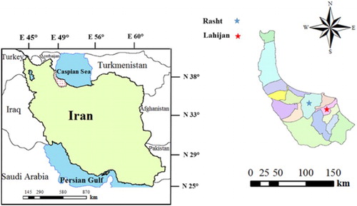
The Lahijan synoptic station is located at a latitude of 37°11'N, a longitude of 50°1'E, and an elevation of 34.2 m above sea level. The Rasht synoptic station is located at a latitude of 37°27'N, a longitude of 49°58'E, and an elevation of 24.9 m above sea level (Figure 1). The average temperature and sunshine hours measured over the time period covered in this study are 16.9°C and 5.22 h at Lahijan and 16.9°C and 6.50 h at Rasht. The average values of annual precipitation recorded are 1399 and 1278 mm/year at Lahijan and Rasht, respectively, and the average daily evaporation rates are 2.7 and 2.4 mm/day at Lahijan and Rasht, respectively. The evaporation amounts range from 0 to 10 mm/day at Lahijan and 0 to 11.4 mm/day at Rasht.

Figure 1. Location of the study area and meteorological stations from which the measurement data were obtained.

2.2. Evaporation prediction

2.2.1. Support vector regression (SVR)

SVR is a set of supervised learning methods that can be used for classification and regression analysis. Introduced by Vapnik and Chervonenkis in 1974 and founded upon statistical learning theory, this method is based on dual classification in the arbitrary feature space and hence is well suited to prediction problems (Jha & Hayashi, 2014; Pai & Hong, 2007; Yoon, Jun, Hyun, Bae, & Lee, 2011).

2.2.2. The firefly algorithm

The firefly algorithm is a bio-inspired algorithm introduced by Yang in 2009 which simulates the social behavior of fireflies. These insects flash light, and each species has its own flash pattern. The attractiveness of a firefly is proportional to its light intensity or brightness. Taking the light intensity of each individual insect as the objective function, the social behavior of fireflies can be modeled as an optimization algorithm (Yang & He, 2013).

2.2.3. Coupling SVR with a firefly algorithm

Not only can SVR implicitly detect complex nonlinear relationships between independent and dependent variables, it also has the ability to detect all possible interactions between predictor variables (Goyal et al., 2014). The firefly algorithm is robust and efficient compared to other metaheuristic algorithms’ local and global searches. It also has good exploitation capabilities and can find better solutions because fireflies come together more closely around the optimal solution, as many candidates (fireflies) gather near to the optimal solution (Ghorbani et al., 2017). Considering the nonlinear trend of variation in evaporation, combining SVR with the firefly algorithm produces a new method which inherits the predictive abilities of SVR and the optimization capabilities of the firefly algorithm. This new method can make predictions with high accuracy at a reasonable speed. The general advantages of combining these two approaches are as follows:

1. It avoids having to explain the complex and nonlinear behaviors of predictive and predicted factors – in the present case, the process of evaporation.

2. It prevents the scope of the optimization algorithm from being trapped in local minima, thanks to the ability to find local as well as global solutions.

3. It simultaneously takes advantage of SVR models’ predictive power and firefly algorithms’ optimization potential in order to obtain the best results.

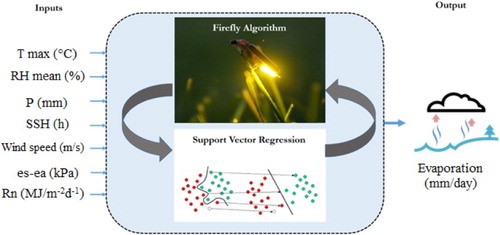
The SVR and SVR-FA models were used in seven different scenarios with various inputs (Table 2 and Figure 2), and the results were compared with the measured evaporation values. A set of daily evaporation values from the period 2006 to 2016 was randomly selected for training and testing the SVR and SVR-FA models, with 2405 and 750 data points used from Lahijan and 2502 and 794 data points from Rasht, respectively. In order to achieve better and faster learning, the meteorological data were normalized between 0 and 1 before being input into the two models and then converted back to their initial values after modeling. The equation used for the normalization process is: (1) where X_i is the measured data, X_n is the standardized data, and X_max and X_min are the maximum and minimum data points, respectively. The computational procedures, including the development of the SVR and SVR-FA models, were implemented in a MATLAB (The MathWorks, 2012) environment, and parameters of the kernel function were optimized through trial and error.

Figure 2. Schematic structure of the SVR and SVR-FA models used for evaporation prediction.

2.3. Performance evaluation

Two statistical indices – the root mean square error (RMSE) and the determination coefficient R² – were used to evaluate the performance of the two modeling approaches: (2) (3) where , , and are the observed, predicted, average observed, and average predicted values of evaporation, respectively.

2.3.1. Taylor diagram

Taylor (2001) introduced a single diagram to summarize multiple aspects of model evaluation indices, including the RMSE and correlation coefficient values, and recommended its use in natural science and hydrology studies for evaluating models’ performance. Taylor diagrams can highlight the accuracy of models’ predictions by comparing the measured and predicted values through visualizing a series of points on a polar plot. The azimuth angle of the diagram shows the correlation coefficient between the measured and predicted values, and the radial distance from the reference point represents the ratio of normalized standard deviation of the simulation from the measured values.

3. Results and discussion

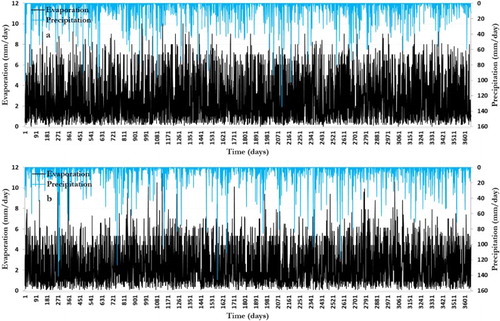
The trend of variation in measured evaporation values, which directly depends on some of the climatic parameters and is indirectly a function of time, along with the average recorded values of this component (Table 1) highlight its role in the water balance in the studied area. Evaporation values as high as about 10 mm/day were recorded at both stations, thus making the importance of generating accurate predictions even more evident. The evaporation that occurs on land largely depends on the soil’s moisture content, especially in the top layers, which are fed by irrigation and/or precipitation. Changes in precipitation are therefore expected to have a significant effect on the evaporation that takes place in the surface soil. The situation is different for surface water bodies, as precipitation does not play a significant role (except when the water level is so low that precipitation will significantly increase it), while other climatic factors – such as the received solar radiation and the humidity – can limit or intensify evaporation. Figure 3 shows the relationship between the precipitation and evaporation measured at the Rasht and Lahijan stations, which are both located in a high-precipitation area of Iran – the average precipitation at Rasht and Lahijan is 1278 and 1399 mm/year, respectively, compared with an average of 250 mm/year for the entire country – so precipitation cannot be considered a significant factor. As shown in Figure 3, not only did an increase in precipitation fail to result in higher amounts of evaporation, but lower precipitation (that is, in the warm season when the received solar radiation is higher) has been accompanied by increased evaporation.

Figure 3. Relation between precipitation and evaporation for the selected time period in this study (days): (a) Lahijan and (b) Rasht.

3.1. Correlation between evaporation and meteorological parameters

Pearson correlation coefficients were used to find the climatic parameters exhibiting the highest impact on the evaporation predictions, and the results are presented in Tables 3 and 4 (all of the correlation coefficients are significant at 95%, p ≤ .05). It can be seen that the evaporation is directly affected by the temperature and inversely affected by the relative humidity at both stations. The maximum temperature and average relative humidity were selected as inputs for the models based on the Pearson correlation coefficient values. As expected due to the climatic conditions of the study area, the evaporation showed a high correlation with the number of sunshine hours, saturation vapor pressure deficit and net solar radiation, with the net solar radiation and saturation vapor pressure deficit exhibiting the highest correlation coefficients for the Lahijan and Rasht stations, respectively. The results presented in Tables 3 and 4 confirm those of Figure 3, showing that precipitation plays an insignificant role in estimating the evaporation component for the data collected at both stations. Previous studies show that the air temperature, relative humidity, wind speed, sunshine hours, and solar radiation are some of the most important predictors of evaporation (Dalkiliç et al., 2014; Goyal et al., 2014; Kim et al., 2013; Piri, Mohammadi, Shamshirband, & Akib, 2016; Wang, Kişi, Zounemat-Kermani, & Gan, 2016).

Table 2. Various scenarios considered as inputs of the models.

Scenario	Input parameters	SVR	SVR-FA
1	Tmax	1	1
2	Tmax, RHmean	2	2
3	Tmax, RHmean, Precipitation	3	3
4	Tmax, RHmean, Precipitation, Sunshine	4	4
5	Tmax, RHmean, Precipitation, Sunshine, Wind speed	5	5
6	Tmax, RHmean, Precipitation, Sunshine, Wind speed, es−ea	6	6
7	Tmax, RHmean, Precipitation, Sunshine, Wind speed, es−ea, Rn	7	7

Note: e_s−e_a = saturation vapor pressure deficit; RH_mean = mean relative humidity; R_n = net solar radiation; T_max = maximum temperature.

Table 3. Pearson correlation coefficient values between the main meteorological parameters measured at the Lahijan station.

	Tmax	Tmin	Tmean	RHmax	RHmin	RHmean	Sunshine	es−ea	Rn	Evaporation
Tmax		0.831	0.963	−0.379	−0.549	−0.568	0.583	0.845	0.862	0.770
Tmin			0.950	−0.269	−0.088	−0.156	0.193	0.596	0.756	0.577
Tmean				−0.342	−0.349	−0.393	0.420	0.762	0.849	0.711
RHmax					0.457	0.683	−0.262	−0.664	−0.295	−0.436
RHmin						0.961	−0.724	−0.761	−0.420	−0.566
RHmean							−0.674	−0.830	−0.436	−0.598
Sunshine								0.647	0.708	0.693
es−ea									0.759	0.807
Rn										0.836

Note: e_s−e_a = saturation vapor pressure deficit; RH_max = maximum relative humidity; RH_mean = mean relative humidity; RH_min = minimum relative humidity; R_n = net solar radiation; T_max = maximum temperature; T_mean = mean temperature; T_min = minimum temperature.

3.2. Evaporation prediction

The evaporation values measured at the Lahijan and Rasht stations, and those predicted by the SVR and SVR-FA models at the testing phase, are shown in Figures 4 and 5. The RMSEs and coefficients of determination between the measured and predicted evaporation amounts for both stations in both the training and testing phases are presented in Table 5, which shows that for both the training and testing phases for both stations, the RMSEs of the evaporation prediction decrease as the number of model inputs increase, although the magnitude of the decrement varies for different meteorological parameters. For the Lahijan station, using the SVR model in the training phase, the highest RMSE decrease occurs for the scenarios in which the saturation vapor pressure deficit, sunshine hours, and net solar radiation are added to the set of input parameters (the RMSE decreases by 9.8, 8.2, and 8.1%, respectively). In the testing phase, the saturation vapor pressure deficit and sunshine hours are the parameters with the most significant roles in estimating evaporation, resulting in decreases of 9.7 and 7.4% in the RMSE, respectively. For the SVR-FA model, the addition of the sunshine hours and relative humidity to the input parameters in the training phase reduces the prediction error by approximately 10.5 and 9.8%, respectively, whereas in the testing phase, only the addition of the relative humidity results in a relatively significant decrease (9.0%) compared to other scenarios.

Figure 4. Measured evaporation amounts versus evaporation values predicted by SVR (black circles) and SVR-FA (blue circles) for different scenarios in Lahijan station and 1:1 line (dash line).

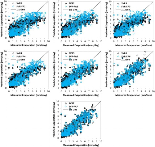
Figure 5. Measured evaporation amounts versus evaporation values predicted by SVR (black circles) and SVR-FA (blue circles) for different scenarios in Rasht station and 1:1 line (dash line).

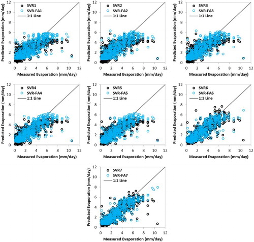
For the Rasht station, for both the SVR and SVR-FA models, the addition of the saturation vapor pressure deficit and the net solar radiation to the input parameters brings about the highest error reduction in the training and testing phases; the addition of these parameters decreases the RMSE by 8.2 and 11.7% in the SVR model, respectively, and by 8.4 and 11.1% in the SVR-FA model, respectively. A comparison of Figures 4 and 5, as well as the results in Table 5, indicates that for the same scenarios, the SVR-FA model provides more accurate predictions than the SVR models for both stations in both the training and testing phases, with the highest RMSE decrement from SVR to SVR-FA occurring in the testing phase in the third scenario for the Lahijan station (approximately 14.0%) and the seventh scenario for the Rasht station (approximately 13.7%). In a study conducted to predict daily evaporation over the period 1987 to 1990 in California, Kişi (2006) showed that the temperature and solar radiation had the highest impact on the estimation of this component, whereas the wind speed and precipitation had the lowest impact.

Table 4. Pearson correlation coefficient values between the main meteorological parameters measured at the Rasht station.

	Tmax	Tmin	Tmean	RHmax	RHmin	RHmean	Sunshine	es−ea	Rn	Evaporation
Tmax		0.875	0.972	−0.232	−0.545	−0.533	0.599	0.834	0.478	0.744
Tmin			0.964	−0.211	−0.188	−0.220	0.300	0.646	0.339	0.636
Tmean				−0.229	−0.390	−0.398	0.474	0.770	0.427	0.716
RHmax					0.394	0.610	−0.153	−0.531	−0.174	−0.322
RHmin						0.968	−0.675	−0.788	−0.484	−0.537
RHmean							−0.622	−0.823	−0.465	−0.550
Sunshine								0.650	0.691	0.632
es−ea									0.539	0.779
Rn										0.633

Note: e_s−e_a = saturation vapor pressure deficit; RH_max = maximum relative humidity; RH_mean = mean relative humidity; RH_min = minimum relative humidity; R_n = net solar radiation; T_max = maximum temperature; T_mean = mean temperature; T_min = minimum temperature.

Table 5. SVR and SVR-FA RMSE and correlation coefficient values in the training (testing) phases for the seven scenarios.

	Lahijan		Rasht
	RMSE	R^2	RMSE	R^2
SVR1	1.44 (1.43)	0.60 (0.61)	1.23 (1.28)	0.59 (0.60)
SVR2	1.36 (1.35)	0.65 (0.66)	1.15 (1.24)	0.63 (0.62)
SVR3	1.34 (1.34)	0.66 (0.67)	1.15 (1.24)	0.63 (0.62)
SVR4	1.23 (1.24)	0.72 (0.71)	1.11 (1.19)	0.66 (0.65)
SVR5	1.22 (1.23)	0.72 (0.72)	1.10 (1.18)	0.67 (0.66)
SVR6	1.10 (1.11)	0.76 (0.76)	1.01 (1.08)	0.71 (0.71)
SVR7	1.01 (1.05)	0.80 (0.78)	0.95 (1.02)	0.75 (0.74)
SVR-FA1	1.32 (1.31)	0.66 (0.66)	1.13 (1.17)	0.64 (0.65)
SVR-FA2	1.19 (1.19)	0.72 (0.72)	1.05 (1.11)	0.69 (0.68)
SVR-FA3	1.14 (1.15)	0.74 (0.74)	1.05 (1.11)	0.69 (0.69)
SVR-FA4	1.02 (1.10)	0.79 (0.76)	1.01 (1.07)	0.72 (0.71)
SVR-FA5	0.99 (1.08)	0.80 (0.77)	0.99 (1.06)	0.72 (0.72)
SVR-FA6	1.00 (1.06)	0.80 (0.78)	0.94 (0.99)	0.75 (0.76)
SVR-FA7	0.96 (1.02)	0.82 (0.79)	0.83 (0.88)	0.81 (0.81)

A look at the days when the evaporation amount is underpredicted or overpredicted (Table 6) shows that at both the Lahijan and Rasht stations higher input numbers resulted in lower prediction errors for both the SVR and SVR-FA models. This is the case with the entire set of evaporation data (Table 5), except for the SVR-FA for Lahijan, which shows a diminutive increment in prediction errors from SVR-FA5 to SVR-FA6 in the underpredicted data set and from SVR-FA4 to SVR-FA5 in the overpredicted data set. For the Lahijan station, the lowest and highest differences between the numbers of days with underprediction or overprediction of evaporation amounts are 6 (SVR7) and 70 (SVR3) days for the SVR models and 6 (SVR-FA6) and 38 (SVR-FA7) days for the SVR-FA models, indicating that the difference between the numbers of underpredicted and overpredicted days is lower for the SVR-FA models. For the Rasht station, the values are 4 (SVR1) and 50 (SVR6) days for the SVR models and 8 (SVR-FA5) and 58 (SVR-FA1) days for the SVR-FA models. Another important point drawn from Table 6 is that at both stations and in all scenarios, both the SVR and SVR-FA models performed better on the days when the evaporation was overpredicted. For the Lahijan station, the lowest and highest RMSE decrements between the underpredicted and overpredicted sets are approximately 14.3% (SVR1) and 19.4% (SVR3) for the SVR models and 7.3% (SVR-FA1) and 21.3% (SVR-FA4) for the SVR-FA models. For the Rasht station, these values are approximately 27.9% (SVR-FA2) and 38.5% (SVR-FA7) for the SVR models and 32.7% (SVR-FA7) and 40.0% (SVR-FA4 and SVR-FA6) for the SVR-FA models. A comparison of the above figures indicates that the reduction in prediction errors for both the SVR and SVR-FA models between the underpredicted and overpredicted sets is higher for the Rasht station.

Table 6. SVR and SVR-FA RMSE values and number of underpredicted or overpredicted days (n) in the testing phases for the seven scenarios at the Lahijan (Rasht) stations.

	Underprediction		Overprediction
Model	RMSE	n	RMSE	n
SVR1	1.54 (1.48)	355 (399)	1.32 (1.06)	395 (395)
SVR2	1.49 (1.43)	349 (381)	1.21 (1.03)	401 (413)
SVR3	1.49 (1.43)	340 (374)	1.20 (1.03)	410 (420)
SVR4	1.36 (1.41)	350 (373)	1.12 (0.95)	400 (421)
SVR5	1.35 (1.38)	346 (385)	1.12 (0.95)	404 (409)
SVR6	1.20 (1.27)	381 (422)	1.00 (0.82)	369 (372)
SVR7	1.13 (1.22)	378 (407)	0.95 (0.75)	372 (387)
SVR-FA1	1.36 (1.41)	387 (368)	1.26 (0.92)	363 (426)
SVR-FA2	1.28 (1.33)	360 (372)	1.09 (0.88)	390 (422)
SVR-FA3	1.24 (1.33)	367 (375)	1.07 (0.86)	383 (419)
SVR-FA4	1.22 (1.32)	371 (378)	0.96 (0.79)	379 (416)
SVR-FA5	1.14 (1.28)	382 (401)	1.02 (0.77)	368 (393)
SVR-FA6	1.15 (1.20)	372 (387)	0.98 (0.72)	378 (407)
SVR-FA7	1.12 (1.04)	356 (381)	0.93 (0.70)	394 (413)

Although the distribution of the predicted evaporation values compared to the distribution of the measured values and the 1:1 line (Figures 4 and 5) partially depicts the performance of the SVR and SVR-FA models for both stations, the authors attempted to further examine their performance in more detail. If the average of the measured evaporation amounts in each station is considered as a threshold value of this component, Figure 6 shows the error rates of both the SVR and SVR-FA models when predicting evaporation values that are lower or higher than this threshold. However, the difference in the performance of the two models in predicting evaporation values lower and higher than the threshold (average measured evaporation at each station) is more evident for the Rasht station, which is indicative of the different behaviors of the SVR and SVR-FA models in predicting various evaporation intervals at the Rasht station. Overall, the highest prediction error is observed for the Rasht station, for evaporation amounts higher than the average.

Figure 6. RMSE values of SVR and SVR-FA models with different scenarios related to measured evaporation amounts higher and lower than average in Lahijan (circle) and Rasht (triangle) stations.

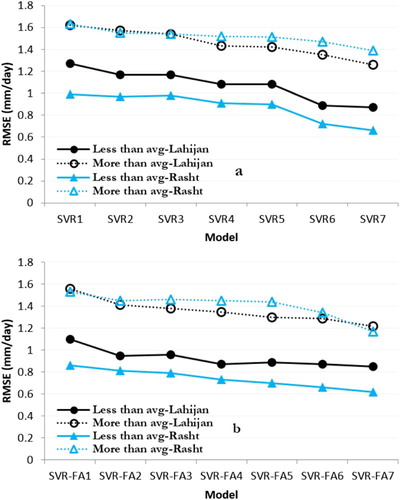
As shown in Figure 6, both models performed better when predicting evaporation amounts lower than the mentioned threshold compared to those above thresholds. For a better analysis of the results, measured values from each station were divided into five 2-mm intervals and the evaporation prediction error rates of both models were calculated for each interval in order to determine the intervals with the highest prediction errors (Figure 7).

Figure 7. RMSE values (mm/day) for predicting evaporation in Lahijan station (two top figures) and Rasht station (two bottom figures) by SVR and SVR-FA models for 2-mm intervals of evaporation.

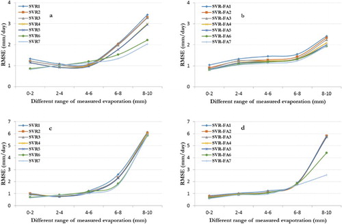
Figure 7 shows that with both models for both stations, the magnitude of the prediction errors generally increases at higher evaporation intervals, with the highest rates of error increment observed in the 6–8 and >8 intervals. With the SVR model and the 0–6 mm interval at Lahijan, however, the prediction errors decreased for higher measured evaporation values, although this decrease is not significant. Another important point understood from Figure 7 is that the influence of having more input parameters on the reduction of the error rates of the models is most evident with the higher evaporation values (especially above 8 mm).

Figure 8 shows the results of the Taylor diagram analysis for the evaporation prediction for the Lahijan and Rasht stations in the training (left) and testing (right) phases. The reference point in a Taylor diagram is determined according to the standard deviation of the data, which here is approximately 2.24 and 1.91 at the Lahijan and Rasht stations, respectively, reflecting the wider range of data at the former station. This is also evident from the wider scattering of the statistical indices of the SVR and SVR-FA models (Figure 8). Each point in this diagram represents the performance of a particular model, and being closer to the reference point means that the model has made a more accurate prediction. Accordingly, for both stations in both the training and testing phases, the SVR and SVR-FA models had the highest and the lowest error rates, respectively, although the range of RMSE changes in the testing phase is higher at the Lahijan station than at the Rasht station.

Figure 8. Statistical indices including standard deviation, correlation coefficient and RMSE in the form of Taylor diagram for SVR and SVR-FA models in Lahijan (training Phase)(a), Lahijan (testing Phase)(b), Rasht (training phase)(c) and Rasht (testing phase)(d).

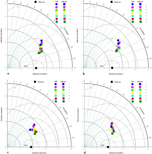
For the Lahijan station in the training phase, the RMSEs range from 0.96 to 1.44 for SVR-FA7 and SVR1, and the coefficient of determination varies from .60 to .82 for SVR1 and SVR-FA7, respectively (Table 5 and Figure 8), whereas in the testing phase the RMSEs and coefficients of determination are in the range of 1.02 to 1.43 and .61 to .79, respectively, for SVR1 and SVR-FA7. The lower error rates for SVR4, SVR5, SVR6 and SVR7 compared to SVR-FA1 (Table 5 and Figure 8) emphasize the importance of the number and type of inputs used in the models in this study, and disprove the hypothesis that a hybrid firefly algorithm always leads to better results than SVR. Increasing the number of inputs reduces the prediction error, especially in case of SVR models. Comparisons between SVR-FA1 and SVR-FA7 and between SVR1 and SVR7 shows 22 and 27% decreases in the RMSEs, respectively. On the other hand, comparing the performance of SVR1 with SVR-FA1 and SVR7 with SVR-FA7 (showing approximately 8 and 3% decreases in the RMSEs, respectively) indicates that the difference between the SVR and SVR-FA models is more evident when using fewer input parameters, and that the difference in performance between the two types of model decreases as the number of inputs increases. In other words, the difference in performance between the SVR and SVR-FA models is more apparent when fewer measured meteorological parameters are available to input into them.

For the Rasht station, the RMSE values are in the range of 0.83 to 1.23 in the training phase and 0.88 to 1.28 in the testing phase for SVR-FA7 and SVR1, respectively, and the coefficient of determination values are in the range of .59 to .81 in the training phase and .60 to .81 in the testing phase for SVR1 and SVR-FA7, respectively. The Taylor diagrams of the models for the Rasht station (Figure 8) show that SVR6 and SVR7 performed better than SVR-FA1. A comparison of the percentages of the RMSE changes in the validation set indicates that the SVR-FA models are more sensitive to an increase in the number of inputs than the SVR models, with the increased number of inputs (changing from the first to seventh scenarios) resulting in 25 and 20% decreases in the RMSEs for the SVR-FA and SVR models, respectively. The behavior of the SVR and SVR-FA models with various inputs for the Rasht station is different from that for the Lahijan station. SVR-FA1 resulted in an 8.5% decrease in the RMSE compared with SVR1, which is comparable to the corresponding value at the Lahijan station (about 8.4%); however, using SVR-FA7 reduced the RMSE by about 13.7% compared to SVR7, which is approximately five times greater than that observed for the Lahijan station. In other words, the advantage of the SVR-FA models over the SVR models, as reflected in the RMSE decrements, is clearer with higher numbers of inputs for the Rasht station (changing SVR7 to SVR-FA7 vs. changing SVR1 to SVR-FA1) but with lower input numbers for the Lahijan station (changing SVR1 to SVR-FA1 vs. changing SVR7 to SVR-FA7).

4. Conclusion

Unfortunately, few studies have been conducted on the application of hybrid algorithms such as the SVR-FA for evaporation prediction, despite the great importance of this component in understanding the water balance in watersheds. In some developing countries, including Iran, many meteorological stations do not record evaporation – thus, using novel hybrid algorithms to predict evaporation can be a useful alternative. The aim of this study was to assess the performance of SVR and SVR-FA models in predicting daily evaporation amounts at the Lahijan and Rasht stations in northern Iran. According to the Pearson correlation coefficient values, the solar radiation and saturation vapor pressure deficit show the highest correlation with the evaporation amounts at Lahijan and Rasht, respectively. Identifying the climatic parameters with the highest impact on evaporation prediction and using them as inputs for the SVR and SVR-FA models in seven different scenarios showed that the prediction error decreases as the number of inputs increases. For the Lahijan station, in the testing phase the prediction errors (mm/day) decreased from 1.43 (SVR1) to 1.05 (SVR7) in the SVR models and from 1.31 (SVR-FA1) to 1.02 (SVR-FA7) in the SVR-FA models. For the Rasht station, in the testing phase the prediction errors (mm/day) decreased from 1.28 (SVR1) to 1.02 (SVR7) in the SVR models and from 1.17 (SVR-FA1) to 0.88 (SVR-FA7) in the SVR-FA models. For the Lahijan station, the coefficient of determination varies from approximately .61 (SVR1) to .78 (SVR7) for the SVR models and from .66 (SVR-FA1) to .79 (SVR-FA7) for the SVR-FA models. For the Rasht station, the coefficient of determination varies from approximately .60 (SVR1) to .74 (SVR7) for the SVR models and from .65 (SVR-FA1) to .81 (SVR-FA7) for the SVR-FA models. Using the average measured evaporation values for each station as a threshold value, both the SVR and SVR-FA models provided more appropriate results when predicting evaporation amounts lower than the threshold. The highest variation in performance for the seven scenarios (reduction of prediction error) for both the SVR and SVR-FA models (excluding the SVR model for the Rasht station) is observed at the 8–10 mm/day interval of measured evaporation amounts. Future research could conduct comparisons between the results from the various empirical methods described in the literature with the results of the algorithms used in the present study, as well as with other hybrid optimization algorithms, in order to scrutinize their performance in the area of watershed water resources management.

Disclosure statement

No potential conflict of interest was reported by the authors.

ORCID

Roozbeh Moazenzadeh http://orcid.org/0000-0002-1057-3801

Babak Mohammadi http://orcid.org/0000-0001-8427-5965

Shahaboddin Shamshirband http://orcid.org/0000-0002-6605-498X

References

- Allawi, M. F., & El-Shafie, A. (2016). Utilizing RBF-NN and ANFIS methods for multi-lead ahead prediction model of evaporation from reservoir. Water Resources Management, 30, 4773–4788. doi: 10.1007/s11269-016-1452-1
- Baydaroglu, Ö., & Koçak, K. (2014). SVR-based prediction of evaporation combined with chaotic approach. Journal of Hydrology, 508, 356–363. doi: 10.1016/j.jhydrol.2013.11.008
- Chau, K. W. (2007). A split-step particle swarm optimization algorithm in river stage forecasting. Journal of Hydrology, 346(3–4), 131–135. doi: 10.1016/j.jhydrol.2007.09.004
- Chen, X. Y., Chau, K. W., & Busari, A. O. (2015). A comparative study of population-based optimization algorithms for downstream river flow forecasting by a hybrid neural network model. Engineering Applications of Artificial Intelligence, 46(A), 258–268. doi: 10.1016/j.engappai.2015.09.010
- Cheng-Ping, Z., Chuan, L., Hai-wei, G., Zhao, C.-P., Liang, C., & Guo, H. (2011). Research on hydrology time series prediction based on grey theory and epsilon-support vector regression. Proceedings of the 2011 second international conference on digital manufacturing & automation (pp. 1673–1676).
- Cigizoglu, H. K., & Kişi, Ö. (2006). Methods to improve the neural network performance in suspended sediment estimation. Journal of Hydrology, 317, 221–238. doi: 10.1016/j.jhydrol.2005.05.019
- Cobaner, M., Unal, B., & Kişi, Ö. (2009). Suspended sediment concentration estimation by an adaptive neuro-fuzzy and neural network approaches using hydro-meteorological data. Journal of Hydrology, 367(2), 52–61. doi: 10.1016/j.jhydrol.2008.12.024
- Dalkiliç, Y., Okkan, U., & Baykan, N. (2014). Comparison of different Ann approaches in daily pan evaporation prediction. Journal of Water Resource and Protection, 6, 319–326. doi: 10.4236/jwarp.2014.64034
- Gavin, H., & Agnew, C. A. (2004). Modelling actual, reference and equilibrium evaporation from a temperate wet grassland. Hydrological Processes, 18, 229–246. doi: 10.1002/hyp.1372
- Gholami, V., Chau, K. W., Fadaee, F., Torkaman, J., & Ghaffari, A. (2015). Modeling of groundwater level fluctuations using dendrochronology in alluvial aquifers. Journal of Hydrology, 529(3), 1060–1069. doi: 10.1016/j.jhydrol.2015.09.028
- Ghorbani, M. A., Shamshirband, S., Zare Haghi, D., Azani, A., Bonakdari, H., & Ebtehaj, I. (2017). Application of firefly algorithm-based support vector machines for prediction of field capacity and permanent wilting point. Soil and Tillage Research, 172, 32–38. doi: 10.1016/j.still.2017.04.009
- Goyal, M. K., Bharti, B., Quilty, J., Adamowski, J., & Pandey, A. (2014). Modeling of daily pan evaporation in sub tropical climates using ANN, LS-SVR, fuzzy logic, and ANFIS. Expert Systems with Applications, 41, 5267–5276. doi: 10.1016/j.eswa.2014.02.047
- Guven, A., & Kişi, Ö. (2011). Daily pan evaporation modeling using linear genetic programming technique. Irrigation Science, 29(2), 135–145. doi: 10.1007/s00271-010-0225-5
- Jha, S. K., & Hayashi, K. (2014). A novel odor filtering and sensing system combined with regression analysis for chemical vapor quantification. Sensors and Actuators B: Chemical, 200, 269–287. doi: 10.1016/j.snb.2014.04.022
- Kazemzadeh-Parsi, M. J., Daneshmand, F., Ahmadfard, M. A., & Adamowski, J. (2015). Optimal remediation design of unconfined contaminated aquifers based on the finite element method and a modified firefly algorithm. Water Resources Management, 29(8), 2895–2912. doi: 10.1007/s11269-015-0976-0
- Kim, S., Shiri, J., Kişi, Ö., & Singh, V. P. (2013). Estimating daily pan evaporation using different data-driven methods and lag-time patterns. Water Resources Management, 27(7), 2267–2286. doi: 10.1007/s11269-013-0287-2
- Kişi, Ö. (2006). Daily pan evaporation modelling using a neuro-fuzzy computing technique. Journal of Hydrology, 329, 636–646. doi: 10.1016/j.jhydrol.2006.03.015
- Kişi, Ö. (2015). Pan evaporation modeling using least square support vector machine, multivariate adaptive regression splines and M5 model tree. Journal of Hydrology, 528, 312–320. doi: 10.1016/j.jhydrol.2015.06.052
- Kişi, Ö., Genc, O., Dinc, S., & Zounemat-Kermani, M. (2016). Daily pan evaporation modeling using chi-squared automatic interaction detector, neural networks, classification and regression tree. Computers and Electronics in Agriculture, 122, 112–117. doi: 10.1016/j.compag.2016.01.026
- Kişi, Ö., Shiri, J., Karimi, S., Shamshirband, S., Motamedi, S., Petkovic, D., & Hashim, R. (2015). A survey of water level fluctuation predicting in Urmia lake using support vector machine with firefly algorithm. Applied Mathematics and Computation, 270, 731–743. doi: 10.1016/j.amc.2015.08.085
- Kumar, M., Raghuwanshi, N. S., Singh, R., Wallender, W. W., & Pruitt, W. O. (2002). Estimating evapotranspiration using artificial neural network. Journal of Irrigation and Drainage Engineering, 128(4), 224–233. doi: 10.1061/(ASCE)0733-9437(2002)128:4(224)
- Mall, R. K., Gupta, A., Singh, R., Singh, R. S., & Rathore, L. S. (2006). Water resources and climate change: An Indian perspective. Current Science, 90(12), 1610–1626.
- The MathWorks Inc. (2012). Matlab the language of technical computing. Retrieved September 4, from http://www.mathworks.nl/products/matlab
- Moghaddamnia, A., Ghafari Gousheh, M., Piri, J., Amin, S., & Han, D. (2009). Evaporation estimation using artificial neural networks and adaptive neuro-fuzzy inference system techniques. Advances in Water Resources, 32, 88–97. doi: 10.1016/j.advwatres.2008.10.005
- Mosavi, A., Bathla, Y., & Varkonyi-Koczy, A. (2017). Predicting the future using web knowledge: Of the art survey. Advances in Intelligent Systems and Computing, Springer Nature660, 341–349. doi: 10.1007/978-3-319-67459-9_42
- Pai, P.-F., & Hong, W.-C. (2007). A recurrent support vector regression model in rainfall forecasting. Hydrological Processes, 21, 819–827. doi: 10.1002/hyp.6323
- Piri, J., Mohammadi, K., Shamshirband, S., & Akib, S. (2016). Assessing the suitability of hybridizing the Cuckoo optimization algorithm with ANN and ANFIS techniques to predict daily evaporation. Environmental Earth Sciences, 75, 246–259. doi: 10.1007/s12665-015-5058-3
- Shirsath, P. B., & Singh, A. K. (2010). A comparative study of daily pan evaporation estimation using ANN, regression and climate based models. Water Resources Management, 24, 1571–1581. doi: 10.1007/s11269-009-9514-2
- Singh, V. P., & Xu, C.-Y. (1997). Evaluation and generalization of 13 mass-transfer equations for determining free water evaporation. Hydrological Processes, 11, 311–323. doi: 10.1002/(SICI)1099-1085(19970315)11:3<311::AID-HYP446>3.0.CO;2-Y
- Sudheer, K. P., Gosain, A. K., Mohana Rangan, D., & Saheb, S. M. (2002). Modelling evaporation using an artificial neural network algorithm. Hydrological Processes, 16, 3189–3202. doi: 10.1002/hyp.1096
- Tabari, H., Marofi, S., & Sabziparvar, A.-A. (2010). Estimation of daily pan evaporation using artificial neural network and multivariate non-linear regression. Irrigation Science, 28(5), 399–406. doi: 10.1007/s00271-009-0201-0
- Tan, S. B. K., Shuy, E. B., & Chua, L. H. C. (2007). Modelling hourly and daily open-water evaporation rates in areas with an equatorial climate. Hydrological Processes, 21(4), 486–499. doi: 10.1002/hyp.6251
- Taormina, R., Chau, K.-W., & Sivakumar, B. (2015). Neural network river forecasting through base flow separation and binary-coded swarm optimization. Journal of Hydrology, 529, 1788–1797. doi: 10.1016/j.jhydrol.2015.08.008
- Taylor, K. E. (2001). Summarizing multiple aspects of model performance in a single diagram. Journal of Geophysical Research: Atmospheres, 106(7), 7183–7192. doi: 10.1029/2000JD900719
- Vallet-Coulomb, C., Legesse, D., Gasse, F., Travi, Y., & Chernet, T. (2001). Lake evaporation estimates in tropical Africa (Lake Ziway, Ethiopia). Journal of Hydrology, 245, 1–18. doi: 10.1016/S0022-1694(01)00341-9
- Vapnik, V. K., & Chervonenkis, A. J. (1974). Theory of pattern recognition. Moscow: Nauka.
- Wang, L., Kişi, Ö., Zounemat-Kermani, M., & Gan, Y. (2016). Comparison of six different soft computing methods in modeling evaporation in different climates. Earth System Science Discussing Earth System Science, 247, 1–51.
- Wang, L., Kişi, Ö., Zounemat-Kermani, M., & Li, H. (2017). Pan evaporation modeling using six different heuristic computing methods in different climates of China. Journal of Hydrology, 544, 407–427. doi: 10.1016/j.jhydrol.2016.11.059
- Wu, C. L., & Chau, K. W. (2006). A flood forecasting neural network model with genetic algorithm. International Journal of Environment and Pollution, 28(3–4), 261–273. doi: 10.1504/IJEP.2006.011211
- Wu, C. L., Chau, K. W., & Li, Y. S. (2009). Predicting monthly stream flow using data-driven models coupled with data-preprocessing techniques. Water Resources Research, 45(8), 1–23. doi: 10.1029/2007WR006737
- Yang, X. S. (2009). Firefly algorithms for multimodal optimization. In International Symposium on Stochastic Algorithms, 5792, 169–178.
- Yang, X. S., & He, X. (2013). Firefly algorithm: Recent advances and applications. International Journal of Swarm Intelligence, 1(1), 36–50. doi: 10.1504/IJSI.2013.055801
- Yoon, H., Jun, S.-C., Hyun, Y., Bae, G. O., & Lee, K. K. (2011). A comparative study of artificial neural networks and support vector machines for predicting groundwater levels in a coastal aquifer. Journal of Hydrology, 396, 128–138. doi: 10.1016/j.jhydrol.2010.11.002