Numerical investigation of unsteady flow past rudimentary landing gear using DDES, LES and URANS

ABSTRACT

Massively unsteady separated flow past a four-wheel rudimentary landing gear is computed based on three different numerical approaches. The methods include Delayed Detached Eddy Simulation (DDES) and the Unsteady Reynolds-Averaged Navier–Stokes (URANS) method based on the two-equation Shear Stress Transport (SST) model as well as Large Eddy Simulation (LES) based on the dynamic model. Using computational fluid dynamics software ANSYS® CFX®, surface features of both the mean and unsteady flows are studied and compared with experimental data, such as time-averaged pressure, surface flow patterns, sound pressure level and so on, while flow field characteristics like instantaneous vorticity and turbulent kinetic energy are obtained to assess the quality of different numerical methods. The accuracy of DDES in predicting the landing gear flow is assessed both aerodynamically and acoustically from an engineering point of view. As expected, URANS can predict the attached flow near the wall well, but fails to obtain reasonable fluctuations in detached regions. Owing to poor near-wall grid resolution, LES predicts some non-physical separation in the area where the flow was originally attached, which adds superfluous turbulence fluctuations. The results of DDES have the advantages of both, and are in good agreement with the experimental results, which characterize the unsteady properties of the flow better. The feasibility of the CFX-DDES method is demonstrated in predicting the unsteady flow for landing gears with moderate grid scales. What's more, because of its numerical robustness and low dissipation, DDES also obtains better near-field noise distribution which shows the potential in noise prediction for engineering applications. Additionally, a detailed analysis aiming at exploring the troublesome mechanisms of noise source generation is also exhibited using DDES. It shows the possibility that strongly unsteady interactions between vortices and landing gear structures may contribute to noise generation.

KEYWORDS:

• ANSYS CFX
• landing gear
• delayed detach eddy simulation
• unsteady
• numerical simulation

1. Introduction

Landing gears are one of the most important contributors to modern airframe noise. During the landing process, the noise generated by landing gears can reach 25% of the total aircraft noise when the flaps are closed (Monclar, 2003), whereas for some wide-body jets such as the Boeing 777 and Airbus 340, the landing gear-induced noise can play a dominant role (Chow, Mau, & Remy, 2002). To some extent, the landing gear noise consists of broadband noise generated by unsteady vortex shedding, interactions of turbulent wakes between components, shear-layer breakdown and cavity noise from gear wheels. Each component interacts intensively with the surrounding air and forms a complex unsteady flow. Research has been attempted to measure the contributions of each component so that these measurements can then be used as a basis for the design of noise reduction for landing gears (Yokokawa et al., 2010). Recently, several new methods for noise reduction of landing gears have been investigated, such as fairings (Boorsma, Zhang, & Molin, 2010), porous meshes (Takaishi et al., 2017), optimized components, air curtains (Oerlemans & de Bruin, 2009), plasma actuators, vortex generators (Hao & Jia, 2016) and so on. Kennedy, Neri, and Bennett (2016) generally group these techniques into four categories based on how they function, including component enhancement, component smoothing, flow enhancement and flow deflection. Nevertheless, some of these techniques are still at a low technology readiness level due to highly unsteady flow around landing gears, making it difficult to study the noise by experimental means(Dobrzynski, 2010).

Over the past several decades, significant progress has been made in computational resources. During this period Computational Fluid Dynamics (CFD) has matured into a rich and diverse subject, expanding its tentacles to many other fields of engineering ranging from trains (Niu, Zhou, & Liang, 2018) to ships (Shi, Xu, Zong, & Xu, 2018) to wind engineering (Mou, He, Zhao, & Chau, 2018) and so on. Meanwhile, the hand-in-hand development of new algorithms as well as Computational Intelligence (CI) (Ardabili et al., 2018; Faizollahzadeh et al., 2018) and new numerical models are also responsible for the great impact of CFD on both applied scientific and engineering problems. Just as Spalart mentioned, ‘The future of noise prediction and some day noise-oriented design belongs to unsteady numerical simulation’ (Spalart, Shur, Strelets, & Travin, 2011). With current advances in computational power, noise sources can be provided by these unsteady flow simulations through numerically resolving turbulent coherent structures with significant accuracy. Furthermore, coupled to Computational Aero-Acoustics (CAA), the distribution of far-field noise can then be obtained using the aforementioned noise sources acquired by CFD. However, with the number of landing gear wheels continuing to rise, even more complexities have been added to the already sophisticated flow around landing gears. Therefore, the accuracy of solving turbulent fluctuations in the near field will directly affect the prediction of landing gear noise. Appropriate employment of numerical approaches on massively separated flows around landing gears is still a great challenge for both CFD and CAA.

Originally, the Reynolds-Averaged Navier–Stokes (RANS) method, famous for its lowest cost and good performance in engineering applications, could not predict the strongly unsteady behaviors around the landing gears very well, for it only resolves mean flow-fields but models all the turbulent scales. To overcome these disadvantages, Large Eddy Simulation (LES) resolves a large part of the turbulent scales and uses a simple SubGrid-Scale (SGS) model to model the smaller scales instead of further grid refinement. However, it is still too demanding in terms of high computational cost in near-wall region at the practical Reynolds numbers of landing gear flows. In contrast, a trade-off can be found in the hybrid RANS/LES methods such as the formulation of Detached Eddy Simulation (DES) denoted DES97 and first developed by Spalart, Jou, Strelets, and Allmaras (1997). In the category of DES modelling approaches, RANS modelling is used in the wall boundary layer to alleviate the near-wall grid resolution, while LES-like treatment is applied in other regions where it is more appropriate to simulate massively separated flows, for example, landing gear flows. However, problems arise when fine wall-parallel grid refinement is produced near wall, known as Grid Induced Separation (GIS) (Spalart et al., 2006), where DES97 may falsely indicate premature separation. To fix this problem, Spalart et al. (2006) proposed a modified version of DES, termed Delayed Detached Eddy Simulation (DDES), in which a shielding function was proposed to enforce the RANS mode to be active within the boundary layer. What's more, to eliminate the Log Layer Mismatch (LLM) effect and exploit DDES as a potential Wall-Modeled LES (WMLES), Travin, Shur, Spalart, and Strelets (2006) proposed an Improved Delayed Detached Eddy Simulation (IDDES) model, which showed better performance in weakly separated regions.

In the last decade, a number of investigations of high-fidelity numerical simulations (Hedges, Travin, & Spalart, 2002; Lockard et al., 2004) in conjunction with high-quality experimental data (Guo, Yamamoto, and Stoker, 2006) on massively separated flows past landing gears have been performed, aiming at exploring the mechanisms of noise generation. Lazos (2002a, 2002b, 2004) carried out a series of experiments about the mean flow field around the four-wheel Simplified Landing Gear model (SLG), which demonstrated that vortex shedding between the wheels might constitute potent noise-generation. However, due to its strong dependence on Reynolds number resulting from the untripped circular axles, SLG measurements increased the complexity in understanding the already complex flow. SLG measurements also lacked sufficient unsteady data for noise prediction. In consequence, a new array of experiments on a modified model called Rudimentary Landing Gear (RLG) were carried out by Karthikeyan and Venkatakrishnan (2011), and Venkatakrishnan et al. (2011). The main difference compared with SLG was that the axles and post of the RLG were larger and square in shape, making the flow past the RLG less dependent on Reynolds number. Above all, limited unsteady pressure measurements were also presented. Following these experimental efforts, Spalart, Shur, Strelets, and Travin (2010) firstly used DES (in its delayed form) to simulate flow around the RLG, and concluded that DDES would have good potential for massively separated flow prediction. Krajnović et al. (2008) presented a comparative analysis of simulations for the RLG model between the Partially-Averaged Navier–Stokes (PANS) and LES-Smagorinsky method, and the results showed that PANS had a clear advantage over LES with moderate grid resolution. Xiao, Liu, Luo, Huang, and Fu (2013) studied the flow and the near-field noise using DDES and IDDES. They suggested that both DDES and IDDES showed good agreement with the experimental measurements, while IDDES was able to be more effective in capturing the secondary separation and horseshoe vortex structures. With most of the simulations above describing the aerodynamic quantities, Wang, Mockett, Knacke, and Thiele (2013) coupled DES with a Ffowcs Williams/Hawkings calculation and predicted the far-field noise distribution of the RLG model.

Albeit there are numerous studies about the flow field and noise prediction of the landing gear, few efforts have focused on the mechanisms of the noise generation on the landing gear. Consequently, in this article, the characteristics of noise sources of Rudimentary Landing Gear (RLG) are studied numerically, and the near-field features of noise sources are highlighted through time-dependent vortex motions. The generation of three high Sound Pressure Level (SPL) regions around the rear wheel and the truck are mainly discussed, providing some insights into the mechanisms of landing gear noise generation. In order to study the feasibility of a commercial package in predicting the massively separated flow past landing gears, the DDES method and the Unsteady Reynolds-Averaged Navier–Stokes (URANS) method based on a two-equation Shear Stress Transport (SST) turbulence model as well as the LES dynamic model are implemented on the ANSYS® CFX® platform. And two sets of multi-block structural meshes with 6 and 14 million grid points are involved to investigate the effects of grid density. Compared against the wind-tunnel data obtained by Venkatakrishnan et al. (2011), the details of the flow features are also presented in this article, including the surface time-averaged pressure, pressure fluctuations, aerodynamic force coefficients, surface flow patterns, the distribution of SPL and the turbulent kinetic energy, which show the impact of different numerical methods on the simulation.

2. Numerical case description

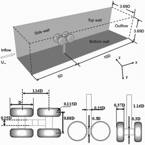
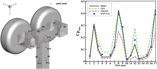
It should be highlighted that the geometry, i.e. Rudimentary Landing Gear, used in this study is a highly-simplified four-wheel landing gear defined by only a few geometric components, which includes main truck, four wheels and a vertical strut. It was also proposed as a benchmark test case for the European Advanced Turbulence Simulation for Aerodynamic Application Challenges (ATAAC) (Alistair, 2018) project and the AIAA workshop on Benchmark problems for Airframe Noise Computations (BANC) project for unsteady CFD methods validation and aeroacoustic predictions. Its dimensions and test flow conditions have been described in detail in earlier experiments and numerical studies (Spalart & Mejia, 2011; Venkatakrishnan et al., 2011). Tested in the low speed wind tunnel at the National Aerospace Laboratories (NAL), Bangalore, India, the RLG model was mounted inversely at the center of the tunnel with wheels facing the flow at zero degree azimuth incidence. The test section here consists of a square cross-section of 3.69Dwidth and 3.69Dheight, which produces a relatively large blockage and decreases the impact of the Reynolds number. The freestream Mach number is , which is equal to an inflow velocity of  m/s. And the diameter of the wheel Dis about 0.406 m, corresponding to a Reynolds number of based on Dand . Data acquired in this experiment include surface oil flow visualization, static surface pressure, static force measurements and unsteady surface pressure. In detail, the unsteady pressures were measured at 36 kulite transducers on the surface of the RLG. Nineteen kulites were distributed along the meridian of the forward wheel, while the rest were positioned on the truck and strut. By rotating the wheel in 2increments about its axis, then measurements can be gathered to obtain a complete pressure map on the wheel. After the wheel completed a rotation of 360, the whole model was rotated in 180so that the measurements on the backward wheel could be gathered. The data of each kulite was sampled at 10 kHz for a total 204,800 pressure measurements. The experimental results were provided by Venkatakrishnan et al. (2011) for code validation and performance assessment.

2.1. Geometry and boundary condition

The computational domain used in this simulation takes the same form as the test section in the wind tunnel at NAL, as shown in Figure 1. In order to capture the pressure fluctuations on the surface of the RLG accurately, compressible effects are taken into account and therefore the air is modeled as an ideal gas. The inlet which is upstream of the center of the landing gear is specified by uniform total pressure boundary condition targeting at  m/s. The pressure outlet condition is set downstream of the center. The reference pressure in the outlet is set to 1 atm and the inlet air temperature is 299 K. The no-slip wall condition and the defaulted adiabatic condition are set for the surface of the RLG model. In addition, the pressure gradients at the wind-tunnel walls are checked against experiment (not shown in this paper) and are weak enough except for the cases at the bottom wall, where a horseshoe vortex is induced due to the presence of the strut. It would be better, as Spalart and Mejia (2011) recommend, to treat all the wind-tunnel walls (the top, side and bottom walls) as inviscid with a slip wall condition such that the boundary layers are not resolved in the computation. However, it would not be accurate to specify the bottom wall as an inviscid wall, and the pressure fluctuations on the bottom wall may not match well with experiment.

Figure 1. Computational domain and dimensions of RLG model (Xiao et al., 2013).

2.2. Computational grid

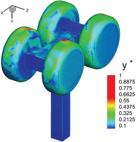
Two sets of multi-block structured grid, the coarse and the fine, are generated using the commercial software POINTWISE for the calculations and the grid sensitivity study. The coarse grid is achieved by decreasing the fine grid points in the x-, y- and z-directions by 40%, respectively, and the overall size of the grid is about 6 million cells for the coarse grid and 14 million for the fine one, as shown in Figures 2(a) and 2(b). Both grids are generated to have a thin wall-surrounding layer around the landing gear walls to capture the boundary layer. The grid spacing in the first layer normal to the wall is about , ensuring that the in the wall-adjacent cell is of the order of unity (Figure 3).

Figure 2. Grids in the x–z-plane with Y=0.

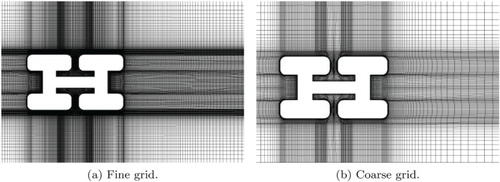
Figure 3. iso-contour over the entire RLG model.

In the fine grid, the grid size on the wheels, truck and strut is about 0.01D, and the grid cells outside the boundary layer are essentially isotropic within a region of away from the landing gear surface. The streamwise grid scales at from the center of the RLG are about 0.035D, which then extend to the outlet at a stretching rate of 1.1.

3. Numerical methods and turbulence modelling

In the present study, all CFD simulations are performed by using the commercial package CFX 14.0 developed by ANSYS, which is based on a discretization of the governing equations using an element-based finite volume method and a pressure–velocity coupled approach. In order to predict the massively separated flow past the RLG accurately, a compressible solver was used and three different kinds of method were applied with all default settings given in the software, including URANS, DDES and the LES dynamic model from Lilly (1992). In both the URANS and DDES approaches, the two-equation k–ωshear stress transport (SST) model developed by Menter (1994) was involved. Based on the earlier k–ωmodel of Wilcox (1988), this model introduced a modification to the eddy viscosity that accounted for the transport of the turbulent shear stress. Not only can this model offer a much more robust and accurate viscous sublayer formulation, but it also produces more accuracy for boundary layers in adverse pressure gradients. Details of the DDES and LES models are given in the following section.

3.1. Delayed detached eddy simulation

The earlier version of DDES developed by Menter and Kuntz (2004) was used in the current simulation. Since the DES methods can be constructed through modification of the destruction term of the turbulent kinetic energy transport equation (Strelets, 2001), the k-equation in DDES can be given by (1) where denotes the turbulent viscosity. The production term and the destruction term are given by (2a) (2b) Differing from the DES-SST proposed by Strelets (2001), the hybrid length scale for DDES can be defined as (3) This length scale can switch between the turbulence length scale and the filter length scale , which are defined as (4a) (4b) where is related to the maximum local mesh spacing as the filter width and denote constants of the original Wilcox model (Wilcox, 1988). is a damping parameter taking the form in the SST model (Strelets, 2001), which offers the highest level of protection against grid induced separation. For example, in the near-wall region with large adverse pressure gradients, equals one and forces the simulation to RANS mode, whereas outside the boundary layer, it turns to zero and switches the mode to LES form.

3.2. Large eddy simulation

For the large eddy simulation, it is critical to employ a subgrid model to account for the physical effects of the unresolved turbulence on the resolved turbulence. In general, the Smagorinsky model (Smagorinsky, 1963) is the most popular subgrid model and provides the eddy viscosity as (5a) (5b) where the carets represent grid-filtering and is the Smagorinsky constant. In this work, for LES is taken as the cubic root of the cell volume. Additionally, the dynamic Smagorinsky–Lilly model is employed and is not taken as a constant any more, but dynamically evaluated for each cell during time-processing following a method proposed by Germano et al. (1991).

3.3. Numerical methods

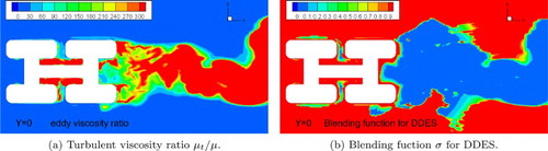
The available ‘high resolution’ scheme of CFX (HRS), which is a bounded second-order upwind biased discretization (ANSYS, 2012), is applied in all the simulations to approximate the convective fluxes in the current work. Based on an approach similar to those of Barth and Jespersen (1989) and Darwish and Moukalled  (2010), this scheme varies between second-order and first-order depending on spatial gradients by calculating the bounded values. This means that, in regions with low variable gradients, a second-order upwind scheme is used, while in areas where the gradients change sharply, a first-order upwind scheme is used to maintain robustness. In particular, for the numerical treatment of DDES, a special built-in mechanism can be activated automatically via the blending function as proposed by Strelets (2001) that allows the use of the HRS in RANS regions and a second-order Central Difference Scheme (CDS) in unsteady regions, i.e. the LES regions. This switch is based again on the hybrid DDES nature and uses the following approximation of the inviscid flux in the governing equations: (6) where and denote the central and the high-resolution approximations of inviscid flux, respectively; σis a blending function (varying from zero to one) which is based on several parameters, including the grid spacing and the ratio of vorticity to strain rate. Figures 4(a) and 4(b) give a clear idea of the performance of the suggested approximation. In the vortical areas of the cavity and the wake of the RLG, where DDES performs in LES mode, σis close to zero and the scheme acts virtually as CDS. On the other hand, in the near-wall RANS regions and the irrotational areas of the flow, σis nearly unity and the scheme is effectively the high-resolution one. As a consequence, the DDES cases in this study could not only benefit from CDS to insure a minimum level of numerical dissipation, but also maintain robustness to prevent near-wall numerical instabilities by using HRS. Thus, the hybrid HRS/CDS scheme of DDES calculations seems to provide low enough numerical dissipation compared with the cases of LES and URANS, which use only HRS.

Figure 4. Distribution of the turbulent viscosity ratio and the blending function for DDES with Y= 0.

In addition, the implicit second-order backward Euler scheme is used for the unsteady formulation in all calculations. Given that the unsteady pressure data is sampled at 10 kHz for each kulite transducer in the experiment (Venkatakrishnan et al., 2011), the same time step, i.e. 0.0001 s, is applied and the total computational time is 1.0 s. On the grounds of the fully implicit solution, only six sub-iterations within each time step are enough to make sure the root mean square (r.m.s.) residual is less than for the convergence criterion to start the next time step. Before the time-averaging process begins, a settle time of 0.2 s is simulated to reach a statistical steady state, then a time sequence of 0.8 s is collected to create a time-averaged data sample.

4. Results and discussion

4.1. Effect of grid resolution

The results of the grid sensitivity study for DDES are plotted in Figures 5–7. Figure 5presents the corresponding non-dimensional vorticity at two planes, across the strut and the truck, respectively. The comparisons clearly show that the effects of the grid density can exert a significant influence on the instantaneous vorticity distribution. The coarse grid presents relatively large-scale structures and a low-resolution flow field. However, the fine grid presents plenty of small-scale structures and the resolution is also higher due to its dense grid scale distribution. Figures 6and 7, respectively, show comparisons of the averaged pressure and the fluctuant pressure between the coarse and the fine grid simulations. The experimental data, labeled EXP NAL, is taken from the ATAAC project website (Alistair, 2018). Here, the pressure coefficient is plotted along the circumferential direction in the center plane of the wheels, and Figure 8(a) clearly displays the azimuthal distribution around the wheels. It is observed that the agreement with measurements between both grids on the averaged pressure is reasonably good, although both of them somewhat underpredict the pressure at 0–of the rear wheel. However, as shown in Figure 7, the coarse grid performs poorly and underpredicts the r.m.s. fluctuant pressure at most locations where flow separation and reattachment can happen regularly. The calculations of the fine grid are in better agreement with the experimental data, indicating that the refinement of the grid has a large impact on the fluctuant field but a negligible influence on the averaged field. Hence, subsequent work will be based only on the fine grid, unless otherwise stated.

Figure 5. Effects of grid density: comparisons are made between the fine grid (left) and the coarse grid (right) through instantaneous vorticity at two sections. The vorticity has been normalized by the diameter of the wheels Dand the freestream velocity .

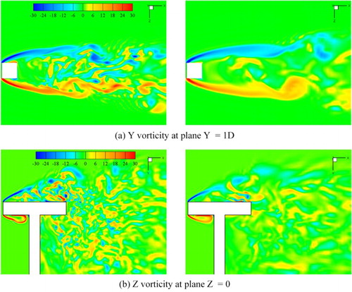
Figure 6. Time-averaged pressure coefficient along the circumference of wheels in different grid densities, centerline with Z=0.440D.

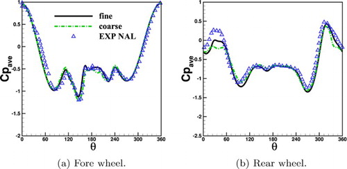
Figure 7. Fluctuant pressure coefficient along the circumference of wheels in different grid densities, centerline with Z=0.440D.

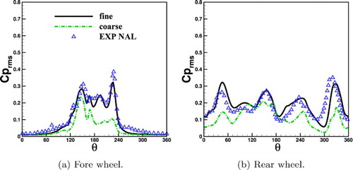
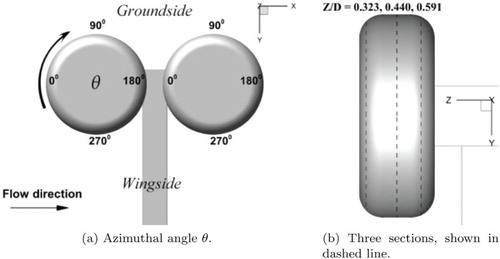
Figure 8. Definition of θand the positions of the three sections along the wheels.

4.2. Comparison of the results obtained with DDES, LES and URANS

In this section, some of the most significant flow features computed are presented and discussed compared with the experimental data in as much detail as possible, with the aim of assessing the performance and viability of different numerical methods in predicting the massively separated flow past the RLG. Unsteady surface SPL and pressure spectra are also validated and discussed afterwards to describe the noise generation.

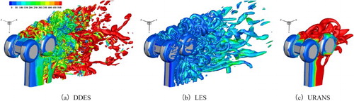
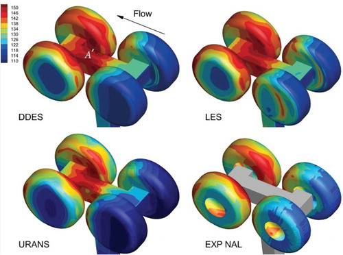
In the following, coherent tridimensional vortices around the RLG are firstly identified by means of the turbulent viscosity ratio as well as the Q-criterion (Hunt, Wray, & Moin, 1988). The iso-surface in Figure 9shows that both DDES and LES can capture abundant vortical structures with the same grid, while DDES seems to resolve smaller vortices, especially between the wheels and in the wake where large-scale vortices decay into smaller ones. This decay is indicated by the higher values of the turbulent viscosity downstream. The main reason for this difference between DDES and LES is probably due to the different definitions of eddy viscosity and the effects of numerical dissipation. For example, in the LES mode of the DDES prediction, it is well known that the assumption of local equilibrium between the production term and the destruction term can lead to the already known relation (7) which means that the eddy viscosity is proportional to the magnitude of the strain tensor and to the square of the filter width (Strelets, 2001), which is very similar to the relation given in Equation (5a(5a) ). As mentioned previously, the filter width for DDES is based on the maximum local mesh spacing, whereas LES uses the cube root of the local cell volume. Hence, DDES can generate a higher level of eddy viscosity than LES can. Consistent with previous explanation, the low dissipative discretization of the convective terms of DDES calculations is sufficient to further resolve smaller scales of motions in the wake compared with those of LES, and a similar phenomenon was also found in the work of Constantinescu and Squires (2003) as the hybrid upwind/central schemes used in DES actually resolve the vortex shedding in the detached shear layers reasonably well. Unfortunately, the result of URANS only shows relatively large structures with the highest eddy viscosity values near walls, leading to higher dissipation of the small flow structures in the wake.

Figure 9. Instantaneous iso-surface of , colored with the turbulent viscosity ratio .

4.2.1. Mean flow patterns in space

Figures 10and 11show the mean flow patterns around the RLG model for two planes through the sections Y=0 and Z=0.44D, respectively. The mean flow fields are generally similar for all the numerical calculations. As shown in Figure 10, all the plots show that the flow separates from the back and the lateral side of the fore wheel, then impinges on the truck and the frontal side of the rear wheel. Behind the rear wheels, a large recirculation zone can be observed, though its shape and extension are slightly different from each other. It should be noted that the flow patterns and the contours in Figure 10are nearly symmetric about the model, ensuring that all the simulations have been run for a sufficient time in both the flow development and the time-averaged process. Distinguishably, all of them indicate several vortices inside the cavity (shown in the dashed rectangle), though the ones simulated by LES are a little larger. What's more, the absence of the separation bubble emanating from the outboard edge at the back of the fore wheel is also remarkable in the results of URANS.

Figure 10. Mean velocity contours with streamlines on the X–Z-plane at Y=0.

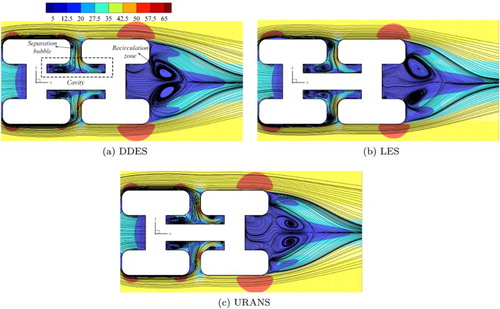
Figure 11. Mean velocity contours with streamlines on the X–Y-plane at Z=0.44D.

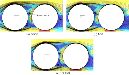
On the circumferential plane (z=0.44D) shown in Figure 11, all the calculations have claimed flow separation behind the fore wheel with approximately similar locations, although different cases show a different separation intensity, and a spiral vortex originating from the fore wheel can easily be seen in the cases of DDES and LES, which indicates the complex flow features between the wheels.

4.2.2. Surface flow patterns and the time-averaged pressure

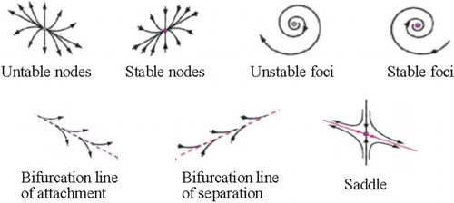
Comparisons of the surface flow patterns as well as the surface averaged pressure distribution on the RLG model are presented in Figures 12–15. Photos of the surface oil flows together with contours of the experimental are also provided. To simplify the description of the complex flow on the wall, the critical points theory proposed by Perry and Chong (1987) is introduced. According to the study of Lazos (2002b) on the surface topology of landing gears, the critical points in this section can be classified into seven groups (shown in Figure 16). Typical patterns presented include UnStable Node (USN), Stable Node (SN), Unstable Foci (UF), Stable Foci (SF), Bifurcation Line of Attachment (BLA), Bifurcation Line of Separation (BLS) and Saddle (S).

Figure 12. Comparisons of surface streamlines and averaged pressure on the wheels, outboard view from front.

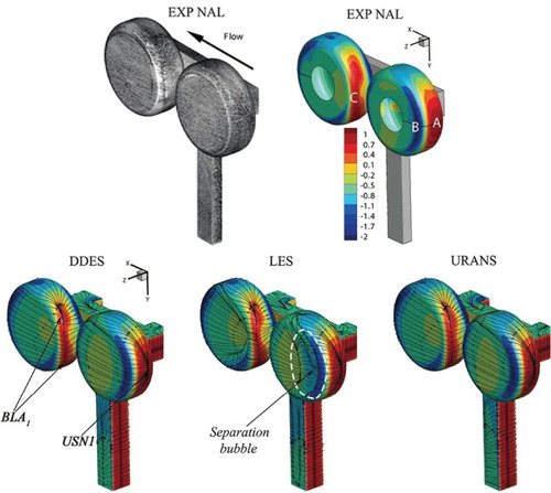
Figure 13. Comparisons of surface streamlines and on the wheels, inboard view.

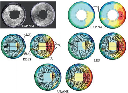
Figure 14. Surface streamlines and on fore wheel, windward view.

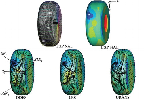
Figure 15. Surface streamlines and on rear wheel, leeward view.

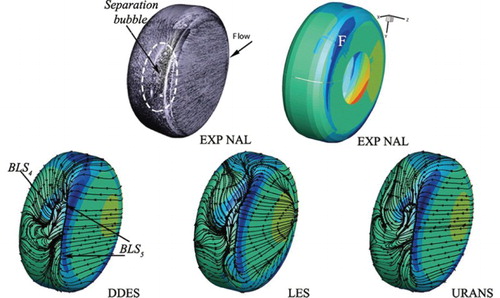
Figure 16. Classification of critical points on surface.

From the front view, shown in Figure 12, the streamlines and pressure coefficients of the attached flow for the three cases are in good agreement with the measurements on the windward side of the wheels. The high-pressure region A corresponds to the stagnation point USN, while C corresponds to the line of attachment BLA, which may probably be ascribed to the impingement of the wake off the fore wheel. However, the flow predicted by LES exhibits a large difference from the experimental and other numerical cases on the lateral sides of both the fore and the rear wheels. With the streamlines converging around the shoulder of the wheels, LES predicts a redundant separation bubble downstream the low-pressure region B. A similar phenomenon was also found in the work of Krajnović et al. (2008), which suggested that this problem might be caused by inaccurate near-wall grid resolution.

Figure 13presents the surface streamlines on the inboard side. Due to the blockage of the rectangular truck, a symmetrical high-pressure region labeled D together with a crescent-shaped separation line BLScan easily be observed on the inboard side of the fore wheel, which indicates a large flow separation. Then parts of the separated flow reattach on the windward side, leading to a line of attachment BLAand a saddle S. The results of DDES and LES match the measurements well, while URANS fails to predict the line of attachment. The other line of separation BLS, which is nearly asymmetric, can be observed on the rear wheel. This can result from the downwash effect of the flow coming off the fore wheel and the vertical strut on the wing side which acts as a blockage. Because of the large flow separation downstream of the rear wheel, little difference can be found among all the flow patterns, while DDES shows better agreement with the measurements in the shape of pressure contours.

The rear view of the fore wheel in Figure 14shows the complicated nature of the flow. A stable focus SFis formed by the high-speed fluid from the ground side and the inboard side of the wheel, which leads to strongly unsteady behaviors like vortex shedding indicated by the formation of the low-pressure region E (Venkatakrishnan et al., 2011). The majority of the flow separates off the edge on the shoulder (labeled BLS) and then impinges on the rear wheel. The rest reattaches on the fore wheel and forms the saddle at where it meets the flow forming the focus. On the wing side, a stagnated region characterized by the unstable node USNcan be observed (Venkatakrishnan et al., 2011), which might be caused by separated flow reattachment on the wing side. Compared against the experimental data, all the simulations match the oil flow measurements well on the ground side and the difference is trivial, while DDES shows better agreement in the shape of pressure contours and the position of the saddle (164, 162 and for DDES, LES and URANS, respectively). Only DDES captures the unstable node on the windward side at , though the predicted position is slightly different from the measurements (at ), which indicates the superiority of DDES in predicting small-scale flow separation and reattachment.

From the rear view of the back wheel, shown in Figure 15, the flow patterns are relatively simpler than those on the fore wheel in Figure 14. The high-speed fluid from the ground side converges and separates forming the line of separation BLSwhere it meets the separated flow from the outboard side forming a large separation bubble. The line of separation shown as BLScan be found on the outboard side in which the low-pressure region F is located. Characterized by massive flow separation, a large low-velocity region on the wing side can be observed indicated by the higher pressure level, and the computational pressure contours look similar to those in experiments, although all the numerical calculations predict a somewhat larger region F.

Comparisons of the coefficients of the wheels are also presented quantitatively in Figures 17and 18at three sections in the z-direction, and their positions have already been shown in Figure 8(b).

Figure 17. Distribution of of three sections on the fore wheel using DDES, LES and URANS.

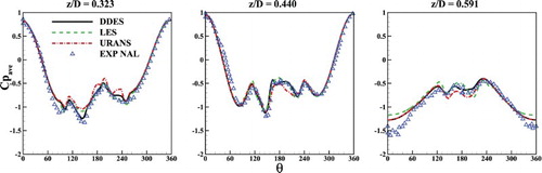
Figure 18. Distribution of of three sections on the rear wheel using DDES, LES and URANS.

The computed and experimental surface distributions for the fore wheel are shown in Figure 17along the circumferential direction. In general, the agreement between the values of the experiment and the three numerical cases is quite good. All of them can predict the pressure at the attached regions on the windward side well. However, a relatively obvious difference can be found on the outboard side (z=0.591D) where the low-pressure region B exists (and ), almost all the calculations overpredict the . The main discrepancies occur particularly in the valley () of the curve on the inboard side (z=0.323D). This directly corresponds to the low-pressure region E where amounts of separation and vortex shedding may happen. But the calculations of DDES show the best agreement with the measurements while others predict slightly higher pressure values.

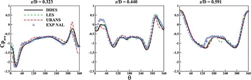
On the rear wheel shown in Figure 18, the trends of ups and downs in these graphics are totally different from those on the fore wheel – in particular for on the inboard side, where a trough of can be seen. This suggests that a small low-pressure region is formed on the ground side next to the high-pressure region C. In addition, the crest shown at also indicates the asymmetry of region C, which is mainly caused by the blockage effect of the vertical strut. At the position for in the three plots, all the calculations predict a gentle pressure plateau which indicates a large flow separation on the leeward side of the rear wheel, and the agreement with the measurements is good except for that of LES on the outboard side. The reason for this is not clear but may again be caused by the poor grid resolution in the near-wall region. On the other hand, the DDES calculations again show the best agreement with the measurements. LES has a slightly poorer performance when predicting the flow around the shoulder on the outboard side where the flow is full of turbulence. Another notable aspect from these plots is that URANS has difficulty in matching the measurements on the high-pressure region C where flow reattachment and impingement occur recurrently. In spite of these differences observed in the predicted magnitude, all the calculations suggest similar tendencies for and are consistent with the experimental data.

4.2.3. Pressure lift and drag coefficients

In this subsection, the computational pressures are integrated over the surface of the wheels and averaged during the calculation to give the averaged pressure lift and drag coefficients in Table 1. The reference area here is taken as (Xiao et al., 2010), which is the sum of the frontal projected area of the whole RLG model. All the simulations produce a credible drag coefficient with a maximum 2.5% difference from the experimental data of Spalart and Mejia (2011). However, the prediction of the lift force coefficients is poor, and the discrepancy is more than 60% of the experimental measurement. Similar results can be found from other research groups using DES and LES in Spalart and Mejia (2011). Almost all the CFD results are higher than experiment, and the reason is still unknown. Turning to the predicted root-mean-square values of the lift and drag coefficients (and ), the calculations of DDES and LES yield quite similar predictions, while those of URANS yield the lowest ones. Meanwhile, Figure 19shows the PSD of the computational drag coefficient. It is interesting to note that the Strouhal number (St) is not particularly sensitive to the choice of simulation approach, since all the calculations yield a primary frequency where St is about 1.0. However, URANS presents a slightly lower PSD level than DDES and LES even if they obtain similar trends for ups and downs, which shows the poor performance of URANS in capturing fluctuations.

Figure 19. Power spectral density of using different methods.

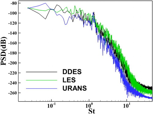
Table 1. Comparisons of force coefficients for the whole RLG model.

EXP	1.600	−0.650	–	–
DDES	1.612	−0.234	0.0421	0.0602
LES	1.641	−0.194	0.0433	0.0665
URANS	1.596	−0.248	0.0280	0.0298

Forces on entire model from Spalart and Mejia (2011).

The results for a wheel-by-wheel comparison are shown in Table 2. As expected, the predicted drag coefficients for wheels are again in quite close agreement with the measurements, and little difference can be found between the results of DDES and LES. Relatively, URANS appears to underestimate of the rear wheel by 16.5%. However, the results for lift coefficients are more encouraging than those in Table 1. The difference from the measurements is acceptable, and it is less than 0.01 for wheels when DDES is employed. The reason for this is unknown but might probably lie in the inappropriate pressure distribution on the truck and strut or the inviscid wind-tunnel wall condition on the windward side.

Table 2. Comparisons of force coefficients for the wheels.

	Fore	Rear	Fore	Rear
EXP	0.240	0.170	−0.050	−0.030
DDES	0.232	0.160	−0.058	−0.022
LES	0.233	0.161	−0.045	−0.026
URANS	0.240	0.143	−0.058	−0.026

Results for wheels from Spalart and Mejia (2011).

4.2.4. Unsteady on-surface pressure

To explore the region with potential noise generation, the unsteady surface pressure fluctuations on the RLG model are compared with the existing experimental data collected by kulite unsteady pressure sensors. Figure 20presents an overview of the whole RLG model with the SPL distributions, into which the r.m.s. pressure fluctuations are transformed. Both DDES and URANS calculations show much lower values of SPL than those of the experiment (about 10 dB) in the first half part of the fore wheels. As expected, this discrepancy is reasonable since the flow behaves in an attached manner and both DDES and URANS behave in RANS mode in the region. On the other hand, LES presents higher SPL values on the lateral side where non-physical flow separation happens. With the fluid moving rearward, the flow becomes more unsteady and turbulent, and the SPL values appear to be higher at the back of the fore wheels where flow separation and vortex shedding happen regularly.

Figure 20. Distribution of the surface SPL on the ground side of the RLG model.

Owing to the impingement of the separated shear flow off the fore wheels, several large high-SPL regions colored in red are generally identified on the ground-facing surface of the truck (i.e. ) and the inner-front side of the rear wheels in all the simulations. In these regions, especially in where the maximum SPL could reach above 150 dB, extensive vortex motions like vortex shedding, sweeping and interactions have been confirmed by the animations (not shown in this paper), and the SPL patterns around are quite similar between the calculations of DDES and LES. URANS on the other hand shows a slightly smaller shape of , and the values of SPL are a bit lower, too. What's more, the total level of the SPL obtained by URANS is comparatively low. Only in the region where large-scale flow separation happens directly can it provide reliable results, showing the poor capacity of URANS to capture the pressure fluctuations due to its large numerical dissipation downstream of the wheels.

However, because of the lack of kulite transducers, the contours of SPL for EXP NAL cannot be mapped on the truck and strut. Instead, the comparisons of at 15 sample points on the truck and strut are presented in Figure 21. The computational results of DDES are in best agreement with the measurements, except at point 12 where a large discrepancy of about 0.035 occurs on the wing side of the truck. In contrast, LES produces much higher values at point 12 and the difference reaches about 0.1. LES also predicts higher values at points 4 and 16 on the strut while URANS predicts the lowest values at all of these positions. That difference is possibly caused by shear-layer instability from the sharp edge, which seems to be predicted too upstream by LES but a bit downstream by DDES. Nonetheless, both DDES and LES can predict the pressure fluctuations well at points 2 and 9, between which the high-SPL region is located.

Figure 21. Comparisons of at the 15 sample positions on the truck and strut.

The details of SPL on the wheels are compared between Figures 22and 23in order to discuss further the rest of the high-SPL regions, and the extrema of SPL over the wheels are also presented in Table 3separately.

Figure 22. Comparisons of the high-SPL regions on the fore wheel.

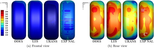
Figure 23. Comparisons of the high-SPL regions on the rear wheel.

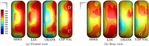
Table 3. Comparisons of SPL extrema over the wheels.

	SPL(dB)		SPL(dB)
	Fore	Rear	Fore	Rear
EXP	112	121	147	151
EXP NAL	117	121	144	149
DDES	107	119	144	150
LES	110	121	145	150
URANS	100	113	143	147

Results for wheels from Spalart and Mejia (2011).

On the forward surface of the front wheel, which is shown in Figure 22, the disagreement with experiment is obvious but foreseeable as both DDES and URANS act in RANS mode in the attached region. LES provides a slightly higher SPL (about 3 dB on average) in this region, but it is still too large for aeroacoustic prediction. On the rearward surface, the difference between computations and measurements is relatively smaller while the calculations of DDES show better agreement with the experimental data. Two high-SPL regions labeled Band Ccan be clearly observed in the simulations of DDES and LES. Both of them can reach the maximum SPL value at 144 dB. However, LES provides larger shapes of these regions and higher SPL extrema (about 145 dB). The main reason might be that the non-physical separation produced by LES can have an unneglectable impact on the prediction of fluctuations. In addition, the region Boften corresponds to vortex shedding as well as the focus shown in Figure 14, while Ccorresponds to unsteady separations and reattachment. As expected, URANS gets the worst results and cannot offer reasonable SPL values in the high-SPL regions.

On the rear wheel presented in Figure 23, two main noise sources can be identified on the inboard side of the windward surface where turbulent wakes from the fore wheels impinge. One with very high-SPL value (region D, about 149 dB) is on the ground side while the other with relatively high-SPL value (region E, about 147 dB) is on the windward side. The agreement between the computations and the measurements is similar to that observed on the fore wheel. DDES presents more suitable shapes and distributions while those predicted by LES are a little larger. In addition, both of them overpredict the SPL extrema in region Dby about 1 dB. URANS once again provides smaller scope and lower extrema (about 147 dB) in regions Dand E. On the leeward surface, another two high-SPL regions, Fand G, can be observed, which might be caused by the massively unsteady separation. However, the results of all the simulations match the measurements less satisfactorily, and even the DDES calculations struggle to provide reasonable shapes and extension for these regions. In this regard, extensive work remains to be done.

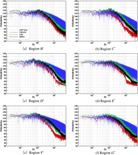
Seeking more quantitative validation, six selected locations near the high-SPL regions are chosen to compare computational results with the experimental unsteady pressure signals. It should be noted that the experimental data are sampled at 10 kHz for about 20 seconds for a total of 204,800 pressure measurements. Following the same sampling frequency, the computational results are collected for 0.8 s for about 8000 measurements. The frequency resolution is about 0.07 and 2 Hz for experimental and computational measurements, respectively. Figure 24compares the experimental and numerical PSD levels in decibels versus Strouhal number () at six high-SPL locations from Bto G. In general, both DDES and LES can predict the pressure fluctuations well at low frequencies for . However, LES presents a slightly higher PSD than DDES at G, which is consistent with the comparisons shown in Figure 23. URANS shows similar trends of ups and downs at low frequencies, but the overall SPL levels are slightly lower than those in other calculations and measurements, especially at the location of C. In addition, both DDES and LES together with URANS capture an obvious primary frequency at B, Cand D, where St is around 1.0. This demonstrates that the flow separates and reattaches periodically from the front wheel. At high frequencies where St is above 10, all of the three calculations significantly underestimate the levels of PSD, especially in the case of URANS, which yields the lowest levels and struggles to predict the pressure fluctuations at high frequencies. It should also be noted that this frequency cut-off might be caused by the grid resolution combined with the numerical dissipation, and the small-scale structures captured by DDES and LES might not be acousticallysufficient.

Figure 24. Comparison of Power Spectral Density (PSD) for sampling surface pressures at six locations of the high-SPL regions from Bto G.

4.2.5. Total Turbulent Kinetic Energy (TKE)

High-order statistics of all the simulations are also shown in Figure 25by contours of the resolved turbulent kinetic energy , which is non-dimensionalized by the square of the freestream velocity. For all cases, a high level of the resolved flow-field unsteadiness can be found in the vicinity of the region , where the TKE peaks at values of about 0.303, 0.309 and 0.255 for DDES, LES and URANS, respectively. Downstream of the RLG model, the entire wake region is also energetic for both DDES and LES. However, the large deviation between the DDES and LES calculations is that the shear layer originating from the wing side of the truck's leading edge as well as the wake of the vertical strut is not equally well captured. 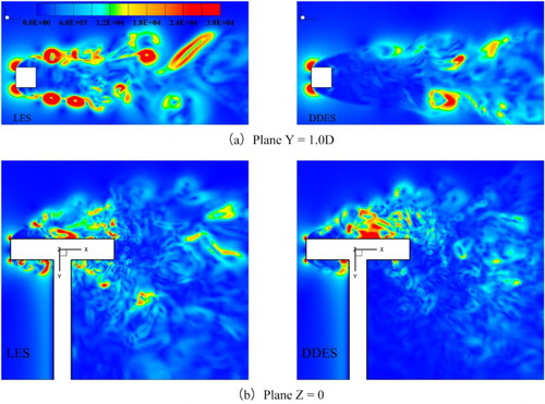In the case of LES, the energetic region behind the strut seems to be somewhat more upstream, which happens at about , with that of DDES happening at 1.5D, and the shear layer separating from the sharp edge of the truck (shown in the dashed rectangle) is more turbulent with a peak value of TKE at 0.13, while that of DDES only reaches 0.06. However, this might reflect the Kelvin–Helmholtz (K-H) instability in these separated shear layers at such Reynolds numbers. Figure 26presents some K-H like structures which are visualized by the instantaneous magnitude of pressure gradient using DDES and LES. Qualitatively speaking, since reasonable structures and unsteadiness are detected behind the strut and on the wing side of the truck, it is possible for LES to detect the K-H instability occurring in the shear layers and leading to transition. Such detailed flow structures are not resolved by the DDES simulation, as shown in Figure 26(a). Therefore, DDES may fail to resolve the K-H instability, although the same grid is applied in both cases. As mentioned in the previous study in Figure 21, LES is still unable to resolve the exact position where K-H instability starts to occur. Instead, it always gives an earlier prediction, which is probably due to inadequate near-wall grid resolution. On the other hand, the weakness of TKE in URANS is particularly evident downstream of the wheels where turbulent fluctuations don't persist, and no shear layer instability is detected by URANS (not shown in this paper).

Figure 25. Distributions of dimensionless resolved TKE in the X–Y-plane, Z= 0.

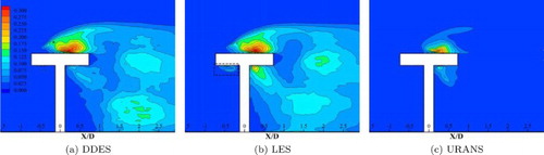
Figure 26. Visualization of the instantaneous magnitude of pressure gradient in both calculations of DDES (right) and LES (left) at two planes, (a) plane Y=1.0D; (b) plane .

4.3. Generation of the main noise sources

To identify the dominant noise sources and reveal the relevant physical mechanisms responsible for noise generation, one way is to obtain an in-depth understanding of the noise generation mechanism by linking the simultaneous visualizations of the instantaneous flow and the sound pressure field. In this subsection, the SPL distribution together with the instantaneous vorticity, which is normalized by the diameter of the wheels Dand freestream velocity , is presented to show the generation of the very-high SPL regions , Dand Eusing DDES. Figure 27depicts the transient evolutionary process of the instantaneous vorticity between the wheels at different sections, respectively. The vortical features on the X–Z-plane through Cand Eare shown in Figure 27(a). Here, DDES clearly displays the transient vortex evolution (shown in the dashed rectangles) from the fore wheel, including the birth development (1), formation of the elongation (2), rupture, shedding (3) and impingement (4) onto the outward part of the rear wheel. Meanwhile, the shear layers generated from the sharp corner of the strut also join the impingement, although onto the inner side of the rear wheel, and these strongly periodic behaviors commonly lead to high SPL of the wide-ranging region E.

Figure 27. Distribution of the Yvorticity on two different X–Z-planes, with the surface contours colored by SPL, viewed from the wing side (a) and the ground side (b). Only about half of the model is given and the contour legends of SPL are no longer provided.

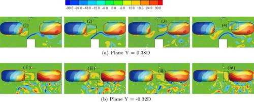
On the ground side of the wheels, the cut plane through regions Band D, where SPL peaks at 144 and 149 dB on the fore wheel and rear wheel, respectively, is presented in Figure 27(b). In the absence of the vertical strut, the alleviation of the blockage effect is evident from the fact that the shear layers detached from the leading edge of the truck, destabilize and break down into small pieces. Hence the vortical structures shown here are more abundant than those on the wing side. On the other hand, it can be observed that the vortex shed from the fore wheel has a significant effect on its surrounding eddies and region D. The vortex (shown in the dashed rectangles) is born near Band immediately swirls downstream in a clockwise direction (i), then it evolves and ruptures (ii), and impinges partly on D(iii). Afterwards, the rest of the vortices combine with each other and eventually impinge on the windward surface (iv) of the rear wheel. It should be noted that the vortex motions and interactions between the wheels are so strong that even the surrounding vortices detached from the truck can spiral into this area. These are probably the main reasons why the SPL at Dcan reach its highest on the rear wheel.

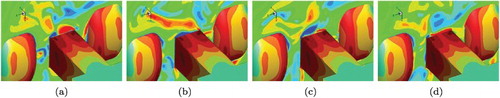
On the ground side of the sharp corner regions, Figures 28(a)–28(d) show strong interactions between vortices and the sharp square edge. The very-high SPL region , where the maximum of SPL is over 150 dB, can be generally understood as a consequence of the alternate vortex shedding that happens periodically on both sides of the sharp corner of the truck. It is interesting to note that the vortex shed from one side particularly spirals upward to the opposite side, showing that the strongly mutual interactions between vortices also exist around .

Figure 28. Distribution of the Xvorticity on the Y–Z-plane, , with the surface contours colored by SPL, viewed from the ground side of the truck.

5. Conclusion

Based on the industrial software ANSYS-CFX, the unsteady flow around the rudimentary landing gear placed in a wind tunnel has been investigated by the two-equation DDES-SST and URANS-SST models as well as the LES dynamic model. Two sets of grids with 6 million and 14 million grid points were employed to explore the effects of the grid resolution of DDES. The grid sensitivity study demonstrates that the grid density has a negligible impact on the prediction of the mean flow quantities, but has a significant influence on the unsteady pressure fluctuations, and that the finer the grid, the better the agreement with the measurements will be.

Based on the fine grid, a comparative analysis between the computational results of DDES, LES, URANS and the experimental measurements has been conducted to show the physically and geometrically complex flow in as much detail as possible.

1. In the time-averaged computations, URANS shows reasonable prediction in the attached region but is not able to capture the small-scale flow separation and reattachment between the wheels. In general, both DDES and LES with the same grid can agree reasonably well with the experiments in respect of the surface flow patterns and the mean pressure field. However, the near-wall flow structures that are responsible for turbulence are not resolved in LES due to poor near-wall grid resolution. Surprisingly, this results in a non-physical separation bubble on the lateral side of the fore wheel where flow was originally attached, thus showing the great advantage of DDES in predicting the massively separated flow past the RLG in both the attached and separated regions.

2. In the fluctuant and instantaneous simulations, neither LES nor URANS is able to predict the pressure fluctuations accurately on the wheels, truck and the vertical strut. As expected, URANS drastically underestimates the SPL on the wheels because of its large numerical dissipation, while LES somewhat overpredicts it due to the non-physical separation and the premature shear layer instability. DDES, on the other hand, shows better capability in predicting these fluctuations and PSD spectra on the wheels where vortex shedding and impingement happen periodically, indicating its suitability for physical-based noise calculations of landing gears. DDES also resolves smaller and richer flow structures than those by LES.

3. Unfortunately, without enough unsteady experimental data on the truck and strut, we cannot fully ascertain the real positions where the shear layer instability, i.e. transition, occurs. But it seems that the transition predicted by LES is somewhat earlier, while DDES produces a slightly later transition.

Last but not the least, the mechanisms of landing gear noise generation are highlighted in this paper using DDES. The main noise sources on the windward side of the rear wheel marked as Dand Ewith high-SPL values are mainly caused by the strongly periodic impingement of vortex shedding off the leeward side of the fore wheel. On the other hand, intense interactions between vortices and the sharp corner on both sides of the truck and the alternate vortex shedding are evident and are responsible for the formation of the very-high SPL region Aon the truck. What's more, there also exists strongly mutual interference between vortices downstream of the ground side of the fore wheel, where amounts of small-scale vortices are pulled into this large spiral.

It should be noted that the present work mainly studies the flow features and the near-field noise generation of landing gear, and viscous effects of the wind-tunnel walls are not considered. Future work will mainly focus on the far-field noise prediction and noise reduction methods of landing gear, and the simulated cases will be closer to real conditions, such as considering the effects of roughness of wind-tunnel walls. Moreover, one shortcoming of this research may lie in the inappropriate spatial–temporal resolution of the simulation, since the two grids under consideration may not be acoustically sufficient to resolve higher frequencies, and further mesh refinement is desirable. Furthermore, the effects of different time steps will also be studied in the next step, and refinement of the temporal resolution will be included.

Acknowledgements

The authors would like to acknowledge the use of the computing services of the High Performance Computing Center of Northwestern Polytechnical University.

Disclosure statement

No potential conflict of interest was reported by the authors.

Additional information

Funding

This work was partially supported by the National Natural Science Foundation of China [Grant No. 11472223]; the Aeronautical Science Foundation of China [Grant No. 2016ZA53008]; the Fundamental Research Funds for the Central Universities of China; the Seed Foundation of Innovation and Creation for Graduate Students in Northwestern Polytechnical University [ZZ2018050]; the 111 Project [B17037]; and the ATCFD Project [2015-F-016].

References

- Alistair, R.(2018, June 18). Advanced turbulence simulation for aerodynamic application challenges: A seventh framework project [Experimental data on Boeing landing gear]. Retrieved from http://cfd.mace.manchester.ac.uk/twiki/bin/view/ATAAC/TestCase012SimpleLandingGear
- ANSYS(2012). ANSYS user manual CFX-solver theory guide. Canonsburg, PA: ANSYS.
- Ardabili, F. S., Najafi, B., Shamshirband, S., Minaei Bidgoli, B., Deo, R. C., & Chau, K.-w.(2018). Computational intelligence approach for modeling hydrogen production: A review. Engineering Applications of Computational Fluid Mechanics, 12(1),438–458. doi: 10.1080/19942060.2018.1452296
- Barth, T., & Jespersen, D.(1989, January). The design and application of upwind schemes on unstructured meshes. InProceedings of the 27th aerospace sciences meeting, Reno, NV, AIAA Paper 89-0366. Reston, VA: American Institute of Aeronautics and Astronautics. doi: 10.2514/6.1989-366
- Boorsma, K., Zhang, X., & Molin, N.(2010). Landing gear noise control using perforated fairings. Acta Mechanica Sinica, 26(2), 159–174. doi: 10.1007/s10409-009-0304-0
- Chow, L. C., Mau, K., & Remy, H.(2002, June). Landing gears and high lift devices airframe noise research. In MAERO02. Proceedings of the 8th AIAA/CEAS aeroacoustics conference & exhibit, Breckenridge, CO. AIAA Paper 2002-2408. Reston, VA: American Institute of Aeronautics and Astronautics. doi: 10.2514/6.2002-2408
- Constantinescu, G. S., & Squires, K. D.(2003). LES and DES investigations of turbulent flow over a sphere at Re=10,000. Flow, Turbulence and Combustion, 70(1-4), 267–298. doi: 10.1023/B:APPL.0000004937.34078.71
- Darwish, M. S., & Moukalled, F. (2003). TVD schemes for unstructured grids. International Journal of Heat and Mass Transfer, 46(4), 599–611. doi: 10.1016/S0017-9310(02)00330-7
- Dobrzynski, W.(2010). Almost 40 years of airframe noise research: What did we achieve?Journal of Aircraft, 47(2), 353–367. doi: 10.2514/1.44457
- Fotovatikhah, F., Herrera, M., Shamshirband, S., Chau, K.-w., Faizollahzadeh Ardabili, S., & Piran, M. J.(2018). Survey of computational intelligence as basis to big flood management: Challenges, research directions and future work. EngineeringApplications of Computational Fluid Mechanics, 12(1), 411–437. doi: 10.1080/19942060.2018.1448896
- Germano, M., Piomelli, U., Moin, P., & Cabot, W. H.(1991). A dynamic subgrid-scale eddy viscosity model. Physics of Fluids A: Fluid Dynamics, 3(7), 1760–1765. doi: 10.1063/1.857955
- Guo, Y., Yamamoto, K. J., & Stoker, R. W.(2006). Experimental study on aircraft landing gear noise. Journal of Aircraft, 43(2), 306–317. doi: 10.2514/1.11085
- Hao, A., & Jia, Y.(2016). Numerical investigation of flow control using vertex generator for landing gear noise reduction. In Proceedings of the 22nd AIAA/CEAS aeroacoustics conference, 30 May–1 June 2016, Lyon, France. AIAA Paper 2016-2773. Reston, VA: American Institute of Aeronautics and Astronautics. doi: 10.2514/6.2016-2773
- Hedges, L. S., Travin, A. K., & Spalart, P. R.(2002). Detached-eddy simulations over a simplified landing gear. Journal of Fluids Engineering, 124(2), 413–423. doi: 10.1115/1.1471532
- Hunt, J. C. R., Wray, A. A., & Moin, P.(1988). Eddies, streams, and convergence zones in turbulent flows (Report No. CTR-S88). Center for Turbulence Research, Stanford, CA.
- Karthikeyan, N., & Venkatakrishnan, L.(2011). Application of photogrammetry to surface flow visualization. Experiments in Fluids, 50(3), 689–700. doi: 10.1007/s00348-010-0978-x
- Kennedy, J., Neri, E., & Bennett, G. J.(2016, May). The reduction of main landing gear noise. In Proceedings of the 22nd AIAA/CEAS aeroacoustics conference, Lyon, France. AIAA Paper 2016-2990. Reston, VA: American Institute of Aeronautics and Astronautics. doi: 10.2514/6.2016-2900
- Krajnović, S., Larusson, R., & Basara, B.(2012). Superiority of PANS compared to LES in predicting a rudimentary landing gear flow with affordable meshes. International Journal of Heat and Fluid Flow, 37,109–122. doi: 10.1016/j.ijheatfluidflow.2012.04.013
- Lazos, B. S.(2002a). Mean flow features around the inline wheels of four-wheel landing gear. AIAA Journal, 40(2), 193–198. doi: 10.2514/2.1642
- Lazos, B. S.(2002b). Surface topology on the wheels of a generic four-wheel landing gear. AIAA Journal, 40(12), 2402–2411. doi: 10.2514/2.1608
- Lazos, B. S.(2004). Reynolds stresses around the wheels of a simplified four-wheel landing gear. AIAA Journal, 42(1), 196–198. doi: 10.2514/1.597
- Lilly, D. K.(1992). A proposed modification of the Germano subgrid-scale closure method. Physics of Fluids A: Fluid Dynamics, 4(3), 633–635. doi: 10.1063/1.858280
- Lockard, D., Khorrami, M., & Li, F.(2004, May). High resolution calculation of a simplified landing gear. In Proceedings of the 10th AIAA/CEAS aeroacoustics conference, Manchester, UK. AIAA Paper 2004-2887. Reston, VA: American Institute of Aeronautics and Astronautics. doi: 10.2514/6.2004-2887
- Menter, F. R.(1994). Two-equation eddy-viscosity turbulence models for engineering applications. AIAA Journal, 32(8), 1598–1605. doi: 10.2514/3.12149
- Menter, F. R., & Kuntz, M.(2004). Adaptation of eddy-viscosity turbulence models to unsteady separated flow behind vehicles. In The aerodynamics of heavy vehicles, trucks, buses, and trains(pp. 339–352). Berlin: Springer. doi: 10.1007/978-3-540-44419-0_30
- Monclar, P.(2003, July). Landing gear technology programmes. In Proceedings of the AIAA international air and space symposium and exposition: The next 100 years, Dayton, OH. AIAA Paper 2003-2505. Reston, VA: American Institute of Aeronautics and Astronautics. doi: 10.2514/6.2003-2505
- Mou, B., He, B. J., Zhao, D. X., & Chau, K.(2018). Numerical simulation of the effects of building dimensional variation on wind pressure distribution. Engineering Applications of Computational Fluid Mechanics, 11(1), 293–309. doi: 10.1080/19942060.2017.1281845
- Niu, J., Zhou, D., & Liang, X.(2018). Numerical investigation of the aerodynamic characteristics of high-speed trains of different length under crosswind with or without windbreaks. Engineering Applications of Computational Fluid Mechanics, 12(1), 195–215. doi: 10.1080/19942060.2017.1390786
- Oerlemans, S., & de Bruin, A.(2009, May). Reduction of landing gear noise using an air curtain. In Proceedings of the 15th AIAA/CEAS aeroacoustics conference, Miami, FL. AIAA Paper 2009-3156 (pp. 813–837). Reston, VA: American Institute of Aeronautics and Astronautics. doi: 10.2514/6.2009-3156
- Perry, A. E., & Chong, M. S.(1987). A description of eddying motions and flow patterns using critical-point concepts. Annual Review of Fluid Mechanics, 19(1), 125–155. doi: 10.1146/annurev.fl.19.010187.001013
- Shi, Y., Xu, Y., Zong, K., & Xu, G.(2018). An investigation of coupling ship/rotor flowfield using steady and unsteady rotor methods. Engineering Applications of Computational Fluid Mechanics, 11(1), 417–434. doi: 10.1080/19942060.2017.1308272
- Smagorinsky, J.(1963). General circulation experiments with the primitive equations. Monthly Weather Review, 91(3), 99–164. doi: 10.1175/1520-0493(1963)091<0099:GCEWTP>2.3.CO;2
- Spalart, P. R., Deck, S., Shur, M. L., Squires, K. D., Strelets, M. K., & Travin, A.(2006). A new version of detached-eddy simulation, resistant to ambiguous grid densities. Theoretical and Computational Fluid Dynamics, 20(3), 181. doi: 10.1007/s00162-006-0015-0
- Spalart, P. R., Jou, W. H., Strelets, M., & Allmaras, S. R.(1997, August). Comments on the feasibility of LES for wings, and on a hybrid RANS/LES approach. In Proceedings of the first AFOSR international conference in DNS/LES: Direct numerical simulation and large eddy simulation, Ruston, LA (pp. 137–148). Columbus, OH: Greyden Press. Retrieved from https://www.tib.eu/en/search/id/BLCP%3ACN032430355/Comments-on-the-Feasibility-of-LES-for-Wings-and/
- Spalart, P., & Mejia, K.(2011, January). Analysis of experimental and numerical studies of the rudimentary landing gear. In Proceedings of the the 49th AIAA aerospace sciences meeting including the new horizons forum and aerospace exposition, Orlando, Florida. AIAA Paper 2011-355. Reston, VA: American Institute of Aeronautics and Astronautics. doi: 10.2514/6.2011-355
- Spalart, P., Shur, M., Strelets, M., & Travin, A.(2010). Initial RANS and DDES of a rudimentary landing gear. In LES and DNS of the flow with heat transfer in a rotating cavity(pp. 101–110). Berlin: Springer. doi: 10.1007/978-3-642-14168-3_8
- Spalart, P. R., Shur, M. L., Strelets, M. K., & Travin, A. K.(2011). Initial noise predictions for rudimentary landing gear. Journal of Sound and Vibration, 330(17), 4180–4195. doi: 10.1016/j.jsv.2011.03.012
- Strelets, M.(2001, January). Detached eddy simulation of massively separated flows. In Proceedings of the 39th Aerospace Sciences Meeting and Exhibit, Reno, NV. AIAA Paper 2001-0879). Reston, VA: American Institute of Aeronautics and Astronautics. doi: 10.2514/6.2001-879
- Takaishi, T., Inoue, T., Lee, H.-H., Murayama, M., Yokokawa, Y., Ito, Y., & Yamamoto, K.(2017, June). Noise reduction design for landing gear toward FQUROH flight demonstration. In Proceedings of the 23rd AIAA/CEAS aeroacoustics conference, Denver, CO. AIAA Paper 2017-4033. Reston, VA: American Institute of Aeronautics and Astronautics. doi: 10.2514/6.2017-4033
- Travin, A. K., Shur, M. L., Spalart, P. R., & Strelets, K. M.(2006, September). Improvement of delayed detached-eddy simulation for LES with wall modelling. In ECCOMAS CFD. Proceedings of the European conference on computational fluid dynamics, Delft, The Netherlands. Retrieved from http://www.cobaltcfd.com/pdfs/ECCOMAS_2006_improvement_DDESl.pdf
- Venkatakrishnan, L., Karthikeyan, N., & Mejia, K.(2011). Experimental studies on a rudimentary four wheel landing gear. AIAA Journal, 50(11), 2435–2447. doi: 10.2514/1.J051639
- Wang, L., Mockett, C., Knacke, T., & Thiele, F.(2013, May). Detached-eddy simulation of landing-gear noise. In Proceedings of the 19th AIAA/CEAS aeroacoustics conference, Berlin (pp. 1075–1083). AIAA Paper 2013-2069. Reston, VA: American Institute of Aeronautics and Astronautics. doi: 10.2514/6.2013-2069
- Wilcox, D.(1988). Multiscale model for turbulent flows. AIAA Journal, 50(11), 1311–1320. doi: 10.2514/3.10042
- Xiao, Z., Liu, J., & Fu, S.(2010). Calculations of massive separation around landing-gear-like geometries. Journal of Hydrodynamics, 22(5), 883–888. doi: 10.1016/s1001-6058(10)60054-6
- Xiao, Z., Liu, J., Luo, K., Huang, J., & Fu, S.(2013). Investigation of flows around a rudimentary landing gear with advanced detached-eddy-simulation approaches. AIAA Journal, 51(1), 107–125. doi: 10.2514/1.j051598
- Yokokawa, Y., Imamura, T., Ura, H., Uchida, H., Yamamoto, K., & Kobayashi, H.(2010, June). Experimental study on noise generation of a two-wheel main landing gear. In Proceedings of the 16th AIAA/CEAS aeroacoustics conference, Stockholm. AIAA Paper 2010-3973. Reston, VA: American Institute of Aeronautics and Astronautics. doi: 10.2514/6.2010-3973