Sugarcane growth prediction based on meteorological parameters using extreme learning machine and artificial neural network

ABSTRACT

Management strategies for sustainable sugarcane production need to deal with the increasing complexity and variability of the whole sugar system. Moreover, they need to accommodate the multiple goals of different industry sectors and the wider community. Traditional disciplinary approaches are unable to provide integrated management solutions, and an approach based on whole systems analysis is essential to bring about beneficial change to industry and the community. The application of this approach to water management, environmental management and cane supply management is outlined, where the literature indicates that the application of extreme learning machine (ELM) has never been explored in this realm. Consequently, the leading objective of the current research was set to filling this gap by applying ELM to launch swift and accurate model for crop production data-driven. The key learning has been the need for innovation both in the technical aspects of system function underpinned by modelling of sugarcane growth. Therefore, the current study is an attempt to establish an integrate model using ELM to predict the concluding growth amount of sugarcane. Prediction results were evaluated and further compared with artificial neural network (ANN) and genetic programming models. Accuracy of the ELM model is calculated using the statistics indicators of Root Means Square Error (RMSE), Pearson Coefficient (r), and Coefficient of Determination (R²) with promising results of 0.8, 0.47, and 0.89, respectively. The results also show better generalization ability in addition to faster learning curve. Thus, proficiency of the ELM for supplementary work on advancement of prediction model for sugarcane growth was approved with promising results.

KEYWORDS:

• Sustainable production
• sugarcane
• machine learning: growth model
• estimation
• extreme learning machine
• prediction

1. Introduction

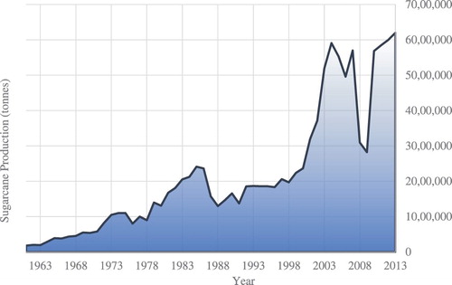
One of the main perennial crop is sugarcane, grown in tropical areas of various countries like India, Brazil, Thailand, China, Cuba, Pakistan, Mexico, and Iran. FAO, the food and agriculture organization of the United Nations stated that more than 90 countries are cultivating sugarcane within the area of 26.0 million hectares where the global harvest of sugarcane is 1.83 billion tons (FAO, 2015a). About 50% of the total sugar production in Iran is made from sugarcane, while about 90% of Iran’s sugarcane crop grows in Khuzestan province, located in the southern region of Iran. Attention to sugarcane plantation has been increased in recent years (Figure 1) not only for strained sugar source due to rapid population growth but also for a rising demand for the raw material of the sidelong industries such as ethanol, yeast, medium-density fibreboard (MDF) and single cell proteins. In view of the worldwide environment, sugarcane is a significant resource of alcohol to convert into biofuels for motor vehicles and electricity generation. Consequently, effective procedures for providing well-timed and precise information on sugarcane cultivation besides growth circumstances at regional and worldwide scales considered into attention.

Figure 1. Sugarcane production in Iran (FAO, 2015b).

Simplified models for the prediction of crop growth have become capable of effective implementation of estimation models for biophysical land use sustainability (Adam et al., 2010; Jeganathan, Roy, & Jha, 2010; Rugege, 2002; Willocquet et al., 2004). Such systems consider uptake water through roots, succeeding loss through transpiration and their impacts on crop growth. Many explanations, models and scheming of uptake water by roots depend on the plant condition, atmosphere and soil have been improved. The approaches vary extensively, established on the hydraulic laws of flow in porous mass media to attitudes that are basically instinctive extrapolations of experimental influence interactions, at the model level. Land use simulations require definite, numerical involvement data on, e.g. diurnal variant of atmospheric circumstances, impedance of plant organs, root density distribution, and movement of water through the soil. Accordingly, flow modelling from soil into the plant then to the atmosphere is too simple to be used in such a comprehensive land use investigation. The aforementioned data are not actually available regionally at farm. Therefore, simplified models are required to avoid such limitations.

Comparison of simple methods exposes an incompatible range of terminology and perceptions. Current study it an attempt to simulate the growth process of the sugarcane plantation using soft computing model on field data in south-west of Iran. As a result, the outputs of three different approaches were compared, statistically. Potential transpiration in plant has not been addressed in the current paper while the effects of cultivation parameters including daily grows (G), daily irrigation water (I), electric soil conductivity (EC), temperature (T), daily evaporation E (mm), wind speed (W), daily sunshine hours (S), and humidity (H) on sugarcane growth are considered. The methodologies deliberated were initially improved to apply in agronomic sugarcane systems.

Crop cultivation is difficult to model as it is a complex and nonlinear process. Soft-computing approaches have revealed efficient solutions for nonlinear natural process such as flood, drought, wind, and rainfall (Asadi, Shahrabi, Abbaszadeh, & Tabanmehr, 2013; Fortin, Anctil, Parent, & Bolinder, 2010; Gago, Martínez-Núñez, Landín, & Gallego, 2010; Lotfinejad et al., 2018; Moazenzadeh, Mohammadi, Shamshirband, & Chau, 2018; Mosavi, Bathla, & Varkonyi-Koczy, 2017; Nazari & Shamshirband, 2018; Sehgal, Sahay, & Chatterjee, 2014; Tiwari & Chatterjee, 2011). Some of the previous works have used soft-computing method for solving problem related to agriculture industry. (Kaul, Hill, & Walthall, 2005; Moayedi & Hayati, 2018) conducted a comprehensive review of research works that used various soft-computing procedures like artificial neural network (ANN), genetic algorithm (GP), and decision trees to study precision farming, crop growth, and food processing industry. Their work suggested concepts for using soft-computing approaches in agricultural and bio-engineering. Furthermore, (Osama, Mishra, & Somvanshi, 2015) used a feedforward multilayer ANN to relate sugarcane crop yield to climatic variable. Correspondingly, each model of the crop growth focused on one kind of product and one particular state of affairs. Several methods were established to model the similar procedure. For example, for modelling the biomass growth, a number of set of rules were applied. Several prototypes contained comprehensive explanation of the procedures associated with respiration and photosynthesis, even though other models procedure the radiation proficiency method as a representative of the comprehensive respiration and photosynthesis based on the one factor simulation.

At present, use of new computational method in answering the actual complications and formative the optimum values and tasks are getting high consideration by researchers of various scientific practices. One of these disciplines is ANN which has been utilized in many engineering applications. ANN is accomplished of solution for nonlinear complex problems that are problematic to answer classically by parametric approaches. Invisible Markov model (HMM) is an example of algorithms for preparation ANN. The weakness of ANN is the learning interval constraint. ELM is coined by Huang, Zhu, and Siew (2004) as a particular layer feedforward ANN. ELM algorithm is accomplished to resolve complications affected by gradient descent founded algorithms comparable back propagation that relates with ANN. Furthermore, ELM has the potential to empower the essential time for Neural Network training. Actually, it has been demonstrated that applying ELM, not only accelerates the learning process but also it produces forceful performance (Huang, Zhu, & Siew, 2006b). Consequently, a quantity of successful research works have been conducted utilizing ELM algorithm to solve the complications in several scientific areas (Ghouti, Sheltami, & Alutaibi, 2013; Nian et al., 2014; Wang & Han, 2014; Wang, Wang, & Yan, 2014; Wong, Wong, Vong, & Cheung, 2015; Yu, Miche, Séverin, & Lendasse, 2014).

ELM is generally an influential algorithm with more rapidly learning procedure, higher performance, smaller training error and weights norm in comparison with prior algorithms like back-propagation (BP) while ELM gets hold of better performance on consistency quantities (Zhong, Miao, Shen, & Feng, 2014). The remarkable acceleration established by ELM application is in line for antagonistic to communal ANN progress that depends on repetitive modification technique factors, the invisible layer biases and input weights of the model are indiscriminately allocated. However, considerably more rapidly than traditional ANNs, ELMs convince the universal rough calculation condition (Huang, Chen, & Siew, 2006), and make available superior generality presentations (Torabi, Hashemi, Saybani, Shamshirband, & Mosavi, 2018). In spite of these rewards, it was found that the potential of ELMs for data driven the growth of sugarcane forecasting applications has never been prospected. Therefore, filling this gap was the leading objective of our research work, where the appropriateness of ELM to establish rapid and truthful technique for crop production data-driven modelling is methodically evaluated. Nevertheless, previous research works have never investigated sugarcane growth using ELM. In current manuscript, the predictive model of sugarcane growing generated on the soft computing methodology, namely ELM is introduced. ELM was applied to establish a predictive model for forecasting the growth of sugarcane. The outcomes of the model were also compared with other NN methods like GP and also ANNs results to evaluate the accuracy of ELM model.

2. Description of the soft-computing model

2.1. Extreme learning machine

BP is a popular learning algorithm applied in feedforward neural networks (FFNN). In BP gradients are calculated competently by propagation commencing the output to the input (Sutskever, Vinyals, & Le, 2014). BP compacts with continuous data and recognizable stimulation tasks intended for single and multi-layer algorithms (Samet & Miri, 2012). BP procedure revealed certain regularly characteristic difficulties. As instant, BP procedure straightforwardly is confined in confined minima particularly for non-linearly distinguishable arrangement complications (Gori & Tesi, 1992; Zhang, Zhang, Lok, & Lyu, 2007), subsequently that BP possibly do not lead to find an over-all optimum answer. Moreover, the confluent speed of the BP is excessively slow in the learning objective, a given conclusion error, can be achieved. The main problematic is the dependence of the BP confluent behaviour algorithm on the selections of primary principles of the network link weights along with the factors in the procedure like the momentum and the learning rate (Ahmad, 1992; Van Ooyen & Nienhuis, 1992). ANN, as a most important computational method, was presented and used in various engineering arenas through the former decades. This technique solves nonlinear complications that are problematic for conventional mathematical methods. Several algorithms have been conducted for preparation ANN (Gholami, Chau, Fadaee, Torkaman, & Ghaffari, 2015; Olyaie, Banejad, Chau, & Melesse, 2015; Wang, Chau, Xu, Qiu, & Liu, 2017).

A miscellaneous predicting prototypical conjoining neural networks with fuzzy pattern-recognition was developed in view of the fuzziness in the perception of analogous basins, in which initiation tasks in the ANN model are improved with categorization (Ameli, Hemmati-Sarapardeh, Schaffie, Husein, & Shamshirband, 2018; Chau, 2017; Mosavi & Rabczuk, 2017b; Mosavi, Rabczuk, & Varkonyi-Koczy, 2017). Such a fuzzy pattern appreciation initiation task was presented addicted to a hybrid neural network (HNN) model to represent uncertainties of the river flow problematic (Chen, Chau, & Busari, 2015). Learning time requisite is the ANN deficiency. Consequently, Huang et al. (2004) proposed a single layer FFNN known as ELM algorithm, highly efficient in solving the complications initiated by gradient background. Furthermore, it decreases the essential time for ANN training. Moreover, for processing ELM algorithm no considerable human intervention is required, consequently, it can run considerably more rapidly than the ordinary procedures. It was demonstrated that by applying the ELM, the learning procedure develops fast with leading to a tough performance (Mosavi & Rabczuk, 2017a; Najafi, Faizollahzadeh Ardabili, Mosavi, Shamshirband, & Rabczuk, 2018). In view of that, several research works have been effectively conceded utilizing ELM algorithm for answering the complications in a number of scientific arenas. The significant of ELM algorithm has been proved with several advantages together with simple use, rapid learning speed, advanced performance, and appropriateness in various nonlinear initiation and kernel tasks (Ghouti et al., 2013; Nian et al., 2014; Taormina & Chau, 2015; Wang & Han, 2014; Wang et al., 2014; Wong et al., 2015; Yu et al., 2014).

2.2. Individual invisible layer for feedforward ANN

Single hidden layer feedforward neural network (SLFN) with L invisible nodes are categorized as an integrated and flexible mathematical model of radial basis function (RBF) network with invisible nodes of a_i and b_i as described by Huang et al. (2006) and Liang, Huang, Saratchandran, and Sundararajan (2006): (1) where according to Huang, Zhu, and Siew (2006a), the weight of β_i connects the ith node to the new node is provided by with initiation task of for preservative invisible node described as (2) x is the inner artefact of vector a_i and x in Rⁿ, and b_i is the bias of a_i. Where the weight vector a_i connects the input layer to the ith invisible node. Thus, a RBF network is special variation of SLFN with invisible layers. Furthermore, initializes the invisible nodes of RBF where, , described as: (3) where the core and effect factor of ith RBF node is characterized with a_i and b_i. The R⁺, further clarifies the positive and real values. is defined for N separate trials where input vector of t_i and x_i is m × 1 and n × 1, respectively. Thus, SLFN with L invisible nodes provides an accurate estimation of N trials and a_i, b_i and β_i are obtained as follows according to Huang et al. (2006a). (4) Equation (4) is written closely as (5) where (6) where (7) H is a matrix of representative invisible layer of outcome of SLFN where ith column of matrix representing the nodes of inputs of .

2.3. Foundation of ELM

Ghouti et al. (2013) describes ELM as a SLFN which has invisible neurons of for efficient learning of separate trials. The quantity of invisible neurons (L) depends on the quantity of separate trials (N). Through providing individual minor error ε > 0, the ELM can estimate the weights via pseudo opposite of H, leading to allocate accidental factors. However, adjusting the a_i and b_i during the training phase in ELM is highly simplified to well be allocated by means of accidental amounts. These actions are described in the subsequent statements.

Theorem 1:

According to Liang et al. (2006), a SLFN via L preservative and g(x) of the initiation task which is stated in interval of R. However, the earlier form of arbitrary L separate input vectors and could be produced by means of constant probability distribution, in turn. Besides, the matrix of the invisible layer output can be transformed through the probability one. Thus, the matrix H of the SLFN is considered invertible: .

Theorem 2:

According to Liang et al. (2006), it is assumed that the minor positive values (ε > 0) and for initialization, where and for N input vectors where produced distribution of continuous probability which the possibility is equal to one.

In the meantime, the invisible node factors of ELM do not require to be adjusted during the training phase due to the allocation of the random amounts. According to Equation (5), proposed by Huang et al. (2006a), the invisible node factors are transformed into a linear coordination and therefore, the final weights can be described: (8) Here is the inverse matrix of H representing the Moore–Penrose comprehensive invisible layer output. Singh and Balasundaram (2007) propose that can be computed using a wide choice of methods, e.g. orthogonal prediction or singular value decomposition (SVD). Here, the implementation of ELM is conducted through SVD to provide the Moore–Penrose generalized inverse of H. Thus, ELM presents a procedure for batch learning.

3. Experimental procedures

3.1. Description of the study site

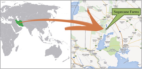
Sugarcane cultivation is the prevailing agriculture activities in the farm-lands of the southern Khuzestan province in Iran (Figure 2). The sugarcane farms consists of a 5 core zone (60,000 ha) (Hamdi, Baniabbasi, Almani, & Babagoli, 2005; Karimi, RajabiPour, Tabatabaeefar, & Borghei, 2008). The average air temperature is 24°C. Total annual rainfall is around 200 mm and sugarcane cultivation depends almost totally on the irrigation water from the rivers (Barzegar, Asoodar, & Ansari, 2000). As a common practice in the irrigation method for sugarcane production, the water is provided for farm irrigating by buried pipes, where water is distributed by furrow in the farm using flexible polyethylene gated pipe (Taherei Gazvinei, 2007).

Figure 2. Site of the sugarcane farm in Khuzestan state of Iran.

The functional unit is a sugarcane farm of 25 ha area where the slope direction is north-southward with the amount of 0.001 and 0.0003%. The total land area is 15,900 ha, where sugarcane is cultivated in the area of 12,000 (Dashtegol, Kashkooli, Naseri, & Nasab, 2009). Generally, based on the Unified Soil Classification System, soil texture is silt clay loam (Bahrani, Shomeili, Zande-Parsa, & Kamgar-Haghighi, 2010).

3.2. Field measurements

The input parameter and corresponding sources are presented in Table 1. Required data of the inputs quantities in sugarcane production were obtained principally from a daily activities, field measurement and secondary data.

Table 1. Input parameters used in the study.

Inputs parameters	Symbol (unit)	Maximum	Mean	Minimum	Standard deviation
Maximum daily temperature	Tmax (°C)	48.80	40.87	27.60	5.69
Daily evaporation	E (mm)	26.40	13.24	2.28	4.60
Mean daily wind speed	Wmean (m/s)	8.00	3.21	1.10	1.44
Total daily sunshine hours	ST (hour)	12.18	9.67	0.32	2.42
Daily rainfall	R (mm)	5.30	0.09	0.00	0.61
Mean daily humidity	Hmean (%)	69.00	47.69	28.00	8.11
Daily water irrigation	I (mm)	21.11	10.15	4.35	0.06
Measured electrical conductivity of soil	EC (ds/m)	2.20	1.40	0.86	0.27

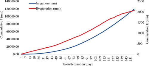
Irrigation and yield records of the sugarcane farm (Figure 3) were obtained from the records of the daily irrigation. Furthermore, data were scrutinized for errors and bias. The farm received 1575 mm of net irrigation, overall. Daily samples of the full-length stems were collected from different parts of the farm from the planting to the harvesting phase. Thus, mean daily growth of the sugarcane samples was calculated as daily growth of the farms sample. In addition to define EC (ds/m), soil of the farm was analysed daily in three depths from 0 to 90 cm with the interval of 30 cm.

Figure 3. Accumulative daily E and I in this study.

Daily field and climatological data of the sugarcane farm were collected. Field data including the amount of daily water irrigation (I), soil electric conductivity (EC), and growth of sugarcane (G). Besides, climatological information for growth simulation included daily maximum temperature (T_max), evaporation (E), sunshine hours (S), rainfall precipitation (R), humidity percentage (H), and mean wind speed (W) at 2 m above ground. Furthermore, weather information from the nearest active meteorological station was use.

Daily sugarcane growth (Table 2) was used in simulation by ELM in combination with ANN, and BP considering other input data. Finally, simulated results were compared with the observed daily sugarcane growth at the corresponding duration.

Table 2. Output parameters used in this study.

Output parameters	Symbol (unit)	Maximum	Mean	Minimum	Standard Deviation
Daily sugarcane growth	G (cm)	3.64	1.84	0.00	0.98

3.3. Input and output variables

Six input parameters selected for analysis in this study are shown in Table 1 including T_max (°C), evaporation (mm), wind speed (m/s), sunshine (hour), rainfall (mm), humidity (%), irrigation (mm), and EC (ds/m). These parameters are considered potentially influential for the sugarcane growth as the modelling output parameter (Table 2).

4. Results and discussion from measured data

The parameters of the crop were obtained as data by field trials of selected sugarcane variety. Data were measured carefully during field trials. Then, they were used to predict the daily sugarcane growth to compare with daily measured sugarcane growth.

Figure 3 shows accumulated daily evaporation within the accumulative daily irrigation water. Figure 3 indicates most of the portion of irrigation water was used to growth of the sugarcane and leaching to decrease the soil EC.

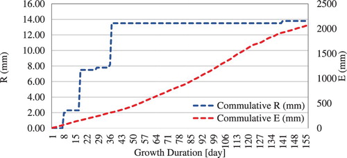
In addition, cumulative daily evaporation has been plotted against accumulative daily rainfall in Figure 4. It shows that after the 37th day of growing duration no significant rainfall was occurred. As the sugarcane farm is located at the semi-arid area, most of the required water consumption for growing stages of sugarcane was supplied by irrigation water.

Figure 4. Accumulative daily E and R in this study.

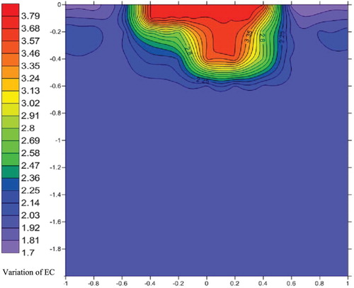
In the area of sugarcane root growth, the soil electrical conductivity (EC) was extracted from the soil layers indicated in Section 3.2. The average of measured EC were 3.3, 2.3, and 2.10 ds/m for the layers first to the third layer, respectively (Figure 5). EC indicators specify that after a number of irrigations the soils have altered salinity. Such a status maybe is due to the influence of several parameters. Consequently, measuring the electrical soil conductivity was extended to 2 m depth from the soil surface.

Figure 5. Change of EC (ds/m) in the soil of the sugarcane plant area.

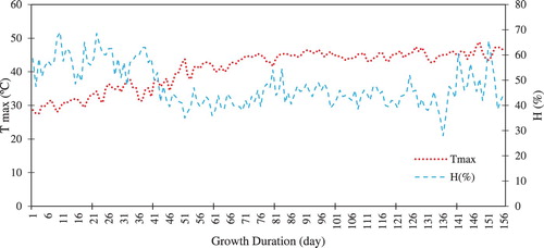
Maximum daily temperature is plotted against daily humidity in Figure 6. This figure shows that the maximum observed temperature was 48.8°C at the 148th day of the growth period. On the other hand, the maximum humidity of 69% was recorded on 10th day of the growth period. By and far, it was observed that increasing temperature resulted in the decrease of the humidity.

Figure 6. Observed daily maximum temperature (T_max) vs. H (%).

Observation showed that the final length of the sugarcane at the end of growth duration was 287 cm (Figure 7).

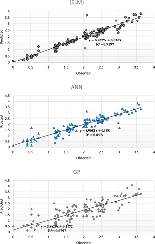
Figure 7. Predicted and observed values of the growth in training period of ELM, ANN, and GP models.

5. Results and discussion of soft-computing model

5.1. Models evaluation

Accuracy of projected methods were defined as coefficient of determination (R²), Nash–Sutcliffe efficiency (NS), and root means square error (RMSE), (Ayatollahi, Hemmati-Sarapardeh, Roham, & Hajirezaie, 2016; Hemmati-Sarapardeh & Mohagheghian, 2017). These statistics parameters are indicated as

1. R²: coefficient of determination (13)

2. RMSE: root-mean-square error, (14)

• (iii) Nash–Sutcliffe efficiency (NS) (15)

  where P_i and O_i present predicted and observed growth values of sugarcane, respectively, n is a representative of the number of test data.

5.2. Validation of the projected methods

In this section, the accuracy of the predictive models, predicting growth of the sugarcane, is reported. The specification of the ELM, ANN, and GP procedures are indicated in Tables 3–5, respectively. It is evident that ELM performs better predicted due to higher hidden layer compared with ANN. Such a better performance of ELM cannot be deducted from Table 5, while comparing the accuracy of predicted data generated by ELM and GP methods versus observed data, shows more accurate predicted sugarcane growth for ELM than GP (Figure 7).

Table 3. The ELM structure used in this study.

	Number of neurons
Number of layers	Input layer	Hidden layer	Output layer	Training rule	Activation function
3	8	35	1	ELM	Sigmoidal

Table 4. The ANN structure used in this study.

	Number of neurons
Number of layers	Input layer	Hidden layer	Output layer	Training rule	Number of iterations
3	8	25	1	Lavenberg–Marquardt	150

Table 5. The best parameters for the GP model used in this study.

Population size	Number of genes	Crossover probability	Mutation probability	Selection method
250	8	0.75	0.25	Tournament

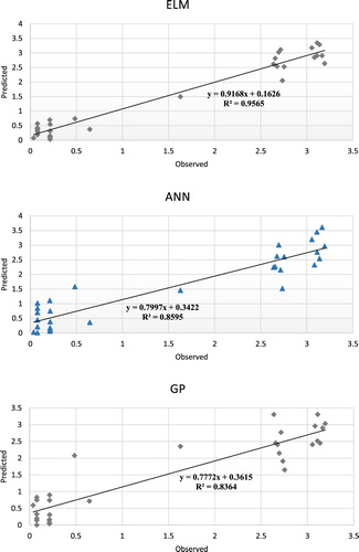
Figure 7 illustrates the rate of accuracy corresponding with established predictive models for the growth of sugarcane for all four stations in training period. Consequently, Figure 8 illustrates the accuracy of established ELM, ANN and GP of the growth models of the sugarcane, respectively in testing period. It is a proof that the more points in ELM graph are located alongside the line of perfect agreement. Moreover, predicted growths are in a reliable agreement with the recorded growths for ELM model. Therefore, it is confirmed that there is a high value for determination coefficient.

Figure 8. Predicted and observed values of the growth in testing period of ELM, ANN, and GP models.

5.3. Comparison of the models’ performance

In order to evaluate the projected models and to specify their performance, the models’ statistical parameters were compared. Statistical merits, r, RMSE and R² were applied in this comparison. Accuracy of the predicted results is indicated in Table 3.

Table 6 indicates that predicted daily sugarcane growths by ELM were more reliable than the ANN and GP as RMSE of the ELM is closer to 0.00 while corresponding R² of the ELM are the closer to 1.00 than the corresponding of ANN and GP in both training and testing periods. Therefore, predicted daily growth of sugarcane was plotted against the observed growth.

Table 6. Performance statistics comparison of the ELM, ANN and GP models.

	Training period			Testing period
Model	RMSE	R^2	NS	RMSE	R^2	NS
ELM	0.2423	0.9197	0.915	0.2887	0.9565	0.953
ANN	0.3184	0.8574	0.853	0.5138	0.8595	0.854
GP	0.5139	0.6797	0.619	0.5519	0.8364	0.831

6. Conclusion

The whole systems analysis is an essential technology that can cope with complexity and variability in delivering benefits to industry and in ensuring research efficiency in a complex operating environment. Central to this approach is the need to advance models for practical applications in industry. Strategic research is required to enhance the knowledge of simulation and optimization models. Delivery research is required to develop implementation strategies for the use of these tools in a participatory manner, to ensure adoption of new options for enhancing whole industry profitability in harmony with other sustainability considerations. The study of water, soil conductivity and sugarcane environment conditions presented in this paper have provided insights to the most effective and practical options for profitable and sustainable sugar production.

The research conceded a logical method to generate the ELM growth predictive model of the sugarcane. An evaluation of ELM method by way of ANN and GP techniques has been conducted to evaluate the model accuracy. According to the evaluation results, 0.95, 0.86, and 0.84 illustrated better performance in standings of R² in testing period, while RMSE of the statistical analysis of the ELM compare with the same statistics of ANN and GP. Statistical analyses of the ELM were more reliable than others. Besides, predicted daily growth of the sugarcane by ELM trend with the R² = 0.92 as similar as observed daily growth.

ELM model showed interesting and notable abilities which mark it distinct from former traditional gradient-based procedures of neural networks. Moreover, it was revealed that ELM is considerable quicker in learning rapidity in comparison with the conventional ANNs algorithm. Furthermore, the ELM model performed with the minimum norm of weights and the least training error while such an applicability did not appear in the traditional learning algorithms.

Selected soft computing methods were data-driven approaches that characterizes their main limits. These methods had a high dependency to the training data range while, in case of the existence some errors in the set of trained data, soft computing approaches can reduce the final error as they are extremely robust procedures on data variations. The most significant function through the training data preparation is to consider all probable conditions in the data to permit the soft computing systems to proceed the functions in all situations. Supplementary research works should validate whether the applied models could make available extra advantages when applied in by extraordinary nonlinearity of the crops production. Improved performances over other ELM method should also be probable to apply in various farms with insignificant interdependency between the variables.

Disclosure statement

No potential conflict of interest was reported by the authors.

ORCID

Pezhman Taherei Ghazvinei http://orcid.org/0000-0001-9186-7109

Shahaboddin Shamshirband http://orcid.org/0000-0002-6605-498X

References

- Adam, M., Ewert, F., Leffelaar, P. A., Corbeels, M., Van Keulen, H., & Wery, J. (2010). CROSPAL, software that uses agronomic expert knowledge to assist modules selection for crop growth simulation. Environmental Modelling & Software, 25(8), 946–955. %@ 1364–8152. doi: 10.1016/j.envsoft.2010.02.007
- Ahmad, M. (1992). Supervised learning using the Cauchy energy function. Proc. Int. Conf. on Fuzzy Logic and Neural Network.
- Ameli, F., Hemmati-Sarapardeh, A., Schaffie, M., Husein, M. M., & Shamshirband, S. (2018). Modeling interfacial tension in N2/n-alkane systems using corresponding state theory: Application to gas injection processes. Fuel, 222, 779–791. doi: 10.1016/j.fuel.2018.02.067
- Asadi, S., Shahrabi, J., Abbaszadeh, P., & Tabanmehr, S. (2013). A new hybrid artificial neural networks for rainfall–runoff process modeling. Neurocomputing, 121, 470–480. %@ 0925-2312. doi: 10.1016/j.neucom.2013.05.023
- Ayatollahi, S., Hemmati-Sarapardeh, A., Roham, M., & Hajirezaie, S. (2016). A rigorous approach for determining interfacial tension and minimum miscibility pressure in paraffin-CO2 systems: Application to gas injection processes. Journal of the Taiwan Institute of Chemical Engineers, 63, 107–115. doi: 10.1016/j.jtice.2016.02.013
- Bahrani, M., Shomeili, M., Zande-Parsa, S., & Kamgar-Haghighi, A. (2010). Sugarcane responses to irrigation and nitrogen in subtropical Iran. Iran Agricultural Research, 27–21. .2), pp. 17–26.
- Barzegar, A., Asoodar, M., & Ansari, M. (2000). Effectiveness of sugarcane residue incorporation at different water contents and the proctor compaction loads in reducing soil compactibility. Soil and Tillage Research, 57(3), 167–172. doi: 10.1016/S0167-1987(00)00158-6
- Chau, K.-W. (2017). Use of meta-heuristic techniques in rainfall-runoff modelling. Multidisciplinary Digital Publishing Institute.
- Chen, X., Chau, K., & Busari, A. (2015). A comparative study of population-based optimization algorithms for downstream river flow forecasting by a hybrid neural network model. Engineering Applications of Artificial Intelligence, 46, 258–268. doi: 10.1016/j.engappai.2015.09.010
- Dashtegol, A., Kashkooli, H., Naseri, A., & Nasab, S. (2009). Effects of every-other furrow irrigation on water use efficiency and sugarcane characteristics in southern Ahvaz sugarcane fields. Journal of Science and Technology of Agriculture and Natural Resources, 13(49 (B)), 45–58.
- FAO. (2015a). Crop production. F. a. A. O. o. t. U. Nations.
- FAO. (2015b). Sugarcane production. Author.
- Fortin, J. G., Anctil, F., Parent, L-É, & Bolinder, M. A. (2010). A neural network experiment on the site-specific simulation of potato tuber growth in Eastern Canada. Computers and Electronics in Agriculture, 73(2), 126–132. %@ 0168-1699. doi: 10.1016/j.compag.2010.05.011
- Gago, J., Martínez-Núñez, L., Landín, M., & Gallego, P. P. (2010). Artificial neural networks as an alternative to the traditional statistical methodology in plant research. Journal of Plant Physiology, 167(1), 23–27. %@ 0176-1617. doi: 10.1016/j.jplph.2009.07.007
- Gholami, V., Chau, K., Fadaee, F., Torkaman, J., & Ghaffari, A. (2015). Modeling of groundwater level fluctuations using dendrochronology in alluvial aquifers. Journal of Hydrology, 529, 1060–1069. doi: 10.1016/j.jhydrol.2015.09.028
- Ghouti, L., Sheltami, T. R., & Alutaibi, K. S. (2013). Mobility prediction in mobile ad hoc networks using extreme learning machines. Procedia Computer Science, 19, 305–312. doi: 10.1016/j.procs.2013.06.043
- Gori, M., & Tesi, A. (1992). On the problem of local minima in backpropagation. IEEE Transactions on Pattern Analysis and Machine Intelligence, 14(1), 76–86. doi: 10.1109/34.107014
- Hamdi, H., Baniabbasi, N., Almani, M. P., & Babagoli, S. (2005). Advances in TAE Sugarcane Breeding Program in Iran. Proc. ISSCT.
- Hemmati-Sarapardeh, A., & Mohagheghian, E. (2017). Modeling interfacial tension and minimum miscibility pressure in paraffin-nitrogen systems: Application to gas injection processes. Fuel, 205, 80–89. doi: 10.1016/j.fuel.2017.05.035
- Huang, G.-B., Chen, L., & Siew, C. K. (2006). Universal approximation using incremental constructive feedforward networks with random hidden nodes. IEEE Transactions on Neural Networks, 17(4), 879–892. doi: 10.1109/TNN.2006.875977
- Huang, G.-B., Zhu, Q.-Y., & Siew, C.-K. (2004). Extreme learning machine: a new learning scheme of feedforward neural networks. Neural Networks, 2004. Proceedings. 2004 IEEE International Joint Conference on.
- Huang, G.-B., Zhu, Q.-Y., & Siew, C.-K. (2006a). Extreme learning machine: Theory and applications. Neurocomputing, 70(1), 489–501. doi: 10.1016/j.neucom.2005.12.126
- Huang, G.-B., Zhu, Q.-Y., & Siew, C. K. (2006b). Real-time learning capability of neural networks. IEEE Transactions on Neural Networks, 17(4), 863–878. doi: 10.1109/TNN.2006.875974
- Jeganathan, C., Roy, P. S., & Jha, M. N. (2010). Markov model for predicting the land cover changes in Shimla district. Indian Forester, 136(5), 667–686. 0019-4816.
- Karimi, M., RajabiPour, A., Tabatabaeefar, A., & Borghei, A. (2008). Energy analysis of sugarcane production in plant farms a case study in Debel Khazai agro-industry in Iran. American-Eurasian Journal of Agricultural and Environmental Science, 4, 165–171.
- Kaul, M., Hill, R. L., & Walthall, C. (2005). Artificial neural networks for corn and soybean yield prediction. Agricultural Systems, 85(1), 1–18. %@ 0308-0521X. doi: 10.1016/j.agsy.2004.07.009
- Liang, N.-Y., Huang, G.-B., Saratchandran, P., & Sundararajan, N. (2006). A fast and accurate online sequential learning algorithm for feedforward networks. IEEE Transactions on Neural Networks, 17(6), 1411–1423. doi: 10.1109/TNN.2006.880583
- Lotfinejad, M. M., Hafezi, R., Khanali, M., Hosseini, S. S., Mehrpooya, M., & Shamshirband, S. (2018). A comparative assessment of predicting daily solar radiation using bat neural network (BNN), generalized regression neural network (GRNN), and neuro-fuzzy (NF) system: A case study. Energies, 11(5), 1188. doi: 10.3390/en11051188
- Moayedi, H., & Hayati, S. (2018). Artificial intelligence design charts for predicting friction capacity of driven pile in clay. Neural Computing and Applications, 29(1), 1–17. doi: 10.1007/s00521-017-3243-x
- Moazenzadeh, R., Mohammadi, B., Shamshirband, S., & Chau, K.-w. (2018). Coupling a firefly algorithm with support vector regression to predict evaporation in northern Iran. Engineering Applications of Computational Fluid Mechanics , 12(1), 584–597. doi: 10.1080/19942060.2018.1482476
- Mosavi, A., Bathla, Y., & Varkonyi-Koczy, A. (2017). Predicting the future using web knowledge: State of the art survey. International Conference on Global Research and Education.
- Mosavi, A., & Rabczuk, T. (2017a). Learning and intelligent optimization for computational materials design innovation.
- Mosavi, A., & Rabczuk, T. (2017b). Learning and intelligent optimization for material design innovation. Learning and Intelligent Optimization: Springer.
- Mosavi, A., Rabczuk, T., & Varkonyi-Koczy, A. R. (2017). Reviewing the novel machine learning tools for materials design. Recent Advances in Technology Research and Education: Springer Nature.
- Najafi, B., Faizollahzadeh Ardabili, S., Mosavi, A., Shamshirband, S., & Rabczuk, T. (2018). An intelligent artificial neural network-response surface methodology method for accessing the optimum biodiesel and diesel fuel blending conditions in a diesel engine from the viewpoint of exergy and energy analysis. Energies, 11(4), 860. doi:10.3390/en11040860
- Nazari, M., & Shamshirband, S. (2018). The particle filter-based back propagation neural network for evapotranspiration estimation. ISH Journal of Hydraulic Engineering. doi: 10.1080/09715010.2018.1481462
- Nian, R., He, B., Zheng, B., Van Heeswijk, M., Yu, Q., Miche, Y., & Lendasse, A. (2014). Extreme learning machine towards dynamic model hypothesis in fish ethology research. Neurocomputing, 128, 273–284. doi: 10.1016/j.neucom.2013.03.054
- Olyaie, E., Banejad, H., Chau, K.-W., & Melesse, A. M. (2015). A comparison of various artificial intelligence approaches performance for estimating suspended sediment load of river systems: A case study in United States. Environmental Monitoring and Assessment, 187(4), 189. doi: 10.1007/s10661-015-4381-1
- Osama, K., Mishra, B. N., & Somvanshi, P. (2015). Machine Learning Techniques in Plant Biology. PlantOmics: The Omics of Plant Science (pp. 731-754%@ 8132221710): Springer.
- Rugege, D. (2002). Regional analysis of maize-based land use systems for early warning applications.
- Samet, S., & Miri, A. (2012). Privacy-preserving back-propagation and extreme learning machine algorithms. Data & Knowledge Engineering, 79, 40–61. doi: 10.1016/j.datak.2012.06.001
- Sehgal, V., Sahay, R. R., & Chatterjee, C. (2014). Effect of utilization of discrete wavelet components on flood forecasting performance of wavelet based ANFIS models. Water Resources Management, 28(6), 1733–1749. %@ 0920-4741. doi: 10.1007/s11269-014-0584-4
- Singh, R., & Balasundaram, S. (2007). Application of extreme learning machine method for time series analysis. International Journal of Intelligent Technology, 2(4), 256–262.
- Sutskever, I., Vinyals, O., & Le, Q. V. (2014). Sequence to sequence learning with neural networks. Advances in neural information processing systems.
- Taherei Gazvinei, P. (2007). Assessment the Changes of the Irrigation & Drainage Water Levels on the Sugarcane Growth and Production (PhD. Research and Science Azad University, Ahwaz.
- Taormina, R., & Chau, K.-W. (2015). Data-driven input variable selection for rainfall–runoff modeling using binary-coded particle swarm optimization and extreme learning machines. Journal of Hydrology, 529, 1617–1632. doi: 10.1016/j.jhydrol.2015.08.022
- Tiwari, M., & Chatterjee, C. (2011). A new wavelet-bootstrap-ANN hybrid model for daily discharge forecasting. Journal of Hydroinformatics, 13(3), 500–519. doi: 10.2166/hydro.2010.142
- Torabi, M., Hashemi, S., Saybani, M. R., Shamshirband, S., & Mosavi, A. (2018). A hybrid clustering and classification technique for forecasting short-term energy consumption. Environmental Progress & Sustainable Energy. doi: 10.1002/ep.12934
- Van Ooyen, A., & Nienhuis, B. (1992). Improving the convergence of the back-propagation algorithm. Neural Networks, 5(3), 465–471. doi: 10.1016/0893-6080(92)90008-7
- Wang, W.-c., Chau, K.-w., Xu, D.-m., Qiu, L., & Liu, C.-c. (2017). The annual maximum flood peak discharge forecasting using Hermite projection pursuit regression with SSO and LS method. Water Resources Management, 31(1), 461–477. doi: 10.1007/s11269-016-1538-9
- Wang, X., & Han, M. (2014). Online sequential extreme learning machine with kernels for nonstationary time series prediction. Neurocomputing, 145, 90–97. doi: 10.1016/j.neucom.2014.05.068
- Wang, D. D., Wang, R., & Yan, H. (2014). Fast prediction of protein–protein interaction sites based on extreme learning machines. Neurocomputing, 128, 258–266. doi: 10.1016/j.neucom.2012.12.062
- Willocquet, L., Elazegui, F. A., Castilla, N., Fernandez, L., Fischer, K. S., Peng, S., … Zhu, D. (2004). Research priorities for rice pest management in tropical Asia: A simulation analysis of yield losses and management efficiencies. Phytopathology, 94(7), 672–682. %@ 0031-0949X. doi: 10.1094/PHYTO.2004.94.7.672
- Wong, P. K., Wong, K. I., Vong, C. M., & Cheung, C. S. (2015). Modeling and optimization of biodiesel engine performance using kernel-based extreme learning machine and cuckoo search. Renewable Energy, 74, 640–647. doi: 10.1016/j.renene.2014.08.075
- Yu, Q., Miche, Y., Séverin, E., & Lendasse, A. (2014). Bankruptcy prediction using extreme learning machine and financial expertise. Neurocomputing, 128, 296–302. doi: 10.1016/j.neucom.2013.01.063
- Zhang, J.-R., Zhang, J., Lok, T.-M., & Lyu, M. R. (2007). A hybrid particle swarm optimization–back-propagation algorithm for feedforward neural network training. Applied Mathematics and Computation, 185(2), 1026–1037. doi: 10.1016/j.amc.2006.07.025
- Zhong, H., Miao, C., Shen, Z., & Feng, Y. (2014). Comparing the learning effectiveness of BP, ELM, I-ELM, and SVM for corporate credit ratings. Neurocomputing, 128, 285–295. doi: 10.1016/j.neucom.2013.02.054