Experiments and CFD modeling of high-velocity two-phase flows in a large chute aerator facility

ABSTRACT

Mathematical formulations of two-phase flows at an aerator remain a challenging issue for spillway design. Due to their complexities in terms of water–air interactions subjected to high flow velocities, experiments play an essential role in evaluations of numerical models. The paper focuses on the underlying influence of the air–water momentum exchange in the two-phase Two-Fluid Model. It is modified to better represent the drag force acting on a group of air bubbles and the wall lubrication force accounting for near-wall phase interactions. Based on data from a large aerator rig with an approach velocity of 14.3 m/s, the models are evaluated for calculations of entrained air characteristics of a flow mixture. The air bubble diameter used in the modeling ranges from 0.5 to 4 mm as suggested by the experiments. In terms of air cavity configurations and aerator air demand, smaller air bubbles lead to better agreement with the test results. As far as air concentrations are concerned, the modified model gains by comparison. In the air cavity zone, smaller bubble sizes also provide better matches with the experiments. However, the near-base air concentration remains overestimated downstream from the impact area. The fact that the program user must pre-define a single air bubble size in simulations presumably limits the correct reproduction of near-base air concentrations and of their decay.

KEYWORDS:

• Aerator
• two-phase flow
• two-fluid model
• drag force
• wall lubrication force
• air cavity

1. Introduction

Various types of two-phase mixtures are frequently encountered in facilities of chemical processes, and in related industries. Mixtures of water and other liquids (e.g. oil), of water and solid particles (e.g. sediment) or of water and gas (e.g. air and vapor) are found in Joshi (2001), Chau and Jiang (2001), Sokolichin, Eigenberger, and Lapin (2004), Chau and Jiang (2004), Ekambara, Dhotre, and Joshi (2005) and Wu and Chau (2006). Two-phase components are often immiscible. Depending on phase and flow conditions, flow regimes are categorized as either separated or dispersed flows. The former features a mixture of two phases of different densities with a sharp resolvable interface between them; the latter appears as two distinct phases with one phase dispersed in the other continuous medium (Drew & Lahey, 1993; Kolev, 1977).

The accurate prediction of a two-phase flow that is either steady or transient is of economic interest and is desirable in regard to safety concerns. Over the past few decades, several typical two-phase models have been developed and improved upon (ANSYS, 2015; Hibiki & Ishii, 2000; Hirt & Nichols, 1981; Kolev, 2005; Özkan, Wenka, Hansjosten, Pfeifer, & Kraushaar-Czarnetzki, 2016). These include the Volume-of-Fluid (VOF) Model, the Mixture Model and the Two-Fluid Model. Two-phase flow formulation, constitutive relations and empirical corrections form the basis of these models. Associated modeling difficulties are related to the formulation of interface transfers between two phases and discontinuities associated with them. Constitutive equations for interface interactions are the weakest link but are critical in the determination of phase dependence. Based on experiments and observations, interface terms are often corrected for different applications as shown in Ishii and Mishima (1984), Crawford, Weinberger, and Weisman (1985, 1986), Owen and Hewitt (1987), Michaelides (2003) and Tabib, Roy, and Joshi (2008).

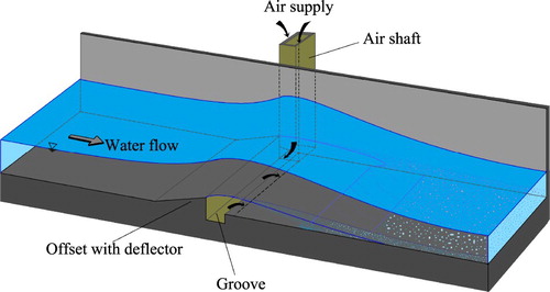
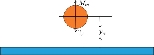
A spillway aerator is an installation constructed to artificially entrain air and to prevent the cavitation of concrete surfaces subjected to high-velocity flows (Bai, Zhang, Liu, & Wang, 2016; Falvey, 1980, 1990; Pfister & Hager, 2010a, 2010b; Volkart & Rutschmann, 1984; Wood, 1991). Cavitation damage must be inhibited as it progressively damages the spillway structure. Different aerator configurations with, e.g. offsets, deflectors (ramps), grooves and combinations of these features, have been developed. Figure 1 shows the sketch of water–air flow phenomenon occurring at the aerator. Downstream from an aerator, the deflected flow jet encloses an air cavity. Due to high velocities involved, air is entrained into the lower edge of the jet. The air-pressure gradient between the cavity and atmosphere generates airflows across the air supply system; the air flow rate is mainly dependent on the pressure difference and on the geometry of the air passage. Downstream from the cavity, the free flow jet is confined by the concrete surface and strong turbulent mixing occurs in the impact zone. The entrained air then becomes successively detrained. It is the entrained air in the immediate vicinity of the chute surface that prevents cavitation from occurring. Each aerator thus protects a limited chute area downstream (Chanson, 1994; ICOLD, 1987, 1992; Kramer, 2004; Kramer & Hager, 2005; Pinto, Neidert, & Ota, 1982).

Figure 1. Sketch of water-air flow phenomenon occurring at a spillway aerator.

In many industrial applications, flow velocities often amount to only a few meters per second. Aerator flows are operated at a much higher velocity, posing a challenge for numerical predictions. Depending upon the water head, the flow velocity can increase to as high as 30–45 m/s. From this high velocity, the exchange between the air and water becomes more intensive. This implies that formulations of phase interactions become more complex in an aerator flow. The main reason is lack of prototype measurement data for numerical model calibration and verification.

The VOF Model is sometimes used to simulate aerator flows (Deng, Xu, Lei, & Diao, 2005; Jothiprakash, Bhosekar, & Deolalikar, 2015; Kökpınar & Göğüş, 2002; Liu & Yang, 2014; Rahimzadeh, Maghsoodi, Sarkardeh, & Tavakkol, 2012). Aydin and Ozturk (2009) and Zhang, Chen, and Xu (2011) employ the Mixture Model to study an aerator flow and found that the model is more suitable for simulating aerator flows and especially in high air-concentration regions. Such studies focus on both experimental and prototype data and show that the model produces reasonable base pressure and air cavity profiles. Criticism of the two-phase model has however been raised by Chanson and Lubin (2010), who discuss Aydin and Ozturk’s approach to verifying aerator flows. They question the procedure of model verification and validation by means of a single parameter, i.e. the air-flow rate supplied by the air duct. Instead, it should be based upon detailed air–water flow properties at the spillway aerator and independent datasets.

The Two-Fluid Model can also be used to model aerator flows. Unlike the VOF model, it is based on interactions between air bubbles and water and involves the modeling of the phase drag force, turbulent dispersion force, etc. In related studies, numerical results are compared with experimental data (Xu, Wang, Tan, & Yang, 2001; Zhang, Liu, Zhan, & Wu, 2008). Though limited in number, such studies reveal the potential of modeling aerator flows. This motivates further examinations and evaluations of the Two-Fluid Model.

Numerically predicting the functions of aerators remains an issue of major concern in the realm of spillway design. Due to the complexities of water–air interactions, the mathematical formulation of the Two-Fluid Model involves the use of several coefficients and parameters that are either theoretical or empirical, the values of which should be evaluated against measured data from either prototypes or scale models. High-flow velocities, strong flow turbulence levels and mixing also necessitate model evaluations.

In the Two-Fluid Model, the drag force on air bubbles is considered; it is however derived from motions of single isolated bubbles (ANSYS, 2015; Schiller & Naumann, 1935). Furthermore, in the cavity, the water jet’s lower edge is a free surface with air entrainment; after the impact, the flow is confined by the chute base and air supplies cease. Corresponding spatial changes affect air bubble movement. The near-wall interaction effect, which is referred to as the wall lubrication force, is not considered in the model. Based on previous modeling experiences, the drag coefficient is modified to better represent the drag force acting on air bubbles. The drag force is now based on movements of a collection of bubbles, which is more reflective of reality. The wall lubrication force is also included and provides better approximations of bubble movements through the jet impact area.

Imposed by practical constraints, prototype observations and measurements are difficult to make; available data are fragmented and incomplete. Model tests are often used to obtain data necessary for numerical evaluations. However, limited by test facilities, flow velocities are usually below 7–8 m/s; higher model velocities would certainly allow for more meaningful comparisons. Aerator experiments were conducted in a large test rig with its upper chute end approximately 13 m above the floor, thus producing a flow velocity amounting to 15.4 m/s at the aerator. Based on the unique data obtained, the study addresses mainly the influence of the air–water momentum exchange term of the Two-Fluid Model. Its purpose is to evaluate its reliability and to provide guidance on the selection of two-phase models for engineering applications.

2. Experimental layout

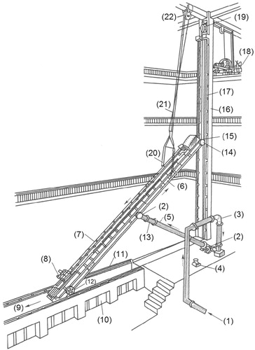
The aerator experiments were performed in a large test rig based at the Institute of Water Resources and Hydropower Research (IWHR) in Beijing (Shi, 2007; Zhang et al., 2008). With the construction of many large dams around the world, it was specifically designed for tests of chute aerators subjected to high flow velocities. The rig layout is shown in Figure 2. The main technical parameters of the facility are described below.

Figure 2. Spillway aerator test rig: (1) water from pump; (2) rotatable pipe joint; (3) flow meter; (4) regulating valve; (5) water-supply pipe; (6) water supply in flume bottom; (7) test flume with aerator; (8) 3D measurement carriage; (9) tail water; (10) observation window; (11) horizontal rail; (12) horizontally moving wheel on flume; (13) expansion pipe section; (14) vertically moving wheel; (15) water intake to flume; (16) counter weight (not shown); (17) vertical rail; (18) hoister; (19) safety brake; (20) lifting cradle; (21) lifting steel wire and guide wheel.

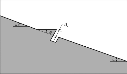
The aerator chute was l = 15 m long and b = 20 cm wide; both sides were surrounded by Plexiglas walls. The chute width was originally 50 cm. To obtain a larger water depth at a given flow rate, its width was reduced to 20 cm and a series of aerator tests was made. The slope of the chute was designed to be variable. Both ends of the flume were equipped with wheels that moved along their respective horizontal and vertical rails. Driven by a servomotor, it could be locked at any desired position. Its horizontal slope angle was adjusted to a range of α = 0–49° (Figure 3). At its maximum angle 49°, the upper chute end was positioned approximately 13 m above the laboratory floor. In the chute base, an air duct (groove) was built to cover the chute width without any offset but with replaceable deflectors of varying sizes. A pipe of sufficiently large diameter was connected to the duct on each side, through which air was sucked into the cavity. The height of the deflectors varied between Δ = 3–25 mm with a constant deflector angle of tanθ = 1:10.

Figure 3. Definition of aerator geometrical parameters.

Water was supplied by pumping it from an underground reservoir. As is shown in Figure 2, the feeding pipe (30 cm in diameter) was connected to a conduit running beneath and parallel to the flume, delivering water to the chute inlet. The expansion pipe section with a rotatable junction adapted itself to the desired flume slope angle. The chute inlet was formed as a rectangular conduit; it was 1.2 m long and was of the same width as the chute. At a given water flow rate, its height was typically adjusted to approximate the chute water depth. The purpose of the inlet layout was to dampen the turbulence and to supply uniform inflows of pure water into the flume. The outflow from the chute discharged into a tail-water flume and returned to the underground reservoir.

In the test rig, monitored flow parameters included the water-flow rate (Q_w), streamwise water-flow velocity, water depth, entrained air flow rate (Q_a), chute-base pressure level, air cavity under-pressure level, air-cavity shape including the jet trajectory length and air concentration (C). Equipped with a 3D positioning system, an instrument carrier operated along the rails of the flume to collect water velocity, water depth and C measurements. The measurement of a parameter at a given position was as a rule repeated 4–6 times; its value referred to its time-averaged value.

Measurements of Q_w were made using two devices – a flow meter and an overflow weir. Both were calibrated. Their relative errors of measurement were less than ±3% and ±1%, respectively. Air was supplied to the cavity through a lateral duct. Based on the air inlet area, the Q_a value was determined by a calibrated airflow anemometer with an inaccuracy level of less than ±(1.5−2)%. In the jet impingement area, several pressure transducers were mounted at the chute base to detect the maximum chute pressure position in the flow direction. The air pressure in the cavity was also monitored with air pressure transducers.

A propeller-type water-flow velocimeter was used to measure the flow velocity in the flume with an inaccuracy level of below ±(2−4)%. Water depths were directly measured with a point gauge and referred to the depth in the direction perpendicular to the flume. For a given cross-section, the obtained water depth result was also checked against Q_w and its flow velocity. Measurements of flow velocity and water depth were made in the so-called black-water area upstream from the air cavity. By black water we mean, as in other studies of water–air flows, pure-water body that is not affected or penetrated by entrained air.

Measurements of the spatial C distribution were realized by two means: a direct sampling device and a resistance-type probe. The former featured a closed system for air–water sampling, separation and measurement, allowing for a long sampling period to guarantee the acquisition of the time-averaged C value at a given location. As the tip inner diameter of its probe must be larger than the size of air bubbles, diameters of 3 to 7 mm were available for use. However, as the device was inconvenient to operate, it was mainly used for calibration purposes (Shi, 2007).

A resistance-type probe featuring a probe with two tips positioned 6 mm apart was a frequently used. Each tip was composed of two thin plates of stainless steel of 1 mm thick, 6 mm wide and 25 mm long. Its measurement principle was based on the difference in conductivity levels between water and air. When the air concentration changed at the probe, the resistance between its two tips would change accordingly. Similar probes have been used by Chanson (1997), Matos and Frizell (1997), Chanson and Toombes (2002), Pfister and Hager (2010a, 2010b) and Bai et al. (2016). The sampling frequency of the probe ranged from 2000–3000 Hz. Necessary structural reinforcements were needed to withstand high-velocity flows. For quality control purposes, benchmark tests were carried out using eight (8) probes of different manufacturers. We found that the discrepancy in C values between them was less than ±(3–4)%. Calibrations were made to reduce measurement errors; the C uncertainty value was usually less than ±2%.

The Q_w value of the rig was adjustable with the help of the regulating valve with its maximum value being 0.342 m³/s. The maximum Q_a value in the aerator amounted to 0.0756 m³/s. The approaching flow velocity and water depth at the aerators amounted to u₁ = 6.6–15.4 m/s and h₁ = 0.050–0.251 m, respectively. Both u₁ and h₁ were measured at the ends of the deflectors. The aerator Froude number, F = u₁/(gh₁)², ranged from 4.34 to 21.90 where g = gravitational acceleration (m/s²); Reynolds numbers, R = ρ_wu₁h₁/μ_w, varied from (0.69–1.41) × 10⁶ where μ_w = the viscosity of water (Pa·s) and ρ_w = the density of water (kg/m³).

During the experiments, measurements of C were made at 13 cross-sections. These are denoted as S1–S13 and are positioned perpendicular to the chute base (Table 1). The distance between two neighboring locations is not equal. S1–S11 are upstream from point S and S12–S13 are positioned downstream.

Table 1. Cross-sectional positions.

	S1	S2	S3	S4	S5	S6	S7	S8	S9	S10	S11	S12	S13
x (m)	0.4	0.6	0.8	1.0	1.2	1.5	1.8	2.0	2.2	2.4	2.6	3.0	3.5

Experimental results for C are given in Table 2. Each value is the result of the spatial averaging of a few transverse points in the center of the chute.

Table 2. Experimental results of C at S1–S13.

	C (%)
z (cm)	S1	S2	S3	S4	S5	S6	S7	S8	S9	S10	S11	S12	S13
0.80	84	96	97	97	96	92	81	70	61	55	51	46
1.30	80	94	95	96	95	93	85	77	66	56	51	47
1.75	76	91	94	94	94	91	82	77	67	57	52	48	44
2.65	51	84	87	88	87	83	77	71	65	59	52	48	47
3.85	14	69	74	77	76	71	66	65	61	63	59	53
5.00	3	55	58	61	61	58	54	58	62	67	67	62	57
6.25	3	29	39	47	48	50	58	61	63	68	73	70	74
7.40	9	24	36	43	40	48	59	63	71	73	72	82	81
8.70	49	17	25	37	45	55	67	74	74	74	85	86	89
10.0	89	53	43	44	52	60	70	75	79	82	89	89	91
11.2	95	75	74	71	67	72	75	79	81	87	83	86	92
12.2	97	89	83	76	75	75	79	86	82	90		91	94
13.4	97	96	93	88	84	85	86	89	87	91	91	92
14.6			94	92	90	89	89	88	91	91		92
17.2			97	96	95	93	93	93	94	94	94	95
20.7					96	96	96	96	95	95	95	96

A limited number of measurements were made to estimate equivalent diameters of air bubbles of the entrained air from the cavity. No tests were conducted on the upper jet free surface. The results indicate that downstream from the cavity, sizes increase somewhat with water depth and in the flow direction. Within two cavity lengths from the aerator, the averaged diameter that accounts for approximately 85% of the data is above 0.5 mm and below 4 mm. The Two-Fluid Model allows for input of only one air bubble D specified explicitly by the modeler. Within this range, four D values are used in numerical modeling to examine the effect of bubble sizes on the predictions, i.e. D = 0.5, 1, 2, 4 mm.

One must be aware that air bubble sizes are strongly dependent on Reynolds numbers, which vary from one location to another in aerator flow fields and which are thus subject to scale effects in a Froude model (Chanson & Toombes, 2002).

3. Numerical model

3.1. Aerator setup

The configuration of aerator flows used is illustrated in Figure 4, in which a 2D coordinate system (x, z) is defined. The x-coordinate is located on the chute base (positive downwards); the z-coordinate is positioned perpendicular to the chute base and coincides with the downstream face of the deflector (positive upwards). Table 3 shows the representative test conditions adopted as a basis for the numerical simulations. Parameters q_w and q_a refer to unit water and air flow rates (q_w = Q_w/b, q_a = Q_a/b).

Figure 4. Aerator flow configuration: (1) approach flow; (2) transition; (3) cavity nappe; (4) impact; (5) downstream flow.

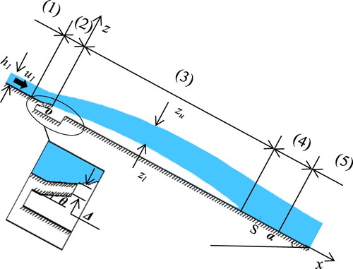
Table 3. Aerator geometry and flow conditions in CFD modeling.

	Δ	Qw	qw	h1	u1	Qa	qa		Re
α (°)	(mm)	(m^3/s)	(m^2/s)	(cm)	(m/s)	(m^3/s)	(m^2/s)	Fr	(10^6)
49	15	0.342	0.827	5.8	14.27	0.0756	0.375	18.9	0.69

3.2. Two-fluid model

An aerator flow is a typical two-phase flow. The Two-Fluid Model, an Euler-Euler model, is a two-phase two-fluid model used to reproduce the flow field. The Fluent software in ANSYS (2015) is used for the simulations.

The framework of the Two-Fluid Model is based on ensemble-averaged mass and momentum transport equations for each of the two phases. Continuity and momentum equations of each phase are given as

Continuity equation (1) $\frac{\mathrm{\partial }}{\mathrm{\partial }t}\left({\alpha }_i{\rho }_i\right)+\mathrm{\nabla }\cdot \left({\alpha }_i{\rho }_i{\stackrel{\rightharpoonup }{v}}_i\right)=0$(1) where α = the phase volume fraction, ρ = the phase density, $\stackrel{\rightharpoonup }{v}$ = the phase velocity and t = the time. Here, subscript i denotes the air phase (a) and water phase (w).

Momentum equation (2) $\begin{array}{rl}& \frac{\mathrm{\partial }}{\mathrm{\partial }t}\left({\alpha }_i{\rho }_i{\stackrel{\rightharpoonup }{v}}_i\right)+\mathrm{\nabla }\cdot \left({\alpha }_i{\rho }_i{\stackrel{\rightharpoonup }{v}}_i{\stackrel{\rightharpoonup }{v}}_i\right)=-{\alpha }_i\mathrm{\nabla }p\\ & +\mathrm{\nabla }\cdot {\overline{\tau }}_i+{\alpha }_i{\rho }_{i}g+G+M\end{array}$(2) where $\mathrm{\nabla }p$ = the pressure gradient, G = the interphase force between water and air (per unit volume of mixture), M = the interfacial force (per unit volume of mixture) and τ = the stress–strain tensor expressed as follows. (3) ${\overline{\tau }}_i={\alpha }_i{\mu }_i(\mathrm{\nabla }{\stackrel{\rightharpoonup }{v}}_i+\mathrm{\nabla }{\stackrel{\rightharpoonup }{v}}_i^T)+{\alpha }_i({\zeta }_i-\frac{2}{3}{\mu }_i)\mathrm{\nabla }{\stackrel{\rightharpoonup }{v}}_i\overline{I}$(3) where ζ = the phase bulk viscosity and I = the identity tensor.

The interphase force G consists of water–air friction, pressure, cohesion and other effects and is written as follows (4) $G_{aw}=-G_{wa}=K_{aw}({\stackrel{\rightharpoonup }{v}}_a-{\stackrel{\rightharpoonup }{v}}_w)$(4) where K_aw = the interphase exchange coefficient between water and air phases and it is dependent on the drag function f (dimensionless number). (5) $K_{aw}=\frac{{\rho }_{a}f}{6{\tau }_a}DA$(5) where A = the interfacial area between water and air and τ_a = the particulate relaxation time.

Air bubbles are assumed to be spherical. The interfacial force M refers to the interfacial momentum exchange composed of four terms, namely, the lift force M_l, the turbulence dispersion force M_td, the virtual mass force M_vm and the wall-lubrication force M_wl. The first three terms are defined as (Drew & Lahey, 1993; Moraga, Bonetto, & Lahey, 1999; Simonin & Viollet, 1990) (6) $M_{td}=C_{TD}{K}_{aw}\frac{D_{t,aw}}{{\sigma }_{aw}}\left(\frac{\mathrm{\nabla }{\alpha }_a}{{\alpha }_a}-\frac{\mathrm{\nabla }{\alpha }_w}{{\alpha }_w}\right)$(6) (7) $M_l=C_l{\rho }_w{\alpha }_a({\stackrel{\rightharpoonup }{v}}_w-{\stackrel{\rightharpoonup }{v}}_a)\times (\mathrm{\nabla }\times {\stackrel{\rightharpoonup }{v}}_w)$(7) (8) $M_{vm}=0.5{\alpha }_a{\rho }_w(\frac{d_w{\stackrel{\rightharpoonup }{v}}_w}{dt}-\frac{d_a{\stackrel{\rightharpoonup }{v}}_a}{dt})$(8) where C_TD = constant, σ = the dispersion Prandtl number, C_l = the life coefficient and d/d_t= the phase material time. C_TD = 1.0 and σ = 0.75 are the embedded values in the Eulerian-Eulerian model of the Fluent code.

3.2.1. Schiller & Naumann model

The drag function f dominates the movement of air bubbles in the dispersed flow. It acts on bubbles as a resisting force caused by the non-uniform pressure distribution of the surrounding water. (9) $f=\frac{C_D{\text{R}}_{\mathrm{r}}}{24}$(9) where C_D = the drag coefficient and R_r = the relative Reynolds number defined as (10) ${\text{R}}_{\mathrm{r}}=\frac{{\rho }_w|{\stackrel{\rightharpoonup }{v}}_a-\underset{w}{\overset{\rightharpoonup }{v}}|D}{{\mu }_w}$(10) Schiller and Naumann (1935) formulated the C_D expression of a spherical single bubble, which is commonly used. (11) $C_D=\left\{\begin{array}{l}24(1+0.15{\text{R}}_{\mathrm{r}}^{0.687})/{\text{R}}_{\mathrm{r}}{\text{R}}_{\mathrm{r}}\le 1000\\ 0.44{\text{R}}_{\mathrm{r}}\ge 1000\end{array}\right.$(11)

3.2.2. Modified drag coefficient

An aerator flow is characterized by the defragmentation and coalescence of a collection of air bubbles in high air concentration regimes. The expression by Schiller and Naumann (1935) is merely based upon single bubbles. Owing to associated effects, the C_D value for a group of bubbles is greater than that of a single bubble (Kolev, 2005). Hence, to calculate C_D for a collection of air bubbles, an effective continuum viscosity, μ_m= μ_w/(1−α_a), is adopted to reflect the effects of air concentrations. The relative Reynolds number for a collection of bubbles is reformulated as R_r = Dρ_w|v_a−v_w|/μ_m, a governing parameter in the determination of C_D (Ishii & Zuber, 1979; Schiller & Naumann, 1935). With this, the effect of the air–water momentum exchange term is more realistically represented in the Two-Fluid Model.

Flow regimes in the dispersed flow are classified in light of R_r. In the Stokes regime (R_r < 16), C_D is expressed as (Stokes, 1880) (12) $C_D=\frac{24}{{\text{R}}_{\mathrm{r}}}$(12) In reference to the viscous regime (16 ≤ R_r < 500), Ishii and Zuber (1979) proposed the following relationship (13) $C_D=\frac{24}{{\text{R}}_{\mathrm{r}}}(1+0.1{\text{R}}_{\mathrm{r}}^{0.75})$(13) For the turbulent regime (R_r ≥ 500), C_D is computed in terms of α_a (Ishii & Zuber, 1979) (14) $C_D=\frac{8}{3}(1-{\alpha }_a{)}^2$(14) The C_D value is calculated based on which regime the flow in a computational cell belongs to.

3.2.3. Wall lubrication force

In the impact zone, the chute base is a constraint that changes the direction of the flow. A change in the flow state affects the movement of the bubbles. In turn, air bubbles are directed and transported along the chute base.

In the immediate vicinity of the chute base, the normal balance of drainage around the bubble is interrupted. The drainage rate between the bubble and base decreases as a result of the no-slip condition. This unbalanced drainage rate generates a hydrodynamic force acting on the bubble to drive it away from the base (Figure 5). This force is defined as the wall lubrication force. Antal, Lahey, and Flaherty (1991) studied the wall lubrication force and proposed the following expressions (15) $M_{wl}=C_{wl}{\rho }_w{\alpha }_a|({\stackrel{\rightharpoonup }{v}}_w-{\stackrel{\rightharpoonup }{v}}_a{)}_{\parallel }{|}^2{\stackrel{\rightharpoonup }{n}}_w$(15) (16) $C_{wl}=max\left(0,\frac{C_{w1}}{D}+\frac{C_{w2}}{y_{wl}}\right)$(16) where $|{({\overrightarrow{v}}_w-{\stackrel{\rightharpoonup }{v}}_a)}_{\parallel }|$ = the phase relative velocity component tangential to the wall surface and ${\stackrel{\rightharpoonup }{n}}_w$ = the unit normal pointing away from the wall boundary, where C_wl = −0.01 and C_w2 = 0.05 are non-dimensional coefficients and where y_wl = the distance to the wall boundary.

Figure 5. Illustration of wall effects on near-wall bubbles.

3.3. Turbulence model

To describe the turbulence of aerator flows, a RNG k-ε turbulence model is applied to the simulations. It extends the single-phase k-ε model via mixture properties and mixture velocities to capture key features of the turbulent flow (ANSYS, 2015; Greifzu, Kratzsch, Forgber, Lindner, & Schwarze, 2016). The model, which is based on the standard k-ε model, applies a mathematical technique referred to as the ‘renormalization group’ (RNG) method (Orszag et al., 1993). The corresponding transport equations are (17) $\begin{array}{rl}& \frac{\mathrm{\partial }}{\mathrm{\partial }t}\left({\rho }_{m}k\right)+\mathrm{\nabla }\left({\rho }_{m}k{\stackrel{\rightharpoonup }{v}}_m\right)=\mathrm{\nabla }\left({\alpha }_k{\mu }_t\mathrm{\nabla }k\right)\\ & +G_{k,m}-{\rho }_m\epsilon +S_{k,m}\end{array}$(17) (18) $\begin{array}{rl}& \frac{\mathrm{\partial }}{\mathrm{\partial }t}\left({\rho }_m\epsilon \right)+\mathrm{\nabla }\left({\rho }_m\epsilon {\stackrel{\rightharpoonup }{v}}_m\right)=\mathrm{\nabla }\left({\alpha }_{\epsilon }{\mu }_t\mathrm{\nabla }k\right)\\ & +\frac{\epsilon }{k}(C_{1\epsilon }{G}_{k,m}-C_{2\epsilon }{\rho }_m\epsilon )-R_{\epsilon }+S_{\epsilon ,m}\end{array}$(18) where k = the turbulent kinetic energy, ε = the turbulent dissipation rate, ${\stackrel{\rightharpoonup }{v}}_m$ = the mixture velocity (${\stackrel{\rightharpoonup }{v}}_m$= $(\sum _{\mathrm{i}=1}^{\mathrm{N}}{\alpha }_{\mathrm{i}}{\rho }_{\mathrm{i}}\overrightarrow{{\text{v}}_{\mathrm{i}}}\text{)/(}\sum _{\mathrm{i}=1}^{\mathrm{N}}{\alpha }_{\mathrm{i}}{\rho }_{\mathrm{i}}\text{))}$, ρ_m = the mixture density (ρ_m = $\sum _{\mathrm{i}=1}^{\mathrm{N}}{\alpha }_{\mathrm{i}}{\rho }_{\mathrm{i}}$), μ_m = the mixture viscosity (μ_m = $\sum _{\mathrm{i}=1}^{\mathrm{N}}{\alpha }_{\mathrm{i}}{\mu }_{\mathrm{i}}$), S_k,m, S_ε,m= the source terms, α_k, α_ε = the inverse effective Prandtl numbers and G_k,m = the production of turbulent kinetic energy. C_1ε and C_2ε are constants (C_1ε = 1.42, C_2ε = 1.68). R_ε refers to effects of rapid strain and streamline curvature, explaining the superior performance of the RNG model for certain classes of flows. The turbulent viscosity of the mixture (μ_t) is computed as (19) ${\mu }_t={\rho }_m{C}_{\mu }\frac{k^2}{\epsilon }$(19) where C_μ = 0.0845. The Two-Fluid Model and the turbulence model are combined to determine flow parameters of each phase.

3.4. Numerical setup

Figure 6 shows the computational domain and numerical grid at the aerator with local enlargement. The grid is generated using the Gambit software. The domain length is 13 m. The aerator is located 4 m from the upstream boundary. The upper surface of the domain is positioned parallel to the chute base at a distance of 0.6 m. The height of the vent is B = 0.05 m. In the vicinity of the aerator and close to the chute base, the grid density level is higher. The non-dimensional wall distance is defined as y⁺ = u_τd/µ_w, where u_τ = shear velocity and d = the distance from the chute base. It falls within a range of 10−50. The y⁺ value must range between 10 and 100 to obtain reasonable results for the near-wall region (Schlichting & Gersten, 2000). The Enhanced Wall Function is used to approximate the viscous layer. Thus, grids close to the chute base are fine enough to represent the boundary layer flow (ANSYS, 2015).

Figure 6. Computational domain and grid: (a) computational domain; (b) local grid.

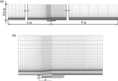
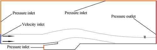
Figure 7 shows the definition of boundary conditions. The upstream boundary consists of a flow velocity inlet corresponding to the water depth and an air pressure inlet with the atmospheric pressure. The upper boundary and air vent are set as pressure inlets. The turbulence conditions at the inlets are expressed in terms of turbulence intensity level and turbulence viscosity ratio. Their embedded values in the program are 3% and 5, respectively, which is typical for flume inlet conditions (Shi, 2007). The downstream boundary is located 9 m from the deflector, where the water flow is supercritical. The boundary is positioned perpendicular to the chute base and contains both water and air. However, water depths and velocities are unknown. This is defined as a pressure outlet, denoting the free outflow of water and air. Unmentioned boundaries are treated as walls, with no-slip condition irrespective of phase. According to previous studies (e.g. Jothiprakash et al., 2015; Teng, Yang, & Pfister, 2016; Zhang et al., 2011), the RNG k-ε turbulence model is superior to other models and is used in the simulations. This model is more suited to representing free-surface turbulent flows. Unless otherwise stated, all the simulations are conducted using the modified drag-force model, in combination with the wall lubrication force model.

Figure 7. Definition of boundary conditions.

3.5. Convergence check of numerical grids

The reliability of the numerical grid was essential to our simulations. FLUENT allows one to select the discretization scheme of each governing equation. The spatial discretization of the computational domain is based on the second-order upwind scheme where higher-order levels of accuracy are achieved at cell faces. The quality of a grid is evaluated based on its density (Celik, Ghia, & Roache, 2008). Three grid resolutions are examined, namely, 18,000 cells (coarse), 31,000 cells (medium) and 52,000 cells (fine). All the grids are structured. The grid density around the aerator also increases from coarse to fine grids. Smaller cells are used at the aerator and in its vicinity. The smallest grid size of 0.5 mm is applied next to the wall boundaries.

A time-dependent procedure is applied for the solution. Iterative convergence is achieved with a decrease in normalized residuals for each equation solved by at least three orders of magnitude. The numerical formulation is fully implicit, implying that no stability criterion needs to be met in determining the time step. However, to properly model a transient flow, it is necessary to set the time step at least one order of magnitude smaller than the smallest time constant in the system. A good way to judge its choice is to observe the number of iterations needed to converge at each time step. The ideal number of iterations is 5–10 per time step. If more iterations are needed, the time step is too large and vice versa.

The parameters compared include L_m, q_a, C and Δp_a. Δp_a denotes the air-pressure drop in the air cavity. In the impingement area, the base pressure reaches a maximum value at the reattachment point, usually called as stagnation point (denoted as S). L_m refers to the cavity length, i.e. the distance along the base from the aerator offset (x = 0) to point S. Our comparisons show that the medium-sized grid generated almost identical results as those of the fine one.

Table 4 and Figure 8 show q_a values and C distributions as a function of Z = (z−z_l)/(z_u−z_l), where z_u and z_l = the upper and lower jet surfaces at C = 0.97. The location is positioned at x = 0.6 m (x/L_m = 0.21). Δp_a in the table refers to its value at the cavity centroid. Our calculations show that, given D = 1 mm, relative errors between the fine and medium grids of less than 2%. Hence, the medium-sized grid is dense enough to represent flow behaviors and is therefore used in the simulations.

Figure 8. Check of grid independence (at x = 0.6 m).

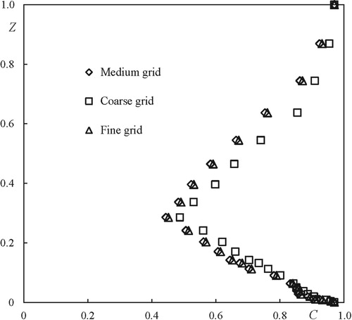
Table 4. Accuracy comparisons of three grids.

	Coarse grid	Medium grid	Fine grid
Cell number	18 000	31 000	52 000
qa (m^3/s/m)	0.324	0.374	0.375
Lm (m)	2.72	2.88	2.90
Δpa (Pa)	463	615	628

3.6. 2D modeling versus 3D modeling

The CFD results are mainly based on computations conducted in 2D. To compare and check their reliability, computations in 3D were also performed. In the 3D model, the domain had the same length as that of the 2D model; its grid had, in the x-z plane, a similar layout in terms of grid density and cell quantities. Perpendicular to the flume (y-axis with its origin; y = 0 at the chute centerline), the domain had the same width as the chute and the grid also satisfied the y⁺ criterion for the sidewalls. After our check of grid independence, the adopted grid included a total of 620,000 cells.

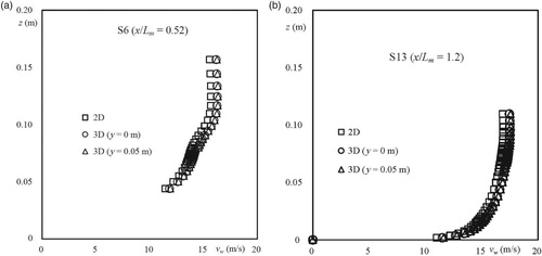
With respect to the main flow parameters, comparisons were made between them given D = 1 mm. For q_a, 2D and 3D modeling led to q_a = 0.375 and = 0.381 m³/s, respectively; the difference was only measured as 1.6%. Two typical cross-sections, one within the cavity (S6) and one in the downstream flow area (S13), were chosen to illustrate the results. Figures 9 and 10 compare the C and v_w distributions. From the 3D results, two locations, y = 0 and 0.05 m, were chosen; the corresponding results were found to be almost identical. Discrepancies between the 2D and 3D results were found to be negligibly small. Clearly, the 2D simulations generated reasonable results, which is also supported by our experimental observations. At each cross-section from S1 to S13, measurements were made at several y-locations, indicating that the sidewalls affected fewer areas than 3–4 cm from the walls and that the central part of the flow was uniform in the aerator. The experimental value of a given parameter refers to its average value based on a few measurement points in the transverse direction.

Figure 9. Comparison of C between 2D and 3D modeling.

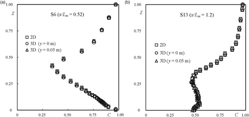
Figure 10. Comparison of v_w between 2D and 3D modeling.

4. Results and discussion

An aerator flow is conventionally divided into six zones, i.e. approach flow, transition, cavity nappe, impact, downstream flow and equilibrium flow (Figure 4) (Chanson, 1989). The reattachment point S is in the impact zone, downstream from which the base pressure head asymptotically approaches the water depth, while the near-base air concentration decreases as air bubbles detrain.

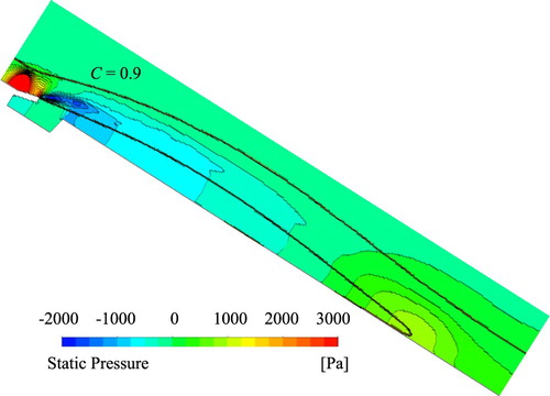
The results correspond to the steady-state solution. Even at the steady state, the flow is characterized by small perturbations. The parameters discussed below refer to their time-averaged values. To provide an overall account of the air–water flow field, Figures 11 and 12 illustrate the instantaneous flow velocity and static pressure level at the aerator. The two solid lines correspond to C = 0.90. The water flow velocity is 14.3 m/s at the offset and is 16.7 m/s at the end of the cavity. The airflow velocity amounts to 25 m/s at the upper end of the cavity and decreases toward its lower end. A slim zone of air circulation is found close to the chute base. The change in the flow direction gives rise to a local increase in water pressure at the deflector, which shifts to a negative pressure level immediately downstream as air entrainment starts. At the impact zone, the mixture also reaches a locally high pressure level.

Figure 11. Instantaneous flow velocity at the aerator.

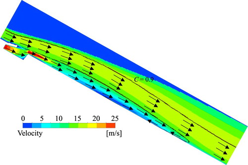
Figure 12. Instantaneous static pressure at the aerator.

The cavity configuration, airflow rate and air concentration including the rate of decay are typical parameters that describe the flow.

4.1. Cavity configuration and air-carrying capacity

In Table 5 and Figure 13, air cavity shapes and lengths derived from the tests and calculations are compared. In the table, a range is given to each parameter due to the quasi-steady nature of the flow with its mean shown in parentheses. The lack of a sharp air–water interface allows for the lower nappe boundary at C = 0.60 to represent the cavity profile as a function of x/L_m (Shi, 2007). The parameter z_m refers to the maximum value derived from the experiment (z_m = 0.051 m at x = 1.01 m). Many investigators have defined the iso-concentration line of C = 0.90 as the lower boundary. However, measurements made at locations S1, S7, S8 and S9 did not achieve this air-content level. This is why C = 0.60 is used instead.

Figure 13. Air cavity longitudinal profiles.

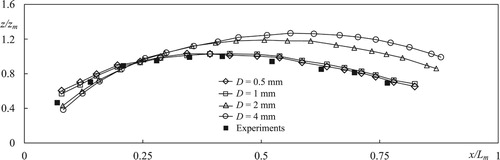
Table 5. Comparison of L_m, q_a and β between CFD and experiments.

		D (mm)
	Experiment	4	2	1	0.5
Lm (m)	2.87	3.06–3.18 (3.12)	2.90–3.04 (2.97)	2.83–2.93 (2.88)	2.84–2.91 (2.89)
qa (m^2/s)	0.375	0.38–0.42 (0.402)	0.38–0.41 (0.386)	0.35–0.39 (0.375)	0.35–0.39 (0.375)
β	0.453	0.45–0.50 (0.486)	0.45–0.49 (0.466)	0.42–0.47 (0.453)	0.42–0.39 (0.453)

One can observe deviations between the test and numerical results. The use of D = 2 and 4 mm overestimates the height and length. However, such differences are smaller when the D value decreases. It seems that both D = 0.5 and 1.0 mm give satisfactory results.

For a given q_w value, q_a reflects the air-carrying capacity of the water flow, for which a coefficient (β) is defined as β = q_a/q_w. Table 5 lists comparisons of q_a and β between the test and CFD results. Clearly, D = 2 and 4 mm somewhat overestimate the air flow; D = 0.5 and 1.0 mm provide a closer match to the test results. Despite these differences, the numerical modeling predicts the airflow well with a maximum error of less than 3% at D = 4 mm. This implies that the air-carrying capacity is not so sensitive to D.

4.2. Distributions of air concentration

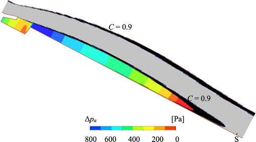
Figure 14 provides an overview of the air concentration distribution observed at the aerator. Due to the limited water depth of the approach flow, the black-water zone disappears at approximately x/L_m = 0.3. The air-pressure change in the air passage is a parameter of interest, denoting its throttling effects on the flow from the air inlet to the cavity, which are seldom observed in the literature. During the experiments, measuring Δp_a was troublesome due to the disturbance of water sprays caused by high-velocity water. The distribution of Δp_a is shown in Figure 15. The diagrams correspond to the modified model at D = 1 mm. In the simulations, the atmospheric pressure is set at the aerator’s air inlet. One can see that a maximal drop of approximately 800 Pa occurs immediately downstream from the groove. Pressure levels then recover in the flow direction. At the end of the cavity, Δp_a is only valued at approximately 100 Pa. The cavity air-pressure distribution reflects the emulsification of air into the water. With a decrease in airflow velocity in the flow direction, the air-pressure drop decreases. Although air-pressure data derived from the experiments are fragmented, they show the same trend of decline as that of the CFD model. The sharp edge in the cavity gives rise to an undesirable local pressure drop. In practical situations, the groove should be streamlined with an arc to prevent this phenomenon from occurring.

Figure 14. Overview of C distribution at the aerator (D = 1 mm).

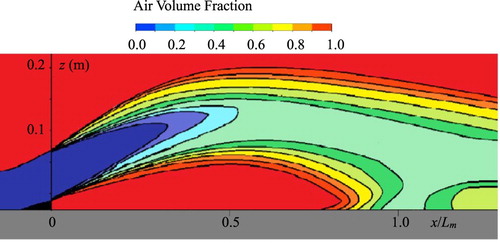
Figure 15. Air-pressure drop in the air cavity (D = 1 mm).

To compare with the experimental results, Figure 16 shows the results of the Schiller & Naumann model and of the improved model (D = 0.5, 1, 2 and 4 mm). For the former, simulations were also conducted using the four D values; the result of D = 0.5 mm is most similar to the experimental one and it is used as a reference for comparisons.

Figure 16a. C distributions at S1−S9.

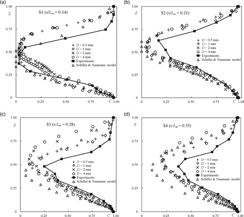
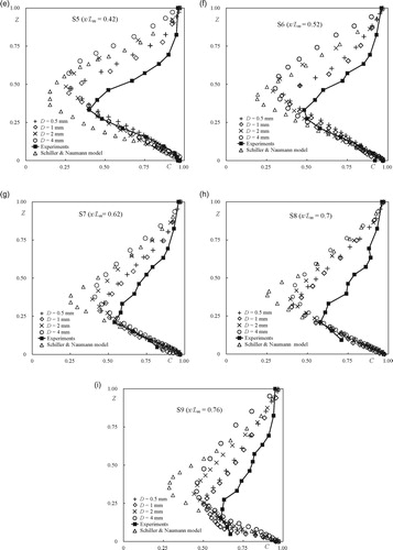
The flow shows an obvious upper and lower edge up to section S9. C distributions at S1−S9 are given in Figure 16. For the upper edge of the nappe, all of the numerical simulations underestimate the C distribution; the simulated black-water zone is somewhat longer. The modified model provides somewhat better results than the Schiller and Naumann model. C values of D = 0.5 and 1 mm are almost identical and are most similar to the experimental values. For the lower edge, the modified model produces a much better match to the experiments; results of D = 0.5 and 1 mm exhibit better agreement than those of D = 2 and 4 mm.

Sections S10 and S11 are positioned upstream from point S; S12 and S13 are positioned downstream. At these locations, the flow is confined by the chute base. Corresponding results are illustrated in Figure 17, where Z = z/z_u. Compared to those of the cavity zone, the simulated C profiles are generally more similar to the experimental profiles. The modified model makes stronger predictions than the Schiller & Naumann model and especially close to the chute base. The use of D = 0.5 and 1 mm generates almost the same results, which are in relatively good agreement with the test values.

Figure 17. C distributions at S10−S13.

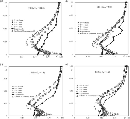
Figure 18. Comparisons of C_b between tests and CFD.

4.3. Air concentrations and downstream flow decay

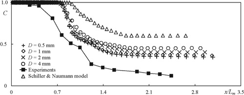
It is the dispersed air bubbles that protect the chute base from cavitation damages. It is therefore of practical significance to examine the near-wall air concentration (C_b) and its streamwise development. This provides information on the effective length of the chute provided by the aerator in question. In the experiments, air concentration transducers of resistance type were used for measurements. The transducers were placed approximately 8 mm away from the chute base. Our measurements would have been disturbed if they were placed closer.

The C_b measurements were made from the backflow in the cavity to a location at x = 7.0 m (x/L_m = 2.44). Figure 18 shows the measured results together with the simulated results. Upstream from x/L_m = 1.22, the value of C_b decreases rapidly; thereafter its gradient of decrement declines. The Schiller & Naumann model clearly overestimates the C_b profile. For the modified model, D = 0.5 and 1 mm produce almost identical profiles and generate better results than D = 2 and 4 mm. Still, C_b values from D = 0.5 and 1 mm are higher than those of the test results. Due to air detrainment, air concentrations near the base should approach zero further downstream as shown by the experiments. However, the numerical modeling generates an almost constant C_b value.

Computations of C_b are also performed for another case, i.e. an aerator at α = 30°, Δ = 10 mm and Q_w = 0.207 m³/s. Corresponding values of h₁, u₁, Q_a and F are 13.9 cm, 7.5 m/s, 105 l/s and 6.38, respectively. The simulations give rise to similar results to those shown in Figure 18; the value of C_b is also overestimated.

4.4. Effects of bubble diameters

In the Two-Fluid Model, the dispersed air component is assumed to consist of spherical air droplets or bubbles; the average size of the bubbles is represented by one constant diameter. The exchange behavior between the air and water is a dominant factor that shapes aerator flow simulations and it is influenced by the bubble size.

One can see from Equation (5) that D affects diffusion between the water and air phases; momentum exchange is more intense when D is larger. These results show that the cavity length, airflow rate and cavity pressure drop are not as sensitive to the bubble diameter; acceptable results are obtained within the diameter range examined.

For the free surface of the flow, air concentrations increase and are more similar to those of the experimental results with the decrement of D. For the cavity boundary and along the chute base, results derived from different values of D are similar; differences among them are minor.

4.5. Discussion

Regarding cavity airflow and air-concentration distributions, the modified model is superior to the Schiller and Naumann model. When impinging on the chute base, the high-velocity nappe flow forces air bubbles onto it, and this is why it is essential to include the wall-lubrication force in the model. In other industrial applications, the flow velocity is low, air bubbles do not typically travel close to solid boundaries and the effect of wall lubrication is not significant. The drag function is improved in such a way that it is based on R_r and α_a and such that it accounts for the effect of a collection of air bubbles. Still, a representative bubble diameter must be specified. The inclusion of both forces contributes to improvements in modeling accuracy. Despite this, air detrainment is still underestimated in the modified model; the near-base air concentration is overestimated and it differs from the experimental result.

This discrepancy is attributed to two sources of error: numerical and physical. The numerical procedure mainly involves domain discretization and boundary conditions. The grid is globally and locally refined to meet the grid convergence criterion. The boundary conditions are set without uncertainty. The steady aerator flow is solved as time-dependent; the iterative convergence is checked from the decrease in the residuals of equations for each time step. This numerical procedure follows best-practice guidelines of CFD modeling; contributions to discrepancies from the numerical setup should be insignificantly small.

Regarding the physics of the Two-Fluid Model, its formulation involves three other forces of air bubbles, i.e. M_l, M_td and M_vm. Coefficients are also involved in their estimation. Embedded values are used for the modeling. Sensitivity studies show that with the modified model, changing the coefficients should slightly affect results of air concentrations and cannot solely explain differences from the experiments.

In the Two-Fluid Model, air bubbles are assumed to be spherical in shape and to have no contact with one another even though the defragmentation and coalescence of bubbles occur in reality as a result of turbulent mixing. Air bubbles are rarely spherical, and this constitutes one source of error. The Two-Fluid Model also requires that the average size of dispersed air bubbles be specified by the modeler so that forces driving bubble movements relative to the surrounding water are computed. This practice is limited in that bubble sizes are not something that is already known. In addition, bubble sizes vary in both space and time across a flow field. Bubble sizes differ in the cavity and downstream flow zones.

5. Conclusions

The evaluation of two-phase flow models is essential for the prediction of entrained air in a cavity and in downstream distributions. The determination of near-base air concentrations and decay is crucial for the measurement of chute sections protected by the aerator. Experimental data derived from a test rig producing sufficiently high flow velocities render our comparisons reliable.

The Two-Fluid Model in Fluent is modified to account for the effects of drag and wall-lubrication forces. Comparisons are made with experimental data obtained from a large test rig. The following conclusions are drawn.

• The test rig produces an approach flow velocity of 14.3 m/s at the aerator, which is high enough to provide a solid basis for numerical comparisons. The tests suggest that approximately 85% of the air bubbles from the cavity fall within a mean equivalent diameter range of 0.5–4 mm.

• The modified Model considers the effects of drag and wall lubrication forces. The former refers to the effect of a collection of air bubbles on the air–water exchange behavior; the latter reflects the influence of a solid boundary on bubble movements.

• In terms of air-cavity configurations and airflow rates, smaller air bubble sizes result in a better match with the experimental data.

• With respect to cavity air concentrations, the modified model is superior to the standard version and smaller bubble diameters also give rise to better estimations.

• As far as near-base air concentrations are concerned, the modified model makes improvements. However, associated streamwise distributions are still overestimated.

The Two-Fluid Model is suited to calculations of many two-phase flow issues. However, applying an assumption of lumped single-sized spherical air bubbles is seemingly unrealistic when modeling complex flow phenomena such as aerator flows. For near-base air concentrations, differences between the CFD results and test data have indicated the limitation.

To address this limitation, more complex models such as the dynamic droplet model (e.g. FLOW-3D) or the population balance model (e.g. ANSYS) are options. Such models are based on mechanisms of the breakup of dispersed bubbles caused by shear forces and of particle coalescence resulting from flow turbulence. Air–water interactions are controlled by critical Weber and Capillary numbers. Such models contribute more realism to simulations of two-component fluid flows and should be evaluated.

Previous aerator tests have mostly focused on measurements of air concentrations in mixed flows. Attention should be dedicated to examining air bubble size spectra and corresponding time-averaged values in space in particular. Such results would undoubtedly facilitate comparisons with numerical modeling approaches. The Bubble Image Velocimetry (BIV) experimental technique identifies air-bubble breakup and coalescence patterns and should help elucidate the movement of air bubbles in aerator flows.

A prototype aerator presents similar flow behaviors to its model in terms of water–air flow parameters. When applying CFD to a prototype situation, one can reproduce airflow rates, jet trajectories and air concentration distributions in the cavity zone with confidence. However, attention must be paid to CFD results of air detrainment downstream from the impact zone and especially the decay of near-base air concentrations.

Notation

The following symbols are used in this paper:

A	=	=interfacial area (m2)
B	=	=vent height (m)
b	=	=chute width (m)
C	=	=air concentration (−)
Cb	=	=near-wall air concentration (−)
CD	=	=drag coefficient (−)
Cl	=	=lift coefficient (−)
CTD, C1ε, C2ε, Cμ	=	=constant (−)
Cw1	=	=non-dimensional coefficient (−)
Cw2	=	=non-dimensional coefficient (−)
D	=	=bubble diameter (mm)
d	=	=distance from the chute bottom (m)
F	=	=aerator Froude number (−)
f	=	=drag function (−)
G	=	=interphase force per unit volume of mixture (N/m3)
Gk,m	=	=production of turbulent kinetic energy (kg/(m·s3))
g	=	=gravitational acceleration (m/s2)
h1	=	=approaching water depth (m)
I	=	=identity tensor (−)
Kaw	=	=interphase exchange coefficient (N·s/m4)
k	=	=turbulent kinetic energy (m2/s2)
Lm	=	=jet length (m)
l	=	=chute length (m)
M	=	=interfacial force per unit volume of mixture (N/m3)
Ml	=	=lift force per unit volume of mixture (N/m3)
Mvm	=	=virtual mass force per unit volume of mixture (N/m3)
Mtd	=	=turbulence dispersion force per unit volume of mixture (N/m3)
Mwl	=	=wall-lubrication force per unit volume of mixture (N/m3)
${\stackrel{\rightharpoonup }{n}}_w$	=	=unit normal pointing away from the wall boundary
$\mathrm{\nabla }p$	=	=water-pressure gradient (N/m3)
Δpa	=	=air-pressure drop in the air cavity (Pa)
Qa	=	=air flow rate (m3/s)
qa	=	=unit air flow rate (m2/s)
Qw	=	=water flow capacity (m3/s)
qw	=	=unit water flow rate (m2/s)
R	=	=Reynolds number (−)
Rr	=	=relative Reynolds number (−)
Sk,m, Sε,m	=	=source terms (kg/(m·s3))
t	=	=physical time (s)
u1	=	=approaching flow velocity (m/s)
uτ	=	=shear velocity (m/s)
va	=	=air velocity (m/s)
vm	=	=mixture velocity (m/s)
vw	=	=water velocity (m/s)
x	=	=the x coordinate (m), parallel to the chute bottom
y	=	=the y coordinate (m), with its origin at the chute axis
ywl	=	=distance to the nearest wall boundary (m)
y+	=	=dimensionless distance from wall boundary (−)
Z	=	=dimensionless z coordinate (−)
z	=	=the z coordinate (m), perpendicular to the chute bottom
zm	=	=highest point of air cavity (measures along C = 0.60) (m)
zu	=	=upper surface of jet nappe at C = 0.97 (m)
zl	=	=lower surface of jet nappe at C = 0.97 (m)
Δ	=	=deflector height (m)
α	=	=flume bottom angle with the horizontal (°)
αa	=	=volume fraction of air (−)
αk, αε	=	=inverse effective Prandtl numbers (−)
β	=	=Air-entrainment coefficient (−)
ε	=	=turbulent dissipation rate (m2/s3)
τ	=	=shear stress (N/m2)
τa	=	=particulate relaxation time (s)
σ	=	=dispersion Prandtl number (−)
θ	=	=deflector angle with the flume (°)
ζ	=	=phase bulk viscosity (Pa·s)
μm	=	=mixture viscosity (Pa·s)
μt	=	=turbulent viscosity of the mixture (Pa·s)
μw	=	=water viscosity (Pa·s)
ρ	=	=phase density (kg/m3)
ρm	=	=mixture density (kg/m3)

Acknowledgements

The first author is indebted to Adjunct Professor Patrik Andreasson of Vattenfall R&D and Adjunct Professor Niklas Dahlbäck of Vattenfall Vattenkraft AB for support during the past decade. Ms. Sara Sandberg of the Swedish Hydropower Centre (SVC) is acknowledged for project co-ordinations with the Royal Institute of Technology (KTH) and Vattenfall R&D.

Disclosure statement

No potential conflict of interest was reported by the authors.

ORCID

James Yang http://orcid.org/0000-0002-4242-3824

Additional information

Funding

The study was carried out as part of a research project entitled ‘Hydraulic design of chute spillway aerators’, funded by the Swedish Hydropower Centre (SVC). SVC has been established by the Swedish Energy Agency, Energiforsk AB and Swedish National Grid (Svenska Kraftnät), together with Royal Institute of Technology (KTH), Luleå University of Technology (LTU), Chalmers University of Technology (CTH) and Uppsala University (UU). The experiments were performed by Institute of Water Resources and Hydropower Research (IWHR), Beijing.

References

- ANSYS. (2015). Help system, fluent multiphase flows theory guide. (Academic Research Release 15). Canonsburg: ANSYS Inc.
- Antal, S. P., Lahey, R. T., & Flaherty, J. E. (1991). Analysis of phase distribution in fully developed laminar bubbly two-phase flow. International Journal of Multiphase Flow, 17(5), 635–652. doi: 10.1016/0301-9322(91)90029-3
- Aydin, M. C., & Ozturk, M. (2009). Verification and validation of a computational fluid dynamics (CFD) model for air entrainment at spillway aerators. Canadian Journal of Civil Engineering, 36(5), 826–836. doi: 10.1139/L09-017
- Bai, R., Zhang, F., Liu, S., & Wang, W. (2016). Air concentration and bubble characteristics downstream of a chute aerator. International Journal of Multiphase Flow, 87, 156–166. doi: 10.1016/j.ijmultiphaseflow.2016.07.007
- Celik, I. B., Ghia, U., & Roache, P. J. (2008). Procedure for estimation and reporting of uncertainty due to discretization in CFD applications. Trans ASME Journal of Fluids Engineering, 130(7), 078001-1–078001-4.
- Chanson, H. (1989). Study of air entrainment and aeration devices. Journal of Hydraulic Research, 27(3), 301–319. doi: 10.1080/00221688909499166
- Chanson, H. (1994). Aeration and deaeration at bottom aeration devices on spillways. Canadian Journal of Civil Engineering, 21(3), 404–409. doi: 10.1139/l94-044
- Chanson, H. (1997). Air bubble entrainment in free-surface turbulent shear flows. Brisbane: Academic Press.
- Chanson, H., & Lubin, P. (2010). Discussion of ‘verification and validation of a computational fluid dynamics (CFD) model for air entrainment at spillway aerators’ appears in the Canadian journal of civil engineering 36(5): 826–838. Canadian Journal of Civil Engineering, 37(1), 135–138. doi: 10.1139/L09-133
- Chanson, H., & Toombes, L. (2002). Air-water flows down stepped chutes: Turbulence and flow structure observations. International Journal of Multiphase Flow, 28, 1737–1761. doi: 10.1016/S0301-9322(02)00089-7
- Chau, K. W., & Jiang, Y. W. (2001). 3D numerical model for Pearl River estuary. Journal of Hydraulic Engineering, 127(1), 72–82. doi: 10.1061/(ASCE)0733-9429(2001)127:1(72)
- Chau, K. W., & Jiang, Y. W. (2004). A three-dimensional pollutant transport model in orthogonal curvilinear and sigma coordinate system for Pearl river estuary. International Journal of Environment and Pollution, 21(2), 188–198. doi: 10.1504/IJEP.2004.004185
- Crawford, T. J., Weinberger, C. B., & Weisman, J. (1985). Two-phase flow patterns and void fractions in downward flow part I: Steady-state flow patterns. International Journal of Multiphase Flow, 11(2), 761–782. doi: 10.1016/0301-9322(85)90023-0
- Crawford, T. J., Weinberger, C. B., & Weisman, J. (1986). Two-phase flow patterns and void fractions in downward flow. Part II: Void fractions and transient flow patterns. International Journal of Multiphase Flow, 12(2), 219–236. doi: 10.1016/0301-9322(86)90027-3
- Deng, J., Xu, W. L., Lei, J., & Diao, M. J. (2005). Numerical simulation of hydraulic characteristics of high head spillway tunnel. Chinese Journal of Hydraulic Engineering, 36(10), 1209–1212. (in Chinese).
- Drew, D. A., & Lahey, R. T. (1993). In particulate two-phase flow. Boston: Butterworth-Heinemann.
- Ekambara, K., Dhotre, M. T., & Joshi, J. B. (2005). CFD simulations of bubble column reactors: 1D, 2D and 3D approach. Chemical Engineering Science, 60(23), 6733–6746. doi: 10.1016/j.ces.2005.05.047
- Falvey, H. T. (1980). Air-water flow in hydraulic structures. Engineering Monograph 41. Denver: United States Department of the Interior, Bureau of Reclamation.
- Falvey, H. T. (1990). Cavitation in chutes and spillways. Engineering Monograph 42. Denver: United States Department of the Interior, Bureau of Reclamation.
- Greifzu, F., Kratzsch, C., Forgber, T., Lindner, F., & Schwarze, R. (2016). Assessment of particle-tracking models for dispersed particle-laden flows implemented in OpenFOAM and ANSYS FLUENT. Engineering Applications of Computational Fluid Mechanics, 10(1), 30–43. doi: 10.1080/19942060.2015.1104266
- Hibiki, T., & Ishii, M. (2000). One-group interfacial area transport of bubbly flows in vertical round tubes. International Journal of Heat and Mass Transfer, 43(15), 2711–2726. doi: 10.1016/S0017-9310(99)00325-7
- Hirt, C. W., & Nichols, B. D. (1981). Volume of fluid (VOF) method for the dynamics of free boundaries. Journal of Computational Physics, 39(1), 201–225. doi: 10.1016/0021-9991(81)90145-5
- ICOLD. (1987). Dam safety guidelines. Bulletin No. 59. Paris: International Committee on Large Dams.
- ICOLD. (1992). Selection of design flood - current methods. Bulletin No. 82. Paris: International Committee on Large Dams.
- Ishii, M., & Mishima, K. (1984). Two-fluid model and hydrodynamic constitutive relations. Nuclear Engineering and Design, 82(2), 107–126. doi: 10.1016/0029-5493(84)90207-3
- Ishii, M., & Zuber, N. (1979). Drag coefficient and relative velocity in bubbly, droplet or particulate flows. AIChE Journal, 25(5), 843–855. doi: 10.1002/aic.690250513
- Joshi, J. B. (2001). Computational flow modelling and design of bubble column reactors. Chemical Engineering Science, 56(21), 5893–5933. doi: 10.1016/S0009-2509(01)00273-1
- Jothiprakash, V., Bhosekar, V. V., & Deolalikar, P. B. (2015). Flow characteristics of orifice spillway aerator: Numerical model studies. ISH Journal of Hydraulic Engineering, 21(2), 216–230. doi: 10.1080/09715010.2015.1007093
- Kökpınar, M. A., & Göğüş, M. (2002). High-speed jet flows over spillway aerators. Canadian Journal of Civil Engineering, 29(6), 885–898. doi: 10.1139/l02-088
- Kolev, N. I. (1977). Two-phase two-component flow (air-water steam-water) among the safety compartments of the nuclear power plants with water cooled nuclear reactors during loss of coolant accident ( PhD Thesis). Technical University Dresden, Germany.
- Kolev, N. I. (2005). Multiphase flow dynamics 2. Thermal and mechanical interactions (2nd ed.). Berlin: Springer-Verlag.
- Kramer, K. (2004). Development of aerated chute flow (Ph.D. dissertation). Versuchsanstalt für Wasserbau, Hydrologie und Glaziologie, ETH, Zurich, Switzerland.
- Kramer, K., & Hager, W. H. (2005). Air transport in chute flows. International Journal of Multiphase Flow, 31(10), 1181–1197. doi: 10.1016/j.ijmultiphaseflow.2005.06.006
- Liu, T., & Yang, J. (2014). Three-dimensional computations of water–air flow in a bottom spillway during gate opening. Engineering Applications of Computational Fluid Mechanics, 8(1), 104–115. doi: 10.1080/19942060.2014.11015501
- Matos, J., & Frizell, K. H. (1997). Air concentration measurements in highly turbulent aerated flow. 27th IAHR congress, San Francisco, USA.
- Michaelides, E. E. (2003). Hydrodynamic force and heat/mass transfer from particles, bubbles, and drops—The freeman scholar lecture. Journal of Fluids Engineering, 125(2), 209–238. doi: 10.1115/1.1537258
- Moraga, F. J., Bonetto, R. T., & Lahey, R. T. (1999). Lateral forces on spheres in turbulent uniform shear flow. International Journal of Multiphase Flow, 25(6), 1321–1372. doi: 10.1016/S0301-9322(99)00045-2
- Orszag, S. A., Yakhot, V., Flannery, W. S., Boysan, F., Choudhury, D., Maruzewski, J., & Patel, B. (1993). Renormalization group modeling and turbulence simulations. International conference on near-wall turbulent flows, Tempe, USA.
- Owen, G. D., & Hewitt, G. F. (1987). An improved annular two-phase flow model. 3rd BHRA Int. Conf. On multiphase flow, Hague, Netherlands.
- Özkan, F., Wenka, A., Hansjosten, E., Pfeifer, P., & Kraushaar-Czarnetzki, B. (2016). Numerical investigation of interfacial mass transfer in two phase flows using the VOF method. Engineering Applications of Computational Fluid Mechanics, 10(1), 100–110. doi: 10.1080/19942060.2015.1061555
- Pfister, M., & Hager, W. H. (2010a). Chute aerators. I: Air transport characteristics. Journal of Hydraulic Engineering, 136(6), 352–359. doi: 10.1061/(ASCE)HY.1943-7900.0000189
- Pfister, M., & Hager, W. H. (2010b). Chute aerators. II: Hydraulic design. Journal of Hydraulic Engineering, 136(6), 360–367. doi: 10.1061/(ASCE)HY.1943-7900.0000201
- Pinto, N. L. S., Neidert, S. H., & Ota, J. J. (1982). Aeration at high velocity flows. Water Power and Dam Construction, 34(2), 34–38.
- Rahimzadeh, H., Maghsoodi, R., Sarkardeh, H., & Tavakkol, S. (2012). Simulating flow over circular spillways by using different turbulence models. Engineering Applications of Computational Fluid Mechanics, 6(1), 100–109. doi: 10.1080/19942060.2012.11015406
- Schiller, L., & Naumann, Z. (1935). A drag coefficient correlation. Zeitschrift des Vereins Deutscher Ingenieure, 77, 318–320.
- Schlichting, H., & Gersten, K. (2000). Boundary-layer theory (8th revised ed.). Berlin: Springer-Verlag.
- Shi, Q. S. (2007). High-velocity aerated flow. Beijing: China Water & Power Press. (in Chinese).
- Simonin, O., & Viollet, P. L. (1990). Modeling of turbulent two-phase jets loaded with discrete particles. In Phenomena in multiphase flows (pp. 259–269). Washington, DC: Hemisphere Publishing Corporation.
- Sokolichin, A., Eigenberger, G., & Lapin A. (2004). Simulation of buoyancy driven bubbly flow: Established simplifications and open questions. AIChE Journal, 50(1), 24–45. doi: 10.1002/aic.10003
- Stokes, G. G. (1880). Mathematical and physical papers. London: Cambridge University Press.
- Tabib, M. V., Roy, S. A., & Joshi, J. B. (2008). CFD simulation of bubble column—An analysis of interphase forces and turbulence models. Chemical Engineering Journal, 139(3), 589–614. doi: 10.1016/j.cej.2007.09.015
- Teng, P., Yang, J., & Pfister, M. (2016). Studies of two-phase flow at a chute aerator with experiments and CFD modelling. Modelling and Simulation in Engineering, 2016, 1–11. Article ID 4729128, doi: 10.1155/2016/4729128
- Volkart, P., & Rutschmann, P. (1984). Rapid flow in spillway chutes with and without deflectors – a model-prototype comparison. Proc. Symp. On scale effects in modelling hydraulic research, Esslingen, Germany.
- Wood, I. R. (Ed.). (1991). Air entrainment in free-surface flows. Rotterdam: A.A. Balkema.
- Wu, C. L., & Chau, K. W. (2006). Mathematical model of water quality rehabilitation with rainwater utilization: A case study at Haigang. International Journal of Environment and Pollution, 28(3–4), 534–545. doi: 10.1504/IJEP.2006.011227
- Xu, W. L., Wang, W., Tan, L. X., & Yang, Y. Q. (2001). Numerical simulation of air-water two-phase flows in hydraulic engineering. Chinese Journal of Hydrodynamics, 16(2), 226–230. (in Chinese).
- Zhang, J. M., Chen, J. G., & Xu, W. L. (2011). Three-dimensional numerical simulation of aerated flows downstream sudden fall aerator expansion-in a tunnel. Journal of Hydrodynamics, Ser. B, 23(1), 71–80. doi: 10.1016/S1001-6058(10)60090-X
- Zhang, H. W., Liu, Z. P., Zhan, D., & Wu, Y. H. (2008). Numerical simulation of aerated high velocity flow downstream of an aerator. Chinese Journal of Hydraulic Engineering, 39(12), 1302–1308. (in Chinese).