CFD modeling as part of a hybrid modeling case study for a gauging station with challenging hydraulics

ABSTRACT

Estimates of peak flood discharges are most often based on stage measurements, and the discharge is determined indirectly from the extrapolation of a rating-curve. It is possible to improve the extrapolation of the rating-curve by hydraulic modeling, such as scale or numerical models. In this paper, we discuss a case study for a streamflow gauging station in a mountainous river in Norway. A computational fluid dynamics model is used as part of a hybrid modeling study to study the flow at this gauging station with challenging geometry and flow and derive a reliable rating-curve. The numerical model produces stage-discharge data with comparable accuracy to the scale model. Analysis of the results of the hybrid modeling shows that the original location of stage measurements is not suitable for field measurements or for modeling the rating curve. Based on the modeling, an alternative point of measurement with better flow conditions at high flows is identified. The results and findings highlight the importance of 3-dimensional flow at the site during floods and shows how computational fluid dynamics can be used to provide stage-discharge data for rating curves and provide additional insight in hybrid modeling.

KEYWORDS:

• CFD
• numerical simulation
• hybrid modeling
• free-surface flow
• rating curve
• gauging station

Introduction

To know the uncertainty in river flood discharges from rating-curves is important for many applications, for example for determining design-floods by flood frequency analysis (Steinbakk et al., 2016) and calibrating rainfall-runoff models or hydraulic models (Domeneghetti, Castellarin, & Brath, 2012). During flood events, the river usually experiences velocities too high for safe measurement of discharge, and it can also be logistically challenging to capture peak floods in remote catchments. For these reasons, corresponding discharges for the highest measured stages during floods are usually not available, and the rating-curve is often extrapolated to obtain an estimate of the flood discharge. Efforts have been made to quantify the extrapolation error in rating curves. For example, in Petersen-Øverleir, Soot, and Reitan (2008), 581 Norwegian gauging stations were assessed using Bayesian interference. Around a quarter of the stations were found to have uncertainty larger than 40% for high flows. In Italy, G. Di Baldassarre and Montanari (2009) found an average high flow extrapolation error for a reach in the river Po to be 14%. The extrapolation error will also typically increase with higher discharges (Di Baldassarre, Laio, & Montanari, 2012; Kuczera, 1996).

The conditions that determine the stage at the gauging station is termed the hydraulic control. This control can be an artificial structure or natural features. In the literature, the hydraulic control is usually classified as either a channel control or section control (Herschy, 2009; Rantz, 1982; WMO, 2010). A section control is a section where the flow passes through super-critical, and the capacity of the section solely determines the stage upstream. For example, the section can be an artificial weir, or a rapid or contraction in natural rivers. A channel control is a relatively homogenous stretch of the river that determines the stage. The flow conditions are usually sub-critical within this stretch. The hydraulic control is often further classified as a compound control if a combination of several partial controls exists, or as a complete control if only one control determines the stage (WMO, 2010).

Usually, only the stage (h) is continually monitored at the gauging station and the discharge (Q) is estimated from a pre-determined stage-discharge relationship or rating-curve based on a sample of direct discharge measurements, often only obtained during lower flow conditions. The river-stage measurement is often an estimate based on a measured pressure (p) giving a hydraulic head (ψ) in a stilling well. The stage in the river is assumed to be approximately equal to the hydraulic head by assuming a hydrostatic pressure distribution. Most often, the rating function is assumed to follow a power-law relationship, on the form (e.g. Dymond & Christian, 1982): (1) $Q=C(h-h_0{)}^{\wedge }b$(1) where h₀ is the stage of zero flow, C is a coefficient and b are an exponent that must be determined. Multiple segments of power-law functions can be considered, and a power-law based rating function with multiple segments can be expressed (Reitan & Petersen-Overleir, 2009): (2) $\begin{array}{rl}Q& =0\mathrm{for}h<h_{01}\\ Q& =C_1(h-h_{01}{)}^{\wedge }{b}_1\text{for}{h}_{01}<h<h_{s1}\\ Q& =C_n(h-h_{0n}{)}^{\wedge }{b}_n\text{for}{h}_{\text{sn}-1}<h<h_{sn}\end{array}$(2)

Here h₀₁ is the actual stage of zero flow, for example the elevation of the lowest point in the section in the case of a section control. h_0n is the theoretical stage of zero flow for all segments higher than the first one. h_sn is the threshold between segment n and segment n−1, C_n is the coefficient, and b_n is the slope of the rating function for segment n. A classical method for fitting power-law functions to stage-discharge data is by the log–log method (Herschy, 2009; WMO, 2010). For example, Bayesian methods (Moyeed & Clarke, 2005) can also be used to estimate the rating curve parameters and their uncertainty. Such methods can also be utilized for segmented formulations (Reitan & Petersen-Overleir, 2009).

Hydraulic models, such as models based on the 1- or 2-dimensional St. Venant equations, can be applied to obtain rating curves, and decrease the uncertainty in the extrapolation or interpolation of rating curves (some examples are Abril & Knight, 2004; Corato, Moramarco, & Tucciarelli, 2011; Di Baldassarre & Claps, 2011; Domeneghetti et al., 2012; Shao, Dutta, Karim, & Petheram, 2018; Yang, Ho, Hwang, & Lin, 2014). Such models make simplifying assumptions about hydraulic conditions in the river (see e.g. Novak, Guinot, Jeffrey, & Reeve, 2010). In 1-dimensional models, the stage and velocity must be assumed to be uniform over the river section. In many cases, the stage will vary transversally over the river. Non-uniform flow in the vertical or transversal direction over the river-section can also cause the stage to vary. 2-dimensional models take lateral velocities and changes in water levels into account, but still neglect the vertical velocity component and in most cases operate under a hydrostatic pressure assumption.

Non-uniform flow, varying stage and other problems such as high velocities can be mitigated by finding a good site for stage measurements, for example following the guidelines given in WMO (2010), however it is well known that such conditions are often not found in practice, and consequently the assumptions made in 1- or 2-dimensional models may not always hold. During floods, the conditions for stage measurements will often be particularly adverse due to high velocities and wave production in the river. In cases where non-hydrostatic pressure components or verticality in the flow field is important, 3-dimensional non-hydrostatic computational fluid dynamics (CFD) models are necessary to give a good description of the flow (e.g. Novak et al., 2010).

In hydraulic engineering, a combination of CFD models with hydraulic scale modeling is often used (Bermúdez et al., 2017; Hager & Boes, 2014). This approach, often termed hybrid modeling, is advantageous because of the complementing properties of these two hydraulic modeling methods. An advantage in hybrid modeling is that once the CFD model is validated against the scale model, it can be used to provide additional insight, for example by giving detailed information about the flow field and water surface, which can be difficult to obtain from the scale model. Even with current advances in instrumentation techniques, such as particle imaging velocimetry (PIV) and Acoustic Doppler Velocimetry (ADV), the recording of even single point measurements of velocity or pressure can be relatively laborious. In contrast, once a CFD model has been set up and run, pressures, velocity vectors and turbulent properties for each computational node is readily available. The CFD model further provides the advantage that large changes to the model geometry can be made with relative ease, and different scenarios can be tested. Scale models are however sometimes the better choice for making quick, smaller changes to the model on the fly and can be better for getting a first impression of the problems arising, as an experiment can be conducted within hours or minutes. Finally, scale models are subject to scale effects (e.g. Heller, 2011). Careful modeling, and knowledge about the problem allows hydraulic engineers to circumvent problems of scale. However, for free surface flow, particularly aeration and surface tension effects can be important issues, and in the case of super critical or aerated flows, obtaining data from the scale models becomes even more challenging (see Hager & Boes, 2014 and references within). While no scale effects have to be considered in the field of CFD, adequate modeling of for instance air entrainment and aerated flows remains a challenging task also in CFD (e.g. Lopes, Tabor, Carvalho, & Leandro, 2016).

The available computational resources for CFD have been increasing rapidly. This is due to both the development in hardware and high-performance computing but also due to more efficient algorithms and mesh generation (Slotnick et al., 2014). Consequently, methods relying on very fine computational meshes such as Large eddy simulation (LES) and detached eddy simulation (DES) are also becoming more viable. Some recent examples in hydraulic engineering are LES of flow through submerged bridge openings (Kara, Stoesser, Sturm, & Mulahasan, 2015) and DES of skimming flow over a stepped spillway (Toro, Bombardelli, & Paik, 2017). Meshless methods for hydraulic engineering are also becoming more viable, for example based on smoothed particle hydrodynamics (Amicarelli, Kocak, Sibilla, & Grabe, 2018; Wan, Li, Pu, Zhang, & Feng, 2018).

However, the most common approach to CFD in hydraulic engineering as well as other fields have been based on the Reynolds-Averaged Navier Stokes (RANS) equations. Even if the accuracy of RANS models is lower compared to LES and DNS, an advantage is the balance between computational cost and accuracy which make them popular, especially for industrial applications. RANS models have been successfully deployed to model the stage-discharge relationship for hydraulic structures for the last decades, for example for round-crested weirs and spillways (Dargahi, 2006; Gessler, 2005; Kirkgoz, Akoz, & Oner, 2009; Olsen & Kjellesvig, 1998; Pedersen, Fleit, Pummer, Tullis, & Rüther, 2018; Savage & Johnson, 2001; Zeng, Zhang, Ansar, Damisse, & González-Castro, 2016a, 2016b), broad-crested weirs (Hargreaves, Morvan, & Wright, 2007; Haun, Olsen, & Feurich, 2011; Sarker & Rhodes, 2004), and compound channels (Conway, O'Sullivan, & Lambert, 2013) among many other applications for hydraulic engineering. While several of these studies compare RANS model to hydraulic scale model results, they were not developed as part of a hybrid modeling approach. A recent example of a hybrid modeling study for the intake-outlet of a pumped-storage hydropower plant can be found in Bermúdez et al. (2017).

In the current study, a 3-dimensional RANS model with conventional turbulence closure is employed as part of a hybrid modeling approach to study the flow pattern at the Eggafossen gauging-station. Eggafossen is located in a mountainous river in central Norway. To the authors’ knowledge, the case study contributes to the current research state-of-the-art on CFD modeling of rating curve in two ways. Firstly, while RANS models have been applied to model rating relationships before (see above), the presented method and results increase the knowledge in the application of RANS models to model rating curves for natural gauging stations with a high level of complexity in geometry and flow. The second novelty within this paper is the successful application of a hybrid modeling approach to gauging stations. Sensitivity tests on the roughness parameter indicated that while the location of the current gauging station is sensitive to the roughness at high flows, other points that was found more suitable for stage measurement where not sensitive to the roughness parameter. Therefore, no calibration of a roughness number was necessary in either the scale model or the CFD model for these points. This is likely due to the water level being governed mainly by a critical section type control at these points, as opposed to the current gauging station location were the flow is disturbed due to an obstruction.

The current hybrid modeling case study was first described in conference proceedings presenting limited, preliminary results (Pedersen & Rüther, 2016). This paper presents the full results, including an expanded CFD model. The gauging-station in the study belongs to the Norwegian Water Resources and Energy directorate (NVE) and is located upstream of a waterfall formed by natural bedrock weir. The geometry and inflow conditions at the site cause difficult conditions for stage-measurement that warrant the use of modeling the full 3-dimensional flow field. The first goal of the study is to validate the CFD model against a recent scale model study (Pedersen, Aberle, & Rüther, 2018). Once the model is validated, the second goal of the study is to expand the geometry in the CFD model to study the flow outside of the original study area in the scale model. The CFD model allows for additional insight compared to the scale model by obtaining detailed flow fields and water surface elevation output. The CFD model capability for assessing the suitability for stage measurements at sites with difficult measurement conditions is demonstrated, and stage-discharge data for an alternative rating-curve for high flows is produced.

Hybrid modeling method

Hydraulic scale model study

The present case study site is a gauging station located in the Gaula river in central Norway. The gauging station site was reproduced in a hydraulic scale model study at the Norwegian hydrotechnical laboratory in 2016–2017 (Pedersen, Aberle, et al., 2018). A computer numerical control (CNC) machining technique was utilized to obtain an accurate representation of an approximate 150 × 75 m area of the river in non-distorted length scale 1:17.5. The scale model was used to analyze problems with the gauging station rating curve and demonstrated the use of a scale model to provide synthetic data for a rating-curve for high flows. In order to provide stage-discharge data for the rating-curve, the hydraulic head and water surface elevation was measured in several points in the model between 7.5 and 650 m³ s⁻¹ discharges. A field survey utilizing a combination of terrestrial laser scans, total station and sonar measurements provided the data for a 3-dimensional surface description of the site.

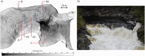
Figure 1(a) shows the plan view of the geometry of the Eggafossen site and the measurement points (A, A2, B, B2, C and GS) used in the study. In the field, measurements of stage are conducted in the pool upstream from a waterfall where a rock outcrop forms a natural bedrock weir (Figure 1(b)). The waterfall exerts full or partial hydraulic control for the gauging station for all considered discharges. At mean discharge, a level pool with low velocities forms upstream of the rock outcrop, giving good measurement conditions. The flow into this pool comes in through a rapid, and upstream of the rapid there is a long curve (upstream of the geometry shown in Figure 1(a)). Point GS is located at the current field stage measurement location. Points A and A2 are located along the thalweg of the river and point B and B2 are located on the left side. Cross sections where ADV measurements are available from the scale model are also indicated in Figure 1(a) (CS-1 and CS-2). In the field, the stage is measured in a stilling well connected to point GS. The mean discharge at the site, considering the years 1961–1990, is 17 m³s⁻¹, while the mean annual flood is 221 m³ s⁻¹.

Figure 1. (a) Eggafossen geometry (prototype scale), measurement points and location of cross sections for velocity measurement (dotted lines). The flow direction is from left to right. Contour lines are 1 m equidistant; (b) photo of the Eggafossen waterfall from downstream.

CFD model setup

Governing equations

A goal of this study was to select a numerical model that can also be employed with the resources available in an industrial setting. Therefore, the numerical model is set up using formulations that are fairly standard in use and available today in major commercial or open source CFD software such as Flow-3D (‘Flow-3D [Computer software]’, n.d.) STAR CCM+ (‘STAR-CCM+ version 10.02 [Computer software]’, n.d.), and OpenFOAM (‘OpenFOAM [Computer software]’, n.d.). The commercial CFD software STAR CCM+ is used for modeling in the present study.

The problem at hand involves a free-surface two-phase water and air flow. The governing equations are the (Unsteady) Reynolds-Averaged Navier-Stokes (RANS) equations for incompressible flow: (3) $\frac{\mathrm{\partial }{\overline{u}}_i}{\mathrm{\partial }{x}_i}=0$(3) (4) $\begin{array}{rl}& \frac{\mathrm{\partial }{\overline{u}}_i}{\mathrm{\partial }t}+{\overline{u}}_j\frac{\mathrm{\partial }{\overline{u}}_i}{\mathrm{\partial }{x}_j}={\overline{f}}_i\\ & +\frac{1}{\rho }\left[-\frac{\mathrm{\partial }\overline{p}}{\mathrm{\partial }{x}_i}+\frac{\mathrm{\partial }}{\mathrm{\partial }{x}_j}\left(\mu \frac{\mathrm{\partial }{\overline{u}}_i}{\mathrm{\partial }{x}_j}-\rho \overline{{u^{\prime }}_i{u^{\prime }}_j}\right)\right]\left(5\right)\end{array}$(4)

The RANS equations are discretised and solved using a finite volume method (see e.g. Versteeg & Malalasekera, 2007). The Volume of Fluid (VOF) method (Hirt & Nichols, 1981) is used to track the volume fractions of water and air by solving an additional transport equation. A High-Resolution Interface Capturing (HRIC) discretization scheme is used for the VOF transport equation, in order to avoid smearing of the free-surface interface. The Reynolds-stress term, $-\rho \overline{{u^{\prime }}_i{u^{\prime }}_j}$, in Equation (4) appears due to the Reynolds-Averaging and can be approximated using a turbulence model. Realizable k-epsilon (RKE) model (Shih, Liou, Shabbir, Yang, & Zhu, 1995) is used for modeling the Reynolds stress term. The RKE turbulence involves solving additional transport equations for k and epsilon. Both the RANS equations and the RKE transport equations are discretised using 2nd-order convection schemes. Further information about the numerical methods mentioned, can be found in the STAR CCM+ documentation (CD-adapco, 2015).

Geometry and meshing

Scale models are often limited in their spatial extension as result of the combination of choice of scale and the available space. One big advantage of the hybrid modeling approach is the possibility to expand the geometry in the CFD model. In the present study, the geometry is expanded in the CFD model to also incorporate the flow upstream of the pool. Two different CFD model geometries are therefore used in this study. First, the same geometry used in the scale model is used in order to validate the CFD model. A larger, expanded geometry is then used for the consecutive flow analysis and extraction of stage-discharge data for a rating-curve.

The computational mesh used in this study utilizes cells of arbitrary polyhedral shape, rather than the more commonly used tetrahedral or hexahedral cell shapes. Figure 2 shows the final mesh of the expanded model and an indication of the borders for the shorter, original model. Larger cells are used for the upstream curve as well as downstream of the bedrock weir (0.2 m). A finer mesh resolution is used in the upstream pool (0.025 m) and the ridge at the edge of the fall (0.01 m). The total number of cells is approximately 1 million for the final mesh.

Figure 2. Computational mesh for the CFD model plotted at surface. The dotted box indicates borders for the short model. Flow is from left to right.

Initial and boundary conditions

Discharges between 7.5 and 650 m³ s⁻¹ are run in the CFD model. A uniform velocity field is defined normal to the inlet to obtain a fixed mass flux that corresponds to the desired discharge. The water surface elevation is also set at the inlet by defining the volume fraction of water and air.

The downstream boundary is set to an atmospheric pressure condition. Physically, this means that no backwater effect from downstream boundary is accounted for in the simulations. For most flows, the area of interest is not influenced by the downstream boundary, because there is super-critical flow over the bedrock weir. However, for higher flows the bedrock weir becomes partially submerged, and it is then assumed that the shallow contraction will act as the control for the tail-water, and not the downstream boundary. The top boundary is also set to atmospheric pressure. The geometry itself is set to a no-slip boundary condition with a smooth or rough wall formulation. For rough wall formulations, roughness heights k_s = 0.001–0.005 m are used. The simulations are run with constant discharge at the inlet until the in and out flux of the model is in balance and quasi-steady state conditions are reached. A time step of 0.001 s was used.

Validation and sensitivity

CFD model validation

The first phase of CFD modeling in the hybrid modeling approach is to validate the CFD model against scale model results. In this phase, the same 3-dimensional stereolithographic (STL) geometry file that is used as input for the scale model is also used as input for the CFD model. The final CFD and scale model geometries should therefore be in close agreement, only neglecting errors introduced by machining and surface treatment of the scale model, and the approximation of the surface used for meshing in the numerical model. Six point-measurements of hydraulic head or water surface elevations in the scale model are compared to corresponding points (A, A2, … in Figure 1(a)) in the CFD model for the range of considered discharges (7.5–650 m³ s⁻¹). Hydraulic heads are measured in the scale model by hydraulically connected stilling wells and the water surface elevation is measured using ultrasonic sensors or needle gauge (see Pedersen, Aberle, et al., 2018). In addition, ADV measurements from the scale model at discharge of 7.5 and 300 m³ s⁻¹ are compared to the simulated velocity field in the CFD model in two cross-sections (CS-1 and CS-2 in Figure 1(a)).

Figure 3 shows the hydraulic head recorded in the numerical model (CFD) compared to hydraulic heads (HSM) and water surface elevations (WL HSM) measured in the scale model. Water surface elevation is used for comparison for point A2 and B2 and partially for point C since measurements of hydraulic heads were not available from the scale model. Deviations at these points may consequently be due to non-hydrostatic pressures, however the deviations at these points are small. It can be observed from Figure 3 that the largest deviation between the CFD and scale model is found at point GS and point A. For point GS, it is observed in both the scale model and CFD model, that a rock outcrop obstruction upstream causes challenging conditions for discharges > 100 m³ s⁻¹ (details in Pedersen, Aberle, et al., 2018). In particular, the water surface gradient and non-hydrostatic conditions at the point makes it unsuitable both with regard to modeling and for measurements in the field. The simulated flow field around and in the wake of the obstruction causing challenging conditions at point GS is shown in Figure 4 at 300 m³ s⁻¹. Sensitivity tests show that the measured hydraulic head is very sensitive to the exact point of measurement, due in part to a large transversal gradient in the water surface elevation forming at this point. Measurements at point A is also somewhat disturbed because of these effects. In addition, the rapid upstream is observed to cause standing waves that might also have affected the measurements. Other than these discrepancies, the CFD model produces stage-discharge data in reasonable agreement with the scale model for all the other points, as seen in Figure 3.

Figure 3. Stage-discharge data comparison between CFD model and hydraulic scale model (HSM).

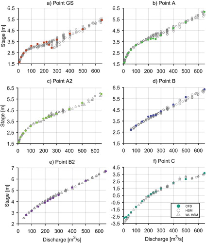
Figure 4. Near surface velocity vectors for a discharge of 300 m³ s⁻¹, showing the triangulated surface geometry and flow field around the rock outcrop and 3-dimensional roller structure in the wake close to point GS.

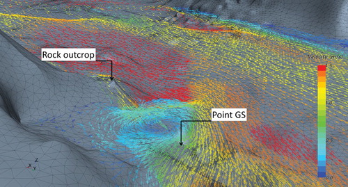
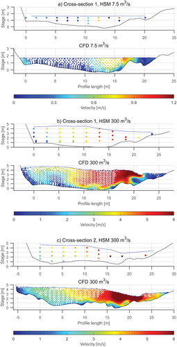
Figure 5 shows the ADV measurement points in the scale model and corresponding velocities in the CFD model. The ADV measurements were done in cross-section 1 for 7.5 m³ s⁻¹ discharge, and in cross-section 1 and 2 for 300 m³ s⁻¹ discharges. The cross-section geometry and water surface elevations, as measured with needle gauge, are also plotted. The velocity profiles can be observed to be in good agreement regarding the location of the main currents. For example, at 7.5 m³ s⁻¹ (Figure 5(a)), the largest velocities occur 11–18 m from the left bank with a maximum velocity of ∼1 m s⁻¹. Also, a slight increase in velocities along the left bank can be observed in both the physical and numerical model (Figure 5(a)). Similarly, reasonable agreement can be observed for the 300 m³ s⁻¹ cases (Figure 5(b,c)). Apart from the broad agreement, there are some differences in details. For example, in Figure 5(b) on the right side (x = 21 m) the numerical model shows a field of low velocity that does not seem to be reflected in the ADV measurements. This is due to disturbances in the wake of the obstruction at point GS seen in Figure 4. At 7.5 m³ s⁻¹ the water surface is flat in the transversal direction, and in agreement between the scale model and CFD model (Figure 5(a)). At 300 m³ s⁻¹, there is significant draw-down of the water surface on the right side of both cross-sections, seen in both the scale model and the CFD model. For section 1 (Figure 5(b)), the draw-down is due to the right side of the profile laying in the wake of the obstruction at point GS (see Figure 4). For section 2 (Figure 5(c)), the draw-down is due to the waterfall. In quantitative terms, the relative error in the maximum velocity is −24% at 7.5 m³ s⁻¹, 24.6% and 13.1% for cross section 1 and 2 at 300 m³ s⁻¹, respectively. The relative error in the average velocity is −5% at 7.5 m³ s⁻¹, 3.6% and 3.4% for cross section 1 and 2 at 300 m³ s⁻¹.

Figure 5. Comparison between ADV measurements in the HSM and CFD model velocities (m s⁻¹).

We conclude that the CFD model broadly produces similar results to the scale model, both with regard to the velocity profiles and stages. However, there are some discrepancies in the details for higher discharge rate as result of the challenging flow field and the super-critical flow conditions, and there also are some deviations in the maximum velocities reported in the CFD model compared to the scale model.

Sensitivity tests

The sensitivity of the numerical model to changes in time-step, cell size, and roughness coefficients were tested as part of this study. For the sensitivity test, two cell sizes for the refined area were tested, 0.01 and 0.02 m. The average error in stage between the two meshes was 3.79% at point GS. For the coarse area, cell sizes of 0.20 and 0.05 m was tested. The average error in stage was 2.0% at point GS. In addition, time steps of 0.0005 and 0.005 s were tested, giving an average error in stage of 0.1%.

Figure 6, shows the relative difference in stage in all points due to changing the roughness coefficient for all the points of the geometry. Two rough wall law formulations with k_s = 0.001 and 0.005 were tested, as well as a smooth wall law formulation. The use of different roughness has a large impact on the recorded stages at point GS for Q > 100 m³ s⁻¹ (up to 25% difference). This is because the roughness upstream changes the inflow jet’s magnitude and direction, and thus the conditions in the wake of the obstruction upstream of point GS. For the other points the sensitivity to the roughness coefficient was overall less than 5% with the exception of some discharges at point C.

Figure 6. Absolute relative difference in stage for (a) smooth wall and (b) k_s = 5 mm compared to k_s = 1 mm baseline.

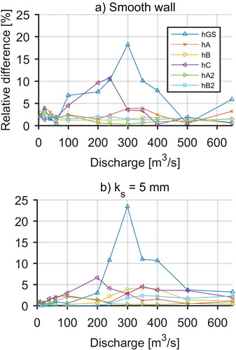
We conclude that the model is very sensitive to changes in roughness coefficient, resulting in deviations in the stage at point GS. This is mainly because the measurement point lays in a wake and is sensitive to small variations in inflow direction. The model is relatively insensitive to changes in roughness coefficient at all the other points.

Results and discussion

Water surface elevation and velocities

A key benefit of the hybrid modeling approach is the possibility to provide detailed flow fields, and the ability to easily monitor key variables in the CFD model. This is exploited to analyze the complicated flow at the field site, within the range of considered discharges (7.5–650 m³/s). Velocity magnitudes are reported for each cell, not only in selected points, and detailed water-surface elevation and surface velocity plots can be extracted from the model for the analysis. In addition, the CFD model is expanded upstream to also study the flow in the curve upstream of the measurement pool, that was not included in the physical model study.

At higher flows, the hydraulics at the site is complicated for several reasons. There is long curve ending in a rapid upstream of the measurement pool. A jet flows from the rapid into the pool. The jet increases in magnitude and changes direction with increasing discharge, causing 3-dimensional, non-uniform flow-patterns in the pool. These effects cannot be captured by a 1d- or a 2d-numerical model. The conditions are further complicated by a rock-outcrop obstruction upstream of point GS. At higher flows, the jet hits the obstruction, causing separation and recirculating flow in the wake. The critical section of the waterfall lays perpendicular to the direction of the flow through the pool, causing an approximate 90-degree bend into the waterfall, resulting in additional backwater effects upstream. There is another pool downstream of the waterfall. The difference in water level between the upper and the lower pool is approximately 5 meters at mean discharge (17 m³/s). The water level in the lower pool is controlled by a narrow section downstream, causing the lower pool to rise to the level of the bedrock weir at high discharges, and eventually causes submergence of the waterfall at very high flows.

Figure 7 shows water surface elevations and surface velocities from six different discharges. Looking at the water surface elevations, it can be observed that the upstream pool is relatively level for discharges up to 60 m³ s⁻¹. For discharges larger than 60 m³ s⁻¹, the increased momentum of inflow from the upstream rapid causes super elevation of the water surface in the outward curve, that is the left side of the pool. At Q > ∼100 m³ s⁻¹, the effects of the jet from the rapids hitting the obstruction upstream of point GS also starts to cause draw-down of the water surface on the right side of the pool. The measurement conditions at point GS becomes increasingly unstable at Q > ∼250 m³ s⁻¹, due to the conditions in the wake of the obstruction.

Figure 7. CFD model result plots for selected discharges; left: Water surface elevations; right: surface velocity.

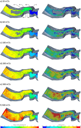
The direction of the inflow stream to the pool is to the left as it enters the pool at Q = 20 m³ s⁻¹ and smaller discharges. As the discharge increases, the main stream is pushed more to the right in the pool. Low surface velocities are observed on the left side of the river, close to point B and B2 for all considered discharges. The water surfaces spatial gradient is also small at these points, making them good candidate points for stage measurements during floods. In the curve upstream of the measurement pool the water-surface plot shows super elevation in the outer curve for all discharges larger than 60 m³ s⁻¹. The flow is split in two chutes, and the highest velocities are observed in the right-side chute as it enters the pool. From approximately 200 m³ s⁻¹ there is backwater forming where the downstream end of the curve meets the rapids upstream of the measurement pool.

High velocities at the point where the stage is measured are problematic because the stage measurement may be disturbed. If the stage is measured in a stilling well, high velocities close to the intake can cause drawdown or super elevation in the stilling well (see Herschy, 2009). For further insights in the flow characteristics, local velocities are extracted from the CFD model. Figure 8 shows velocity magnitude from the CFD model close to the bottom at the points of measurement. For example, the velocity at point GS raises to over 3 m s⁻¹ for Q > 200 m³ s⁻¹, while point B never has higher velocities than 0.5 m s⁻¹. Similarly, considering velocity magnitude, point A seems to be a better choice than point A2 with regard to stage measurement.

Figure 8. Velocity magnitudes measured close to the bottom at the measurement points.

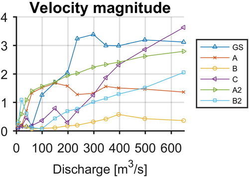
Considering the gradient of the free-surface, surface velocities, and velocities at the measurement point; point B and B2 seem to be the best locations for stage measurement during floods. Point GS, which is the current stage measurement location, has challenging conditions for the reliable measurement of stages, especially in the extrapolated range (Q > ∼250 m³ s⁻¹). The velocities past the point exceed 3 m s⁻¹ and the water surface has a sharp gradient. Point B has somewhat better conditions than point B2 regarding velocities at the point and the stability of the water surface at the point.

Synthetic stage-discharge data and rating curve

Initially, a goal of the case-study was to model the existing rating curve in point GS. However, as discussed in the validation and sensitivity chapter as well as in (Pedersen, Aberle, et al., 2018), point GS turned out to be unsuitable for modeling as well as for field measurements during large flows. The results from the scale model experiments (Pedersen, Aberle, et al., 2018) further showed that point B, on the left side of the river, was the most suitable point for stage measurements at large flows. This conclusion is also supported by the CFD modeling results, as was discussed in the previous section. As a result of the modeling effort it was therefore decided that a new flood rating curve should be constructed in point B. The resulting rating curve from the CFD model data is discussed in the further.

The stage-discharge data at point B are presented in Figure 9. The field gaugings and CFD stage-discharge data for point GS as well as the operational rating curve are also included for comparison. It can be observed that the CFD model has good agreement with the field data for discharges smaller than 200 m³ s⁻¹ at point GS. However, it should be noted that the stage at this point is quite sensitive to small spatial deviations and roughness coefficient in the upstream rapids for Q > 100 m³ s⁻¹, as was discussed in the validation and sensitivity section. Comparing the current operational rating curve to the synthetic data from the CFD model, it is also worth noting that there is a large difference for flows in the extrapolated range.

Figure 9. Current operational rating-curve for point GS and the new proposed rating-curve for point B compared to stage data from the field at point GS, and CFD data for point GS and point B.

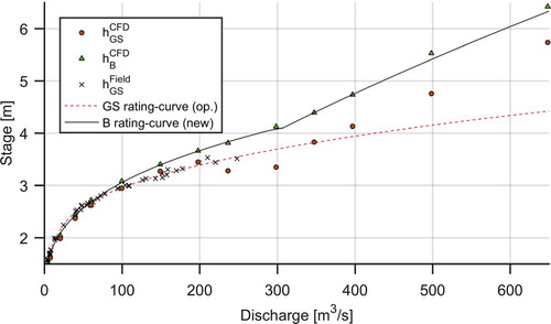
Point B is located on the opposite side of the pool from point GS (see Figure 1). From Figure 9, it can be seen that the stage at the two points (please see point h_B^CFD and h_GS^CFD in the figure) is approximately equal for Q < 100 m³ s⁻¹. For Q > 100 m³ s⁻¹, the stage at point B is higher than at point GS. This is mainly due to the obstruction and wake flow close to point GS lowering the stage at the right side of the river.

A rating curve with 2 segments was fitted to the synthetic data from the CFD model at point B (Figure 9) using the standard log–log method (WMO, 2010).

Table 1 gives the resulting parameters from equation 1(1) $Q=C(h-h_0{)}^{\wedge }b$(1) . The stage of zero flow (h₀) was fixed to 0.592. This value originates from field measurements of the stage of zero flow. The slope parameter for the first segment (b₁) is 3. This is consistent with expected values for section controls in natural rivers. For example, according to Herschy (2009) b is in practice almost always larger than 2 and often larger than 3 for section controls in deep, narrow rivers. The threshold stage between the two segments (h_s1) is 4.21 m, which corresponds to Q = 322 m³ s⁻¹. The slope of the second segment, b₂ = 1.5. This is a sharp gradient compared to the first section, and corresponds to the theoretical value for a rectangular section control or weir, but it is somewhat low for a natural section.

Table 1. Fitted multi-segment rating-curve parameters to CFD model stage-discharge data.

C1	C2	b1	b2	h01	h02	hs1
6.8	48	3	1.5	0.592	0.65	4.21

Several factors may contribute to the headloss and rise in the water level at point B, which in turn would cause a greater rating slope and lower value of b₂. The change of direction of the flow into the pool from the upstream rapids causes super-elevation at the right side of the river, and there is a head-loss and resulting backwater effect associated with the nearly 90-degree bend into the waterfall. Another suspected contributing effect is the beginning submergence of the waterfall due to the water rise in the pool downstream of the waterfall due to the contraction further downstream. However, the tailwater to headwater ratio over the waterfall expressed as (h_C – h₀₁)/(h_B2 – h₀₁) reach a maximum of 0.53 at 650 m³/s in the simulations. At these ratios the influence of the tailwater on the capacity of the waterfall can be expected to be small. For example, Tullis and Neilson (2008) report that the submergence should be >0.7 before significant reduction in capacity occurs for ogee weirs. Inspecting the simulations in detail it was observed that the backwater from the 90 degree bend propagates upstream from the water-fall and starts to influence point B at approximately300 m³/s. The main effect contributing to the change in slope of the rating is therefore likely the backwater effect due to the bend, which seem to coincide with the change of slope seen in the CFD model data (Figure 9). This will cause a change in the rating slope, and therefore also justifies the use of two rating functions with a threshold, as opposed to fitting a single rating-function.

Final remarks and conclusion

Most literature on gauging stations assumes predominantly 1-dimensional flow conditions at the site, and recommends practices based on this assumption. This is sufficient for gauging-stations located in for example wide, straight rivers or for moderate flow at location with section control. However, the case-study discussed in this paper highlights the possibilities of changes in the stage-discharge relation due to highly 3-dimensional flow, especially during flood conditions when the velocities at a site are high.

As part of a hybrid modeling approach, a CFD model was used to investigate an existing gauging station rating-curve for high flows, where no direct measurements of discharge exist. The results supported earlier scale model findings, showing that the existing curve is unreliable during high flow due to the effects of a rock-outcrop that disturbs the flow at the current measurement location. The expanded CFD model was used to produce synthetic stage-discharge data for a new rating-curve at an alternative point of measurement. Due to a spatially extended CFD model, better insight into the velocity magnitudes and detailed water-surface elevation could be obtained compared to the scale model.

This demonstrates that a validated CFD model can be a used for analyzing flow patterns at gauging stations with challenging geometry and challenging flow conditions. The CFD model in this case study generally produced results with comparable accuracy to the scale model study. The case study indicates that CFD models could be applied either as part of a hybrid modeling approach or as stand-alone modeling, given sufficient field validation data. It is important to note that neither the scale model or the CFD model required calibration of bed roughness to give the results presented. This is because the hydraulic control is exerted mainly by a critical section and is dominated by singular losses. An important limitation of the study is therefore rating curves for gauging stations with friction-dominated channel control, where the calibration of bed roughness will be necessary. Another noteworthy limitation is gauging stations with moving beds, as this case study covered a gauging station with fixed bed only.

Due to the CFD model, effects such as wake flow or effects of jets, can be studied in detail. It is emphasized that CFD models can be used to identify effects that can compromise stage measurement, such as the problems due to an obstruction or the formation of a hydraulic jump. These effects may not be readily apparent for a hydrologist observing the river at normal flow, or even at high discharges. It is further demonstrated that synthetic stage-discharge data can be produced even for locations where the conditions determining the stage is not always straight forward. This makes CFD a valuable tool for analyzing flow conditions at gauging stations at challenging locations, and for producing synthetic data for rating curves even where direct discharge measurements are not available for all flows.

Acknowledgements

The authors would like to acknowledge the Norwegian Research Council and Energy Norway for supporting this study. It is conducted within the project ES519956 ‘FlomQ – A robust framework to reduce uncertainty in flood prediction’.

Disclosure statement

No potential conflict of interest was reported by the authors.

ORCID

Øyvind Pedersen http://orcid.org/0000-0001-8166-8202

References

- Abril, J. B., & Knight, D. W. (2004). Stage-discharge prediction for rivers in flood applying a depth-averaged model. Journal of Hydraulic Research, 42(6), 616–629. doi: 10.1080/00221686.2004.9628315
- Amicarelli, A., Kocak, B., Sibilla, S., & Grabe, J. (2018). A 3D smoothed particle hydrodynamics model for erosional dam-break floods. International Journal of Computational Fluid Dynamics, 31(10), 413–434. doi: 10.1080/10618562.2017.1422731
- Bermúdez, M., Cea, L., Puertas, J., Conde, A., Martín, A., & Baztán, J. (2017). Hydraulic model study of the intake-outlet of a pumped-storage hydropower plant. Engineering Applications of Computational Fluid Mechanics, 11(1), 483–495. doi: 10.1080/19942060.2017.1314869
- CD-adapco. (2015). User guide: STAR-CCM+ Version 10.02. Melville, NY USA.
- Conway, P., O'Sullivan, J. J., & Lambert, M. F. (2013). Stage–discharge prediction in straight compound channels using 3D numerical models. Proceedings of the Institution of Civil Engineers - Water Management, 166(1), 3–15. doi: 10.1680/wama.11.00015
- Corato, G., Moramarco, T., & Tucciarelli, T. (2011). Discharge estimation combining flow routing and occasional measurements of velocity. Hydrology and Earth System Sciences, 15(9), 2979–2994. doi: 10.5194/hess-15-2979-2011
- Dargahi, B. (2006). Experimental study and 3D numerical simulations for a free-overflow spillway. Journal of Hydraulic Engineering-Asce, 132(9), 899–907. doi: 10.1061/(Asce)0733-9429(2006)132:9(899)
- Di Baldassarre, G., & Claps, P. (2011). A hydraulic study on the applicability of flood rating curves. Hydrology Research, 42(1), 10–19. doi: 10.2166/nh.2010.098
- Di Baldassarre, G., Laio, F., & Montanari, A. (2012). Effect of observation errors on the uncertainty of design floods. Physics and Chemistry of the Earth, Parts A/B/C, 42–44, 85–90. doi: 10.1016/j.pce.2011.05.001
- Di Baldassarre, G., & Montanari, A. ((2009)). Uncertainty in river discharge observations: A quantitative analysis. Hydrology and Earth System Sciences, 13(6), 913–921. doi: 10.5194/hess-13-913-2009
- Domeneghetti, A., Castellarin, A., & Brath, A. (2012). Assessing rating-curve uncertainty and its effects on hydraulic model calibration. Hydrology and Earth System Sciences, 16(4), 1191–1202. doi: 10.5194/hess-16-1191-2012
- Dymond, J. R., & Christian, R. (1982). Accuracy of discharge determined from a rating curve. Hydrological Sciences Journal-Journal Des Sciences Hydrologiques, 27(4), 493–504. doi: 10.1080/02626668209491128
- Flow-3D [Computer software]. (n.d.). Santa Fe NM, USA: Flow Science.
- Gessler, D. (2005). CFD Modeling of Spillway Performance World Water and Environmental Recources Congress 2005 (pp. 1–10). American Society of Civil Engineers.
- Hager, W. H., & Boes, R. M. (2014). Hydraulic structures: A positive outlook into the future. Journal of Hydraulic Research, 52(3), 299–310. doi: 10.1080/00221686.2014.923050
- Hargreaves, D. M., Morvan, H. P., & Wright, N. G. (2007). Validation of the volume of fluid method for free surface Calculation: The broad-crested weir. Engineering Applications of Computational Fluid Mechanics, 1(2), 136–146. doi: 10.1080/19942060.2007.11015188
- Haun, S., Olsen, N. R. B., & Feurich, R. (2011). Numerical Modeling of flow over Trapezoidal broad-crested weir. Engineering Applications of Computational Fluid Mechanics, 5(3), 397–405. doi: 10.1080/19942060.2011.11015381
- Heller, V. (2011). Scale effects in physical hydraulic engineering models. Journal of Hydraulic Research, 49(3), 293–306. doi: 10.1080/00221686.2011.578914
- Herschy, R. W. (2009). Streamflow measurement, third ed. New york, NY, USA: Taylor & Francis.
- Hirt, C. W., & Nichols, B. D. (1981). Volume of fluid (Vof) method for the dynamics of free boundaries. Journal of Computational Physics, 39(1), 201–225. doi: 10.1016/0021-9991(81)90145-5
- Kara, S., Stoesser, T., Sturm, T. W., & Mulahasan, S. (2015). Flow dynamics through a submerged bridge opening with overtopping. Journal of Hydraulic Research, 53(2), 186–195. doi: 10.1080/00221686.2014.967821
- Kirkgoz, M. S., Akoz, M. S., & Oner, A. A. (2009). Numerical modeling of flow over a chute spillway. Journal of Hydraulic Research, 47(6), 790–797. doi: 10.3826/jhr.2009.3467
- Kuczera, G. (1996). Correlated rating curve error in flood frequency inference. Water Resources Research, 32(7), 2119–2127. doi: 10.1029/96wr00804
- Lopes, P., Tabor, G., Carvalho, R. F., & Leandro, J. (2016). Explicit calculation of natural aeration using a volume-of-fluid model. Applied Mathematical Modelling, 40(17), 7504–7515. doi: 10.1016/j.apm.2016.03.033
- Moyeed, R. A., & Clarke, R. T. (2005). The use of Bayesian methods for fitting rating curves, with case studies. Advances in Water Resources, 28(8), 807–818. doi: 10.1016/j.advwatres.2005.02.005
- Novak, P., Guinot, V., Jeffrey, A., & Reeve, D. E. (2010). Hydraulic modelling – an introduction. London: Spon Press.
- Olsen, N. R. B., & Kjellesvig, H. M. (1998). Three-dimensional numerical flow modelling for estimation of spillway capacity. Journal of Hydraulic Research, 36(5), 775–784. doi: 10.1080/00221689809498602
- OpenFOAM [Computer software]. (n.d.). London: OpenFOAM Foundation.
- Pedersen, Ø., Aberle, J., & Rüther, N. (2018). Hydraulic scale modelling of the rating cuver for a gauging station with challenging geometry. Hydrology Research. ( in review).
- Pedersen, Ø, Fleit, G., Pummer, E., Tullis, B. P., & Rüther, N. (2018). Reynolds-Averaged Navier-Stokes Modeling of submerged ogee weirs. Journal of Irrigation and Drainage Engineering, 144(1), 04017059. doi: 10.1061/(asce)ir.1943-4774.0001266
- Pedersen, Ø, & Rüther, N. (2016). Hybrid modeling of a gauging station rating curve. Procedia Engineering, 154, 433–440. doi: 10.1016/j.proeng.2016.07.535
- Petersen-Øverleir, A., Soot, A., & Reitan, T. (2008). Bayesian rating curve Inference as a streamflow data Quality Assessment tool. Water Resources Management, 23(9), 1835–1842. doi: 10.1007/s11269-008-9354-5
- Rantz, S. E. (1982). Measurement and computation of streamflow. Volume, 1. Measurement of stage and discharge. Volume 2. Computation of discharge. US Geological Survey Water-Supply Paper, 2175.
- Reitan, T., & Petersen-Overleir, A. (2009). Bayesian methods for estimating multi-segment discharge rating curves. Stochastic Environmental Research and Risk Assessment, 23(5), 627–642. doi: 10.1007/s00477-008-0248-0
- Sarker, M. A., & Rhodes, D. G. (2004). Calculation of free-surface profile over a rectangular broad-crested weir. Flow Measurement and Instrumentation, 15(4), 215–219. doi: 10.1016/j.flowmeasinst.2004.02.003
- Savage, B. M., & Johnson, M. C. (2001). Flow over ogee spillway: Physical and numerical model case study. Journal of Hydraulic Engineering-Asce, 127(8), 640–649. doi:10.1061/(Asce)0733-9429(2001)127:8(640).
- Shao, Q., Dutta, D., Karim, F., & Petheram, C. (2018). A method for extending stage-discharge relationships using a hydrodynamic model and quantifying the associated uncertainty. Journal of Hydrology, 556, 154–172. doi: 10.1016/j.jhydrol.2017.11.012
- Shih, T. H., Liou, W. W., Shabbir, A., Yang, Z., & Zhu, J. (1995). A new k-ε eddy viscosity model for high reynolds number turbulent flows. Computers and Fluids, 24(3), 227–238. doi: 10.1016/0045-7930(94)00032-T
- Slotnick, J., Khodadoust, A., Alonso, J., Darmofal, D., Gropp, W., Lurie, E., & Mavriplis, D. (2014). CFD Vision 2030 Study: A Path to Revolutionary Computational Aerosciences. Hanover, MD: N.C.f.A. Information.
- STAR-CCM+ version 10.02 [Computer software]. (n.d.). Melville, NY: CD-adapco.
- Steinbakk, G. H., Thorarinsdottir, T. L., Reitan, T., Schlichting, L., Hølleland, S., & Engeland, K. (2016). Propagation of rating curve uncertainty in design flood estimation. Water Resources Research, 52(9), 6897–6915. doi: 10.1002/2015WR018516
- Toro, J. P., Bombardelli, F. A., & Paik, J. (2017). Detached eddy simulation of the nonaerated skimming flow over a stepped spillway. Journal of Hydraulic Engineering, 143(9), doi: 10.1061/(ASCE)HY.1943-7900.0001322
- Tullis, B. P., & Neilson, J. (2008). Performance of submerged ogee-crest weir head-discharge relationships. Journal of Hydraulic Engineering-Asce, 134(4), 486–491. doi: 10.1061/(Asce)0733-9429(2008)134:4(486)
- Versteeg, H. K., & Malalasekera, W. (2007). An introduction to computational fluid dynamics (2nd ed.). Upper Saddle River, USA: Pearson Education Limited.
- Wan, H., Li, R., Pu, X., Zhang, H., & Feng, J. (2018). Numerical simulation for the air entrainment of aerated flow with an improved multiphase SPH model. International Journal of Computational Fluid Dynamics, 31(10), 435–449. doi: 10.1080/10618562.2017.1420175
- WMO. (2010). Manual on Stream Gauging, WMO-No. 1044 (Vols. I and II). Geneva, Switzerland: World Meteorological Organization.
- Yang, T.-H., Ho, J.-Y., Hwang, G.-D., & Lin, G.-F. (2014). An indirect approach for discharge estimation: A combination among micro-genetic algorithm, hydraulic model, and in situ measurement. Flow Measurement and Instrumentation, 39, 46–53. doi: 10.1016/j.flowmeasinst.2014.07.003
- Zeng, J., Zhang, L., Ansar, M., Damisse, E., & González-Castro, J. (2016a). Applications of computational fluid dynamics to flow Ratings at prototype spillways and weirs. I: Data Generation and Validation. Journal of Irrigation and Drainage Engineering, 04016072. doi: 10.1061/(ASCE)IR.1943-4774.0001112
- Zeng, J., Zhang, L., Ansar, M., Damisse, E., & González-Castro, J. (2016b). Applications of computational fluid dynamics to flow Ratings at prototype spillways and weirs. II: Framework for Planning. Data Assessment, and Flow Rating. Journal of Irrigation and Drainage Engineering, 04016073. doi: 10.1061/(ASCE)IR.1943-4774.0001113