Numerical simulation of thermal pollution zones’ formations in the water environment from the activities of the power plant

ABSTRACT

In this paper, obtained numerical results of the thermal pollution from the operation of a power plant are presented when using the Irtysh River as a natural water cooling system. A two-dimensional formulation by using the “shallow water” approximation is often used as a numerical solution of such problems. For two-dimensional numerical modeling, it is possible to determine the floating flow together with its characteristics of mixing heated water discharge from lateral projections to transverse flow. Furthermore, data from the experiment and numerical values of other authors were used in order to check the conformity of the computational results. The obtained numerical values gave good agreement comparing with data from the experiment, specially the jets trajectory, the recirculation zones size and the dimensionless excess temperature distribution. The obtained data as a result of numerical simulation can be used to study problems associated with the mixing of heated water discharged from the lateral direction into the transverse flow. Also these studies were conducted to study thermal contamination under different scenarios, the impact of heated water discharge from a power plant in the Irtysh River, and the areas of thermal pollution for different velocity scenarios were determined.

KEYWORDS:

• Navier–Stokes equation
• operational capacities of the power plant
• finite volume method
• the SIMPLE algorithm
• thermal discharge
• heat exchange

Introduction

Industrial chemistry, fossil fuels and nuclear power plants use a large amount of water to cool the units and this heated water discharge returns to an environment with a higher temperature. The operation of a power plant is often associated with significant problems specific to a particular location (Abbaspour, Moghimi, & Kayhan, 2005; Hester & Doyle, 2011; Lyubimova, Lepikhin, Parshakova, Lepikhin, & Tiunov, 2018; Raptis, van Vliet, & Pfister, 2016; van Vliet et al., 2012a). Heated water prevents natural conditions in the sea, lakes or rivers that affect aquatic flora and fauna (Madden, Lewis, & Davis, 2013). In the case of thermal pollution, the heat acts as a pollutant (Ling et al., 2017; van Vliet et al., 2012b). The nuclear power plants which are located in the coastal zone usually use a large amount of water to cool the units and discharge them into the nearby water environment. Due to the fact that four to six power units can be located for each site, the huge amount of heated water could be discharged into the coastal region. The generator power is gradually increasing. Consequently most nuclear power plants are discharging heated water near the coastal region of the power plant. The location and size of the water intake and discharge systems are selected by the following criteria: (a) prevent large temperature differences between the temperatures of the reservoir and the temperatures of heated water emitted in regions with environmental vulnerabilities, in order to minimize environmental damage and (b) prevent the accumulation of heated water in the water intake area, which can significantly reduce the efficiency of the cooling system of the power plant.

In order nuclear power plant to achieve these goals, and to keep it environmentally acceptable and economically feasible and optimal, a hydrothermal analysis of the cooling water flow consumption should be carried out. This hydrothermal analysis is carried out by using mathematical models in which the continuity equation and hydrodynamic momentum equations are used to calculate the flow field and the heat transport equation for calculating the heat spread from the discharge channel from the operation of the power plant, since to do the natural experiment will be very expensive. In order to solve this technological and environmental problem, it is necessary to obtain comprehensive and reliable estimates of the temperature field parameters with respect to technological and hydrometeorological parameters (Raptis & Pfister, 2016; Wu, Buchak, Edinger, & Kolluru, 2001). To solve the harmful effects problem from the power plants on water bodies or rivers, a necessary requirement for technological and environmental constraints is obtaining detailed and complete information on the temperature fields in the discharge area under various hydrometeorological conditions.

The study of the injected heated jet into the cooled transverse flow is a very important problem, since this problem is encountered in the investigation of gas combustion chambers and drainage of sewage. In this problem, the fluid is usually injected into the transverse flow through one hole, through a holes series or through the linear holes. This problem has been investigated by many authors. In the paper (Chieh, 1987) used a simple two-dimensional model of excess temperature applied to a surface layer of constant thickness with a parallel flow for hydrothermal analysis in the Red Sea region. A more complex three-dimensional model was applied by Beckers and Van Ormelingen (1995) to conduct a thermo hydrodynamic simulation of a power plant in Zeebrugge harbour. There are also many papers that computationally simulate the behavior of heated water outfalls from the surface discharge channels.

The lateral water discharge was first numerically simulated by McGuire and Rodi (1978, 1979). In these papers, a two-dimensional mathematical model was developed. This numerical simulation was made by averaging velocity over depth and temperature propagation in open channels.

With this simulation, the side discharge in the open channel flow was analyzed and the obtained numerical values were compared with data from the experiment, which has a wide range of drainage rates for the open channel flow. Also in the paper (McGuirk & Rodi, 1979), a three-dimensional mathematical model was developed that is intended for investigating flow for the heated surface jet. The obtained numerical values were satisfactory and give greater confidence compared with data from the experiment. These results prove that using a numerical model is an effective and economical tool for researching this problem. In the paper (Park & Chung, 1983) a numerical algorithm was developed using the turbulence model with four equations, then a model was used to predict the two-dimensional vertical thermal discharge into the reservoir. In the paper (Lee, Choi, & Lee, 1994) a two-dimensional numerical model was developed for exact prediction of the temperature values, a near discharge area caused by heated water discharged into a shallow transverse flow. In the paper (Lee, Choi, & Huh, 1995) a three-dimensional numerical model was also developed. Also in this work a $k-\epsilon$ turbulent model was used to simulate thermal jet trajectory, gravitational lateral propagation and stratification.

In addition, there are many papers on three-dimensional models that examine the overall heat balance, rather than on mixing in the heated water discharge region in a nearby area. This is well described in the papers Davies, Jones, and Xing (1997) and Kim and Seo (2000), in these papers the mixing of discharged heated water was analyzed by numerical simulation. In the paper (Kim, Seo, Kang, & Oh, 2002), an analysis of the mixing process of the jet with the main channel discharging from a single immersed port using a three-dimensional hybrid mathematical model with allowance for the buoyancy forces was made, in which the simulation for the initial mixing was performed by the advection-diffusion processes and the jet integral method, were simulated using the particle tracking method.

In these works, the continuity equations, the three-dimensional Reynolds equations by using Boussinesq approximations, hydrostatic pressure, and heat transfer equations were used to simulate this process. In the paper (Lowe, Schuepfer, & Dunning, 2009), a predict of the maximum water discharge for worst-case scenarios for thermal contamination was obtained for calculating the temperature field and currents in the East River (New York), which was created under the influence of two TPPs.

Also the importance of solving spatial models for a right assessment of the thermal pollution spread in rivers is discussed in papers (Chau & Jiang, 2004; Prats, Val, Dolz, & Armengol, 2012). In the papers (Chau & Jiang, 2001; Chau & Jiang, 2002; Issakhov, 2013, 2014a) three-dimensional numerical simulations of turbulent mixing of water layers for different temperatures were carried out.

The study of the heated water emission from power plants into reservoirs or rivers and the cooling of this water have been interested in many years (Yunli, Deguan, Zhigang, & Xijun, 2006). This problem not only provides great theoretical significance for the study of the transport and thermal water movement, but also has great economic importance. Since without proper methods of heat waste management, these wastes of greater extent will cause great damage to the surrounding aquatic environment and natural flora and fauna.

For a number of significant environmental problems, successfully performed the numerical study (Gabl & Righetti, 2018; Lepikhin, Lyubimova, Parshakova, & Tiunov, 2012; Lyubimova, Lepikhin, Parshakova, & Tiunov, 2016; Lyubimova, Lepikhin, Parshakova, Konovalov, & Tiunov, 2014; Lyubimova, Lepikhin, Tsiberkin, & Parshakova, 2014; Quezada, Tamburrino, & Niño, 2018; Wu & Chau, 2006), it was confirmed that it allows quickly obtain the necessary information about the ecosystem state, which allows for effective power plants control and, in general, to prevent technological and environmental risks of the region.

The present study presents a finite difference model that uses several numbers of simplifications, but this model takes into account the river's boundaries and the heat transfer inside and across the river. This model simplification makes it possible to calculate the characteristics of the excess temperature and, at the same time, considerably shorten the calculation time. Numerical modeling was carried out for the Irtysh River, the East Kazakhstan region, the Republic of Kazakhstan with a special ecological significance, where the construction of a nuclear power plant is envisaged. And at the moment there is a very acute question about the location of the nuclear power plant, since it is necessary to optimally locate it. However, carrying out numerical simulation for the entire three-dimensional water area is very difficult from the point of view of calculation, since even the digitization of the river coastline for the three-dimensional case remains a very difficult problem. As it will need detailed satellite imagery. However, for several test problems, a two-dimensional mathematical model for the entire water body has shown very good agreement with data from the experiment, which models well the horizontal variation of the water temperature in the near and far regions from the discharge channel. The main mechanism for the formation of a temperature field around heated water discharges is its mixing or dilution with surrounding water. Therefore, for the Irtysh River, a model was used to study the temperature change in the discharge of heated water from a discharge channel into the relatively cooled water of the Irtysh River. And also in this paper the pollution areas for different temperature ranges from the plant's activity were determined. All simulations were carried out on the ANSYS Fluent.

The field of study

The project for the construction of a nuclear power plant in the Republic of Kazakhstan is currently at the stage of developing a feasibility justification. A working group has been created, which operates in close cooperation with the International Atomic Energy Agency (IAEA). The decision on the possibility of building nuclear power plants in Kazakhstan should be made before the end of 2018. And the issue of the nuclear power plant location at the moment is an important, but not the only aspect of the future operation of the power plant, which must be solved before the construction begins. Both supporters and opponents of this project implementation on the territory of the country talk more about the environmental component (environmental risks) associated with nuclear power plants. The potential location of the nuclear power plant is currently the Kurchatov city in the East Kazakhstan region, Republic of Kazakhstan, located on the left shore of the Irtysh River between Semey and Pavlodar cities, Figure 1 (The former center of the Semey nuclear test site was closed in 1991).

Figure 1. Location of the study area.

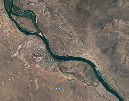
The Irtysh is a river in Asia and the longest river-inflow in the world (coordinates 61°04′50′′ N 68°49′50′′ E). It flows through the territory of The People's Republic of China, the Republic of Kazakhstan and the Russian Federation. It originates in Dzungaria on the slopes of the Mongolian Altai Black Irtysh, and then flows into Lake Zaisan, flows like Irtysh River. Moreover it is the largest tributary of the Ob River. The length of the river is 4248 km, the area of the basin is $\text{1,643,000}\text{k}{\text{m}}^{\text{2}}$. The depth of the Irtysh River ranges from 6 to 15 meters in the stream pool, up to 2–3 meters – on the whitewater. The food of the river is snow and rain. The river is calm. The speed of water flow varies from 0.5–1.5 m/s. The water temperature in the Irtysh River in the summer months is +19 to +22°C, in September it falls to +7 to +11°C, and in November the Irtysh freezes. But this phenomenon occurs only in the lower currents. The higher, the water is colder. From middle of October to middle of November, the river cramps the ice. The Irtysh River begins to be released from the ice shell from the middle of April.

One of the important parameters for limiting the water usage is the maximum water temperature in the water discharge channel area. Since a rise of even a few degrees can be detrimental to some plants and animals. Therefore, it is significant to determine the areas with the maximum temperature from the ambient temperature in the warmest season of the year (the temperature is maximally increased to 22°C). Unfortunately, the Water Code of the Republic of Kazakhstan does not limit the temperature rise on the surface of water bodies from the surrounding water temperature because of the thermal water discharge. But the Government of the Republic of Kazakhstan and the local executive bodies of the region (cities of the republican significance, the capital) in the cases of emergency situations occurrence of natural and man-made nature have the right to restrict, suspend or prohibit industrial and heat power enterprises the water usage objects and water facilities in accordance with the laws of the Republic of Kazakhstan. According to sanitary norms, the temperature of the reservoir should not increase by more than 3°C in summer and 5°C in winter.

The harmful effects of thermal pollution on aquatic ecosystems are as follows:

1. increasing the water temperature often increases the susceptibility of organisms to toxic substances (which are undoubtedly present in contaminated water);

2. the temperature may exceed the critical values for stenothermic aquatic organisms, for which even a small thermal contamination of the environment is dangerous;

3. high temperature favors replacing the usual algae flora with blue green, which promotes the water flowering;

4. when the water temperature rises, the animals need more oxygen, since in warm water its content decreases due to lower solubility;

5. as the temperature rises, the gas and chemical composition in the water changes, which leads to the growth of anaerobic bacteria and the release of poisonous gases, hydrogen sulfide and methane.

Mathematical model

Time-averaged Reynolds equations and heat transfer equation are used to simulate thermal effects on rivers or water bodies. (1) $\begin{array}{rl}\frac{\mathrm{\partial }{u}_i}{\mathrm{\partial }{x}_i}& =0\end{array}$(1) (2) $\begin{array}{rl}\frac{\mathrm{\partial }{u}_i}{\mathrm{\partial }t}+\frac{\mathrm{\partial }\left(\rho u_i{u}_j\right)}{\mathrm{\partial }{x}_j}& =\frac{\mathrm{\partial }\left(-\rho \overline{u_i^{\mathrm{\prime }}{u}_j^{\mathrm{\prime }}}\right)}{\mathrm{\partial }x}-\frac{\mathrm{\partial }P}{\mathrm{\partial }{x}_i}\\ & +\frac{\mathrm{\partial }}{\mathrm{\partial }{x}_j}\left(\mu \left(\frac{\mathrm{\partial }{u}_i}{\mathrm{\partial }{x}_j}+\frac{\mathrm{\partial }{u}_j}{\mathrm{\partial }{x}_i}\right)\right)\end{array}$(2) (3) $\begin{array}{rl}\frac{\mathrm{\partial }T}{\mathrm{\partial }t}+\frac{\mathrm{\partial }\rho u_{j}T}{\mathrm{\partial }{x}_j}& =\frac{\mathrm{\partial }\left(-\rho \overline{{u^{\mathrm{\prime }}}_j{T}^{\mathrm{\prime }}}\right)}{\mathrm{\partial }{x}_j}+\frac{\mathrm{\partial }}{\mathrm{\partial }{x}_j}\left(D\frac{\mathrm{\partial }T}{\mathrm{\partial }{x}_j}\right)\end{array}$(3) where $u_i$ – the velocity, $T$ – the temperature of the fluid,, $\rho$ – the density of the fluid, $D$ – the diffusion coefficient, $\overline{u_i^{\mathrm{\prime }}{u}_j^{\mathrm{\prime }}}$ and $\overline{u_j^{\mathrm{\prime }}{T}^{\mathrm{\prime }}}$ – averaged Reynolds velocity and turbulent heat fluxes stresses, $P$ – the fluid pressure.

The turbulent models

For the close the Reynolds-averaged Navier-Stokes Equations (1–3) different turbulent models were used:

1. the k–ε turbulence model. This is a two-parameter model that gives a general description of turbulence using two transport equations (Farhadi, Mayrhofer, Tritthart, Glas, & Habersack, 2018; Issakhov, Bulgakov, & Zhandaulet, 2019a, 2019b);

2. the k-ω turbulence model is a two-parameter general turbulence model, which is used as the closure for the Reynolds-averaged Navier-Stokes equations (Issakhov & Mashenkova, 2019);

3. The idea of the large eddy simulation method is that the velocity components are divided into the resolved and sub-grid parts. The resolved velocity is simulated by ‘large’ eddies, and the sub-grid part of the velocity is modeled by ‘small scales’. This simulation is carried out at the expense of the subgrid scale model. (Deardorff, 1970; Issakhov, 2015, 2016a, 2016b, 2017a, 2017b; Smagorinsky, 1963);

4. The idea of the DES model (Spalart, 1997) is to combine the best properties of the RANS and LES methods into one method. This method attempts to simulate the near-wall areas using the RANS method and simulate the rest of the flow using the LES method. (Issakhov, 2014b; Issakhov, Zhandaulet, & Nogaeva, 2018)

Numerical algorithm

Regions exposed to thermal effects produced by the nuclear power plant were simulated using a two-dimensional numerical model. This two-dimensional model was chosen because the horizontal change in the water temperature is practically the same as in the three-dimensional models (Chang & Chen, 1995; Chen & Hwang, 1991). In addition, it should be noticed that even the most powerful computer resources cannot provide numerical simulation for full three-dimensional cases, since large areas of a reservoir or a river do not solve this problem in a short time, because the construction of the grid will have huge dimensions. The area in which simulations were carried out using a two-dimensional model is displayed in Figure 1. The use of a two-dimensional model allows qualitatively estimate the distribution of the temperature and velocity fields in different directions. For the numerical simulation of the RANS system and the heat transfer equation, the SIMPLE (Semi-Implicit Method for Pressure-Linked Equations) algorithm was used.

The verification of the mathematical model and numerical algorithm

To test the chosen mathematical model and numerical algorithm, numerical simulations are performed on a straight open channel with a side discharge. All boundary conditions, initial conditions and dimensions of the computational domain were taken in the same way as in paper (Chang & Chen, 1995) to compare the obtained numerical values with the numerical values and with the measured values of Chen and Hwang (1991). The physical sizes of the open channel were 505 mm in length and 120 mm in width (Figure 2).

Figure 2. Geometry and boundary conditions of the test problem.

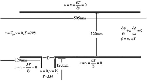
In this problem, the main channel temperature is set to 25.0°C (298 K), and the temperature of the heated water discharge from the water discharge channel was taken as 81°C (354 K). Figure 2 shows boundary conditions, initial conditions and dimensions of the computational domain of the numerical experiment for verification of the model, where the velocities were taken as $V_a=2.005\text{m/s},V_0=11.969\text{m/s}$ and the heated water discharge channel width is taken as $D=0.005\text{m}$, and the channel length is 120 mm. The total length of the main channel is 505 mm, width 120 mm (Figure 2).

The results for the temperature and velocity profiles are normalized as the different ratios according to their input conditions in accordance with $Q=\frac{T-T_a}{T_j-T_a}$ $U=\frac{\text{Velocity}U-V_a}{\text{Velocity}{U}_{max}-V_a}$where $T_a$ is the temperature of the medium, $T_j$ is the water temperature from the discharge channel, Velocity U is the velocity component along the X-axis and Velocity U_max is the maximum value of the velocity component along the X-axis.

In this paper, the numerical results with different computational grids were matched and also the obtained numerical results for different turbulent models were compared with measured values (Chen & Hwang, 1991).

Figure 3 shows the numerical results for different computational grid sizes, and it can be seen from the figure that these profiles do not differ much from each other. That is the reason for the usage of a computational grid size 189 × 45 for further simulations. Also, Figure 3 shows that the numerical values for the SST k-w and BSL k-w turbulent models are in better agreement with data from the experiment (Chen & Hwang, 1991) in comparison with the other turbulent models (Table 1). The SST k-w turbulent model showed better time spent on simulation than the BSL k-w model. So that is the reason for using the SST k-w turbulent model for all further simulations.

Figure 3. Temperature change profiles for different grid sizes and for different turbulent models.

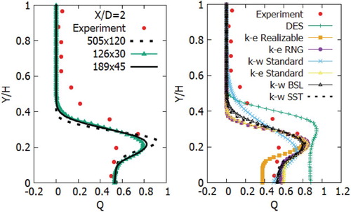
Table 1. Calculation duration and various norms of different turbulent models.

Models	Duration of calculation	$\parallel Error{\parallel }_2$
Laminar	54 min
Standard $k-\epsilon$	58 min	0.588
RNG $k-\epsilon$	59 min	0.593
Realizable $k-\epsilon$	61 min	0.579
Standard $k-\omega$	60 min	0.583
BSL $k-\omega$	58 min	0.522
SST $k-\omega$	57 min	0.510
DES SST $k-\omega$	61 min
DES Realizable $k-\epsilon$	64 min	0.755

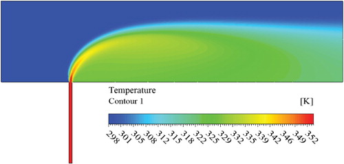
The contours of the temperature distribution behavior are shown in Figure 4. In this figure it can be noted that the trajectory of the heated water distribution from the discharge channel to the area under investigation.

Figure 4. Distribution of temperature in the open channel.

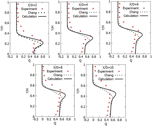
In order to complete the testing of the numerical algorithm with the test problem, numerical simulations were compared with data from the experiment (Chen & Hwang, 1991) and data from the simulations of other authors (Chang & Chen, 1995) for different cross-section profiles ($X/D=2,4,6,8,10$).

Figure 5 shows the dimensionless temperature profiles along vertical lines for different cross sections ($X/D=2,4,6,8,10$). The obtained numerical values of the simulation are satisfactory and give greater confidence compared with data from the experiment (Chen & Hwang, 1991) and the numerical results of other authors (Chang & Chen, 1995). It can be seen that the obtained numerical data from the simulations in this paper in some cross sections are even better than the numerical results of other authors (Chang & Chen, 1995). These obtained results are closer to experimental data.

Figure 5. Temperature profiles for different cross sections.

Also, an additional test problem was performed in order to check the numerical algorithm. In that case the temperature distribution is investigated from the discharge channel, located in the opposite directions at an angle of 60 degrees to the main transverse channel. With this test problem, the temperature distributions are explored by the influence of the angle between the discharge channel and the main channel. The obtained computational results were compared with the numerical values of Chang and Chen (Chang & Chen, 1995). The computational geometry and boundary conditions of this problem are presented in Figure 6.

Figure 6. Geometry and boundary conditions.

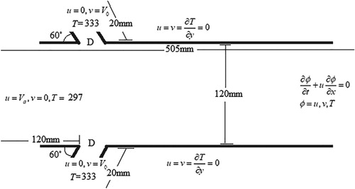
Figure 6 shows the boundary conditions for numerical simulation, where the velocities $V_a=2.37\text{m}/s,V_0=11.745\text{m/s}$ and the heated water discharge channel width $D=0.005\text{m}$, the channel length is 120 mm. The total length of the main channel is 505 mm, the width is 120 mm (Figure 6).

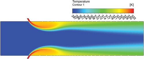
So, Figure 7 shows the temperature distribution contours for the oppositely directed transverse flows at an angle of ${60}^{\circ }$, where the symmetrical trajectory of the distribution of heated water from the water discharge channels in the simulated area can be observed.

Figure 7. Contours of temperature propagation for oppositely directed transverse flows at an angle of ${60}^{\circ }$.

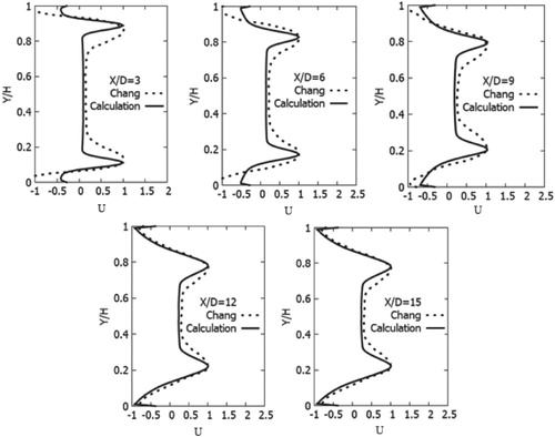
The horizontal flow velocity profiles for different cross sections ($X/D=3,6,9,12,15$) illustrated in Figure 8. From the numerical results, it can be noticed that these results have good matching with the results of other authors (Chang & Chen, 1995). The results show that the horizontal velocity component has a maximum value near the lateral walls of the main transverse channel, but towards the middle of the channel the velocity decreases, regardless of the cross section. Also from the results it can be concluded that at a distance from the discharge channel the maximum speed is moved from the side walls to the middle of the channel.

Figure 8. Horizontal velocity profiles for different sections ($X/D=3,6,9,12,15$).

Numerical results for various angles of the transverse discharge channel

In this section flows in a channel with a transverse discharge are modeled analogically to the previous section. But the difference is the effect of changing the angle of the transverse channel on the temperature propagation that is also considered here (Figure 9). The boundary conditions and dimensions of the computational domain associated with the implementation of these calculations are the same as the boundary conditions that were noted in Figure 2 (except for the angle). The angles between the main transverse channels and the discharge channel varied between ${30}^{\circ }-{150}^{\circ }$. Below the constructions of temperature profiles and horizontal velocity components at different vertical cross sections could be found. Figures 10–19 show dimensionless temperature profiles and horizontal velocity components for different vertical cross sections ($X/D=2,4,6,8,10$) at different angles (${30}^{\circ }-{150}^{\circ }$) of the transverse channel. It can be observed from Figures 10–14 that the angle of the transverse channel is changed, the results vary greatly. So from the results it can be seen that at an angle of ${30}^{\circ }$ the temperature reaches a maximum value, however, this current does not detach from the side wall of the main channel. Also, it can also be noted that as the angle of the water discharge channel increases, the temperature drops and the lowest temperature is observed at an angle of ${150}^{\circ }$. This scene remains practically unchanged independently of the distance from the water discharge channel. It can be concluded that when the angle of the discharge is reduced, although the propagation area is minimal, the maximum temperature is reached. And with an increase in the angle of the discharge channel the maximum temperature is lower, but the contamination area is large, the pollution area for the angle of ${150}^{\circ }$ is practical 5 times greater than in area at ${30}^{\circ }$.

Figure 9. Geometry and boundary conditions.

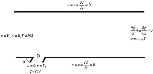
Figure 10. Dimensionless temperature profiles for the vertical cross section $X/D=2$ at different angles (${30}^{\circ }-{150}^{\circ }$) of the transverse channel.

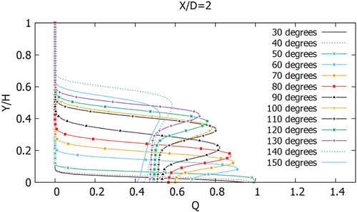
Figure 11. Dimensionless temperature profiles for the vertical cross section $X/D=4$ at different angles (${30}^{\circ }-{150}^{\circ }$) of the transverse channel.

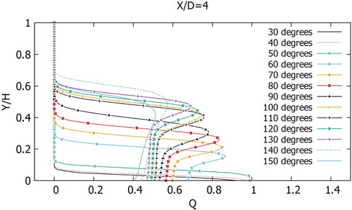
Figure 12. Dimensionless temperature profiles for the vertical cross section $X/D=6$ at different angles (${30}^{\circ }-{150}^{\circ }$) of the transverse channel.

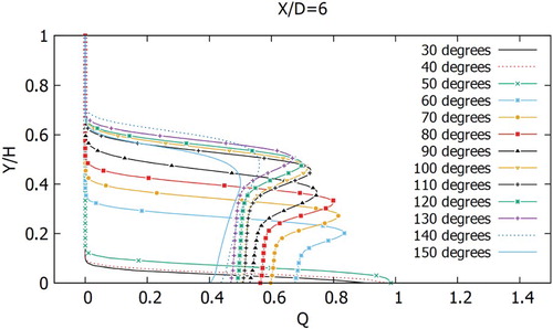
Figure 13. Dimensionless temperature profiles for the vertical cross section $X/D=8$ at different angles (${30}^{\circ }-{150}^{\circ }$) of the transverse channel.

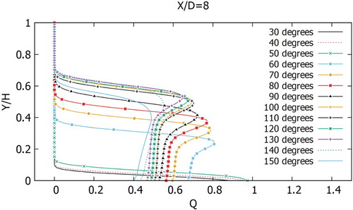
Figure 14. Dimensionless temperature profiles for the vertical cross section $X/D=10$ at different angles (${30}^{\circ }-{150}^{\circ }$) of the transverse channel.

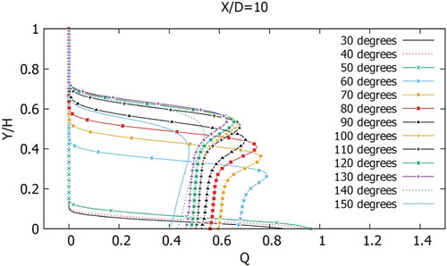
Figure 15. Dimensionless horizontal velocity component profiles for the vertical cross section $X/D=2$ at different angles (${30}^{\circ }-{150}^{\circ }$) of the transverse channel.

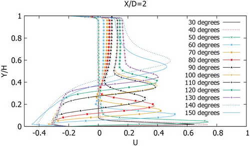
Figure 16. Dimensionless horizontal velocity component profiles for the vertical cross section $X/D=4$ at different angles (${30}^{\circ }-{150}^{\circ }$) of the transverse channel.

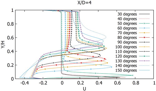
Figure 17. Dimensionless horizontal velocity component profiles for the vertical cross section $X/D=6$ at different angles (${30}^{\circ }-{150}^{\circ }$) of the transverse channel.

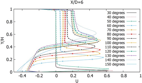
Figure 18. Dimensionless horizontal velocity component profiles for the vertical cross section $X/D=8$ at different angles (${30}^{\circ }-{150}^{\circ }$) of the transverse channel.

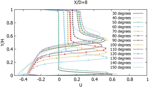
Figure 19. Dimensionless horizontal velocity component profiles for the vertical cross section $X/D=10$ at different angles (${30}^{\circ }-{150}^{\circ }$) of the transverse channel.

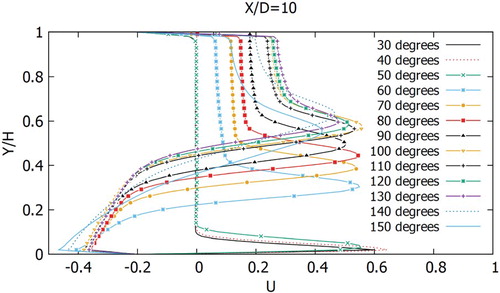
The horizontal velocity components for different vertical cross sections ($X/D=2,4,6,8,10$) at different angles (${30}^{\circ }-{150}^{\circ }$) of the transverse channel are illustrated on the Figures 15–19. From these figures, it is evident that the increase of the transverse discharge channel’s angle causes a reverse flow. So this consequently leads to an increase in the area of temperature contamination. As for temperature profiles, this character remains practically unchanged for different cross sections from the water discharge channel. It will be possible to draw the appropriate conclusions that when the water discharge channel angle of the flow is reduced, the flow is rectilinear and practical, no reverse flows are formed, and this character can be noticed for angles (${30}^{\circ }-{150}^{\circ }$). So with the increase in the water discharge channel angle, a reverse flow forms and eventually becomes larger and the maximum reverse flow is observed at a large angle of the water discharge channel.

Numerical results of thermal pollution zones’ formations on the Irtysh River

The possible but not exact location of the nuclear power plant construction at the moment is the Kurchatov city in the East Kazakhstan region, Republic of Kazakhstan. That is located on the left shore of the Irtysh River between the cities of Semey and Pavlodar. Because of that, this work will evaluate the temperature distribution from the location of the nuclear power plant. Moreover different water discharge rates will be considered. For these purposes, several important criteria are pursued in order to locate the NPPs in a given locality. Due to the fact that there is no bridge near the Kurchatov city between the left and right shores, the location of the nuclear power plant is preferable to be located on the left shore of the Irtysh River, as it is the populated locality. And to ensure that future employees of the power plant do not spend extra time for travel. And also the location of the nuclear power plant on the left shore makes it possible not to build a bridge that is economically very profitable.

The estimated computational area is 31 km by 31 km, satellite snapshot can be seen in Figure 1, and the calculation area is shown in Figure 20, the distance between the city and the NPP is taken about 5 km.

Figure 20. Calculation area.

In this problem, the flow speed of the Irtysh River was taken as an average speed of the river flow 1.5 m/s, and for the heated water discharge rate from the water discharge channel, three scenarios were taken: 2 m/s (scenario 1), 4 m/s (scenario 2) and 8 m/s (scenario 3), the velocities for all scenarios were directed by the Y-axis. During the simulation, the water temperature of the Irtysh River was taken as + 22°C, and the temperature of the heated water that was discharged from the water discharge channel of the nuclear power plant was taken as + 35°C. All the details of the scenarios are reflected in Table 2.

Table 2. Parameters used in the main scenarios.

Scenarios	Ejection rate	Ejection temperature	Ejection volume	River speed	River temperature
1	2 m/s	+35°	2 m^3/s	1.5 m/s	+22°
2	4 m/s	+35°	4 m^3/s	1.5 m/s	+22°
3	8 m/s	+35°	8 m^3/s	1.5 m/s	+22°

Two types of computational grids were used for numerical simulation:

1. computational grid, which has tetragonal elements with a grid size of 5 m, which were uniformly distributed over the whole computational domain of the river and the computational grid was clustered to the water discharge channel area and the element size of this region was 0.2 m;

2. computational grid, similar to the first one but the computational grid was clustered to the water discharge channel area and the element size of this region was 0.1 m;

Figure 21 shows the numerical results for different computational grid sizes. Also it can be seen that these temperature profiles do not differ much from each other for different computational grids. And in further simulations the computational grid with the element size of this region 0.2 m will be used. Since this computational grid has optimal parameters, such as minimum CPU execution time and accuracy of the calculation.

Figure 21. Temperature profiles on the first line for different computational meshes.

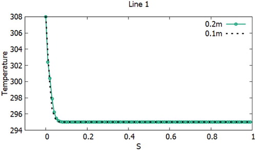
The computational grid consisted of 646142 tetragonal elements with a dimension of 5 m for one cell, which was uniformly distributed over the entire area of the river. Furthermore a computational grid was clustered to the water discharge channel area and the element size of this region was 0.2 m, this clustering was done in order to obtain the best numerical results.

Figures 22–27 show the contours of temperature distribution on the Irtysh River for all three scenarios (the heated water discharge rate from the water discharge channel: 2, 4, 8 m/s). In these figures, the temperature distribution along the river is reflected in different scales. From these results, it is obvious that with increasing discharge rates from the water discharge channel, the contaminated water area also increases. And at low rates the heated water distribution along the river occurs along the shore (Figures 22 and 23).

Figure 22. Distribution of heated water at discharge rate 2 m/s from the water discharge channel (scenario 1).

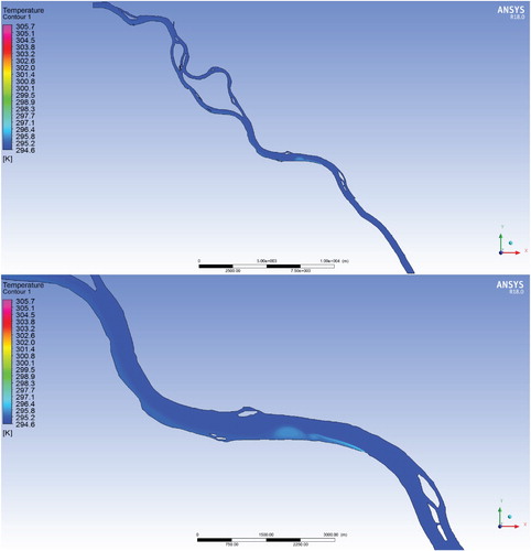
Figure 23. Distribution of heated water at discharge rate 2 m/s from the water discharge channel (scenario 1).

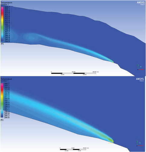
Figure 24. Distribution of heated water at discharge rate 4 m/s from the water discharge channel (scenario 2).

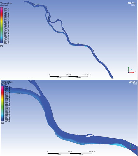
Figure 25. Distribution of heated water at discharge rate 4 m/s from the water discharge channel (scenario 2).

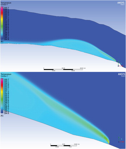
Figure 26. Distribution of heated water at discharge rate 8 m/s from the water discharge channel (scenario 3).

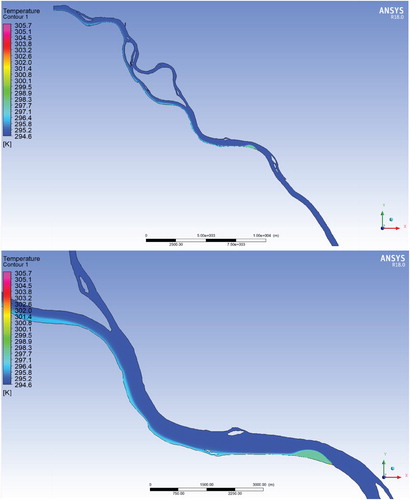
Figure 27. Distribution of heated water at discharge rate 8 m/s from the water discharge channel (scenario 3).

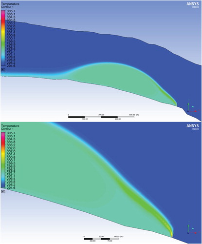
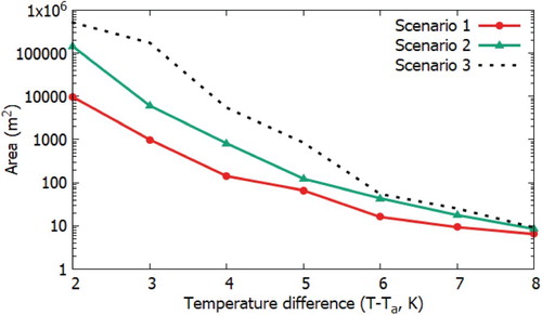
The purpose of this calculation is to assess the extent of the heated water distribution from the nuclear power plants operating at different heated water discharge rates from the water discharge channel. The conditions associated with the implementation of these scenarios are the most unfavorable from the point of view by using the ecological safety of the aquatic environment. All parameters for numerical study of these scenarios are given in Table 2. The estimated time for all scenarios is taken as 10 days (240 h). Area of heated water zones on the river (${\text{m}}^2$), where discharged the heated water temperature exceeds the ambient temperature of the aquatic environment is shown in Figure 28. Even more the consideration was done for all the three scenarios. As it can be seen from this figure, the area of the heated water zone, where the temperature increase from the river water temperature by 3°C, was about for three scenarios: $1000,6100,175,000{\text{m}}^2$, respectively. However, it can also be noted from the figure that the temperature difference of 8°C, heated water areas for all three scenarios are approximately the same ($6.45,8.5,9.12{\text{m}}^2$). The largest temperature contamination area can be observed at a temperature difference from the ambient temperature of 1°C and at the maximum heated water discharge rate (scenario 3). However, the heated water area at a temperature difference of 3°C is also very large, so at 1 m/s the contamination area is $1000{\text{m}}^2$, and at 8 m/s the contamination area is already $175,000{\text{m}}^2$, which is 175 times greater than at a speed 1 m/s.

Figure 28. Area of heated water zones on the river (${\text{m}}^2$), where discharged the heated water temperature exceeds the ambient temperature of the aquatic environment.

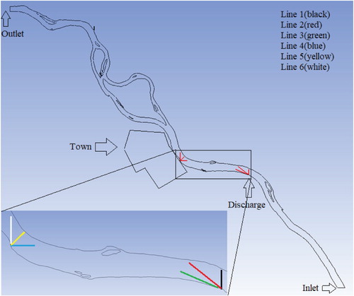
Below in Figures 29–34, the temperature profiles are plotted on different lines, the locations and directions of these lines are shown in Figure 20. Two points were used to measure the temperature distribution and three lines were located at each point (Figure 20). One point was located on the water discharge channel, and the other was a little far away from the water discharge channel, near the Kurchatov city. From these results, it can be clear that the area of heated water is much higher at a speed of 8 m/s. While in Figure 29 – the distribution of heated water at low speeds occurs near the shores along the Irtysh River. The temperature distribution along the river from the water discharge channel takes place along the heated water trajectory, which detached from the water discharge channel (shore) and tends to the middle of the Irtysh River for high speeds. This flow nature is due to the fact that the speed of the Irtysh River is 1.5 m/s, which is not quite enough to affect the heated water trajectory that has been discharged from the water discharge channel. However, it is evident that the further the heated water from the water discharge channel is located, the trajectory of the heated water approaches the Irtysh River, this is due to the fact that the influence of the speed of the discharge channel is already lost and remote heated waters are more susceptible to changes in the course of the river (Table 3).

Figure 29. Temperature profiles on the first line for three scenarios.

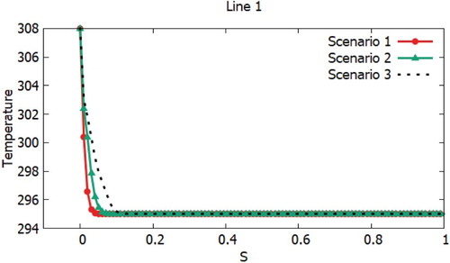
Figure 30. Temperature profiles on the second line for three scenarios.

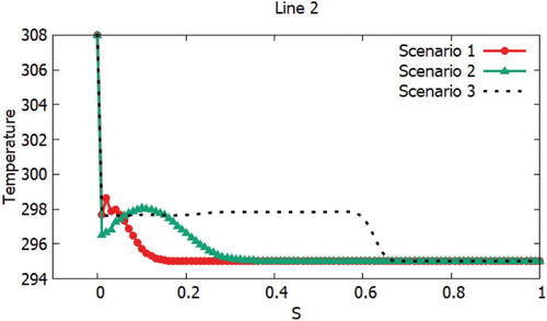
Figure 31. Temperature profiles on the third line for three scenarios.

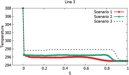
Figure 32. Temperature profiles on the fourth line for three scenarios.

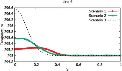
Figure 33. Temperature profiles on the fifth line for three scenarios.

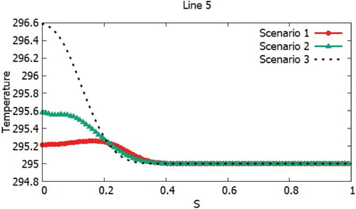
Figure 34. Temperature profiles on the sixth line for three scenarios.

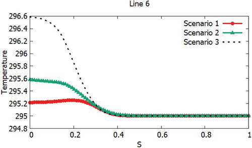
Table 3. Area of thermal pollution zones (${\text{m}}^2$) on the river at different temperature ranges for three scenarios.

	Temperature ranges
Scenarios	296–297 K	297–298 K	298–299 K	299–300 K	300–301 K	301–302 K	302–303 K
1	9663.44	999.33	142.2	66.44	16.1	9.32	6.45
2	142,790	6099.14	819	123.84	43.69	17.8	8.5
3	516,670	174,630	5471.71	851.87	54.89	25.35	9.12

Conclusions

Today, the use of reservoirs or rivers to cool heated water from the activities of the large TPP and NPP are the most extensive types of systems. The formulated problem was solved numerically by analyzing the ecological situation in the region for various heated water discharge rates from the water discharge channel into the Irtysh River, in the vicinity of the Kurchatov city at the potential location for the construction of the nuclear power plant. To solve the problem, two test problems were simulated numerically. In both cases, the obtained numerical solutions were compared with data of other authors (Chang & Chen, 1995) from the numerical simulation. Moreover the first case additionally was compared with experimental data (Chen & Hwang, 1991). And also the temperature distribution in the channel with a cross discharge with different angles of the transverse channel (${30}^{\circ }-{150}^{\circ }$) was additionally simulated.

Based on the proven mathematical model and numerical algorithm, temperature distribution simulations were carried out for the heated water discharge into the Irtysh River at different velocities from the water discharge channel. From the obtained numerical results, it can be observed that the temperature distribution on the left shore of the Irtysh River, where the heated water discharge channel is located, significantly increases downstream of the river to the city of Kurchatov. It was also found that the area with the difference in the water temperature emitted from the river water temperature exceeding the maximum possible value in the summertime by 3°C is quite large. So the area of thermal pollution accustoming to 3°C at a discharge speed of 1 m/s is $1000{\text{m}}^2$, and at a speed of 8 m/s the area was $175,000{\text{m}}^2$, which is 175 times higher compared to a speed of 1 m/s; these temperature changes may exceed the critical value for aquatic organisms and plants, for which even a small temperature change is dangerous.

Future studies in this field should continue to examine in describing the distribution of heated water discharge to the aquatic medium. With the obtained numerical data it will be possible to determine in advance the optimal location of TPPs and NPPs relative to settlements. Moreover it will help to minimize the damage from emissions for people, flora and fauna.

It should be noted that for this study there are many limitations. The first limitation is the computational grid size, since even the most powerful computational clusters cannot provide data from the numerical simulation for full three-dimensional cases, because of large areas of the reservoir or river. This is not a short time problem, because of the huge dimensions of the constructed computational grid. The second limitation is the complexity of the implementation and analysis of experimental research in the distribution of discarded heat water into the river from the activities of thermal and nuclear power plants.

Disclosure statement

No potential conflict of interest was reported by the authors.

Additional information

Funding

This work is supported by the grant from the Ministry of Education and Science of the Republic of Kazakhstan.

References

- Abbaspour, A. H. J., Moghimi, P., & Kayhan, K. (2005). Modeling of thermal pollution in coastal area and its economical and environmental assessment. International Journal of Environmental Science & Technology, 2(1), 13–26. doi: 10.1007/BF03325853
- Beckers, J.-M., & Van Ormelingen, J.-J. (1995). Thermohydrodynamical modelling of a power plant in the Zeebrugge Harbour. Journal of Hydraulic Research, 33(2), 163–180. doi: 10.1080/00221689509498668
- Chang, Y. R., & Chen, K. S. (1995). Prediction of opposing turbulent line jets discharged laterally into a confined crossflow. International Journal of Heat and Mass Transfer, 38(9), 1693–1703. doi: 10.1016/0017-9310(94)00277-3
- Chau, K. W., & Jiang, Y. W. (2001). 3D numerical model for Pearl River estuary. Journal of Hydraulic Engineering, 127(1), 72–82. doi: 10.1061/(ASCE)0733-9429(2001)127:1(72)
- Chau, K. W., & Jiang, Y. W. (2002). Three-dimensional pollutant transport model for the Pearl River estuary. Water Research, 36(8), 2029–2039. doi: 10.1016/S0043-1354(01)00400-6
- Chau, K. W., & Jiang, Y. W. (2004). A three-dimensional pollutant transport model in orthogonal curvilinear and sigma coordinate system for Pearl River estuary. International Journal of Environment and Pollution, 21(2), 188–198. doi: 10.1504/IJEP.2004.004185
- Chen, K. S., & Hwang, J. Y. (1991). Experimental study on the mixing of one- and dual-line heated jets with a cold crossflow in a confined channel. AIAA Journal, 29, 353–360. doi: 10.2514/3.10586
- Chieh, S.-H. (1987). Two dimensional numerical model of thermal discharges in coastal regions. Journal of Hydraulic Engineering, 113(8), 1032–1040. doi: 10.1061/(ASCE)0733-9429(1987)113:8(1032)
- Davies, A. M., Jones, J. E., & Xing, J. (1997). Review of recent development in tidal hydrodynamic modeling. I: Spectral models, II: Turbulence energy models. Journal of Hydraulic Engineering, 123(4), 278–302. doi: 10.1061/(ASCE)0733-9429(1997)123:4(278)
- Deardorff, J. (1970). A numerical study of three-dimensional turbulent channel flow at large Reynolds numbers. Journal of Fluid Mechanics, 41(2), 453–480. doi: 10.1017/S0022112070000691
- Farhadi, A., Mayrhofer, A., Tritthart, M., Glas, M., & Habersack, H. (2018). Accuracy and comparison of standard k-ϵ with two variants of k-ω turbulence models in fluvial applications. Engineering Applications of Computational Fluid Mechanics, 12(1), 216–235. doi: 10.1080/19942060.2017.1393006
- Gabl, R., & Righetti, M. (2018). Design criteria for a type of asymmetric orifice in a surge tank using CFD. Engineering Applications of Computational Fluid Mechanics, 12(1), 397–410. doi: 10.1080/19942060.2018.1443837
- Hester, E. T., & Doyle, M. W. (2011). Human impacts to river temperature and their effects on biological processes: A quantitative synthesis. JAWRA Journal of the American Water Resources Association, 47, 571–587. doi: 10.1111/j.1752-1688.2011.00525.x
- Issakhov, A. (2013). Mathematical modeling of the influence of thermal power plant on the aquatic environment with different meteorological condition by using parallel technologies. Power, Control and Optimization, 239, 165–179. doi: 10.1007/978-3-319-00206-4_11
- Issakhov, A. (2014a). Mathematical modeling of thermal process to aquatic environment with different hydro meteorological conditions. The Scientific World Journal, 2014, 678095. doi: 10.1155/2014/678095
- Issakhov, A. (2014b). Modeling of Synthetic turbulence Generation in boundary layer by using Zonal RANS/LES method. International Journal of Nonlinear Sciences and Numerical Simulation, 15(2), 115–120. doi: 10.1515/ijnsns-2012-0029
- Issakhov, A. (2015). Mathematical modeling of the discharged heat water effect on the aquatic environment from thermal power plant. International Journal of Nonlinear Science and Numerical Simulation, 16(5), 229–238. doi: 10.1515/ijnsns-2015-0047
- Issakhov, A. (2016a). Mathematical modeling of the discharged heat water effect on the aquatic environment from thermal power plant under various operational capacities. Applied Mathematical Modelling, 40(2), 1082–1096. doi: 10.1016/j.apm.2015.06.024
- Issakhov, A. (2016b). Numerical modelling of distribution the discharged heat water from thermal power plant on the aquatic environment. AIP Conference Proceedings, 1738, 480025.
- Issakhov, A. (2017a). Numerical study of the discharged heat water effect on the aquatic environment from thermal power plant by using two water discharged pipes. International Journal of Nonlinear Sciences and Numerical Simulation, 18(6), 469–483. doi: 10.1515/ijnsns-2016-0011
- Issakhov, A. (2017b). Numerical modelling of the thermal effects on the aquatic environment from the thermal power plant by using two water discharge pipes. AIP Conference Proceedings, 1863, 560050.
- Issakhov, A., Bulgakov, R., & Zhandaulet, Y. (2019a). Numerical simulation of the dynamics of particle motion with different sizes. Engineering Applications of Computational Fluid Mechanics, 13(1), 1–25. doi: 10.1080/19942060.2018.1545253
- Issakhov, A., Bulgakov, R., & Zhandaulet, Y. (2019b). Numerical study of the Dynamics of Particles Motion with different sizes from Coal-Based thermal power plant. International Journal of Nonlinear Sciences and Numerical Simulation. doi: 10.1515/ijnsns-2018-0182
- Issakhov, A., & Mashenkova, A. (2019). Numerical study for the assessment of pollutant dispersion from a thermal power plant under the different temperature regimes. International Journal of Environmental Science and Technology. doi: 10.1007/s13762-019-02211-y
- Issakhov, A., Zhandaulet, Y., & Nogaeva, A. (2018). Numerical simulation of dam break flow for various forms of the obstacle by VOF method. International Journal of Multiphase Flow, 109, 191–206. doi: 10.1016/j.ijmultiphaseflow.2018.08.003
- Kim, D. G., & Seo, I. W. (2000). Modeling the mixing of heated water discharged from a submerged multiport diffuser. Journal of Hydraulic Research, 38(4), 259–270. doi: 10.1080/00221680009498325
- Kim, Y. D., Seo, I. W., Kang, S. W., & Oh, B. C. (2002). Jet integral-particle tracking hybrid model for single buoyant jets. Journal of Hydraulic Engineering, 128(8), 753–760. doi: 10.1061/(ASCE)0733-9429(2002)128:8(753)
- Lee, N. J., Choi, H. S., & Huh, J. Y. (1995). A three-dimensional turbulence model for the thermal discharge into cross flow field. Journal of Korean Society of Coastal and Ocean Engineers, 7(2), 148–155.
- Lee, N. J., Choi, H. S., & Lee, K. S. (1994). A comparative study of two-dimensional numerical models for surface discharge of heated water into cross flow field. Journal of Korean Society of Coastal and Ocean Engineers, 6(1), 40–50.
- Lepikhin, A. P., Lyubimova, T. P., Parshakova, Y. N., & Tiunov, A. A. (2012). Discharge of excess brine into water bodies at potash industry works. Journal of Mining Science, 48(2), 390–397. doi: 10.1134/S1062739148020220
- Ling, F., Foody, G. M., Du, H., Ban, X., Li, X., Zhang, Y., & Du, Y. (2017). Monitoring thermal pollution in rivers downstream of dams with Landsat ETM+ thermal infrared images. Remote Sensing, 9(11), 1175. doi: 10.3390/rs9111175
- Lowe, S. A., Schuepfer, F., & Dunning, D. J. (2009). Case study: Three-dimensional hydrodynamic model of a power plant thermal discharge. Journal of Hydraulic Engineering, 135(4), 247–256. doi: 10.1061/(ASCE)0733-9429(2009)135:4(247)
- Lyubimova, T., Lepikhin, A., Parshakova, Y., Konovalov, V., & Tiunov, A. (2014). Formation of the density currents in the zone of confluence of two rivers. Journal of Hydrology, 508, 328–342. doi: 10.1016/j.jhydrol.2013.10.041
- Lyubimova, T., Lepikhin, A., Parshakova, Y., Lepikhin, Y., & Tiunov, A. (2018). The modeling of the formation of technogenic thermal pollution zones in large reservoirs. International Journal of Heat and Mass Transfer, 126, 342–352. doi: 10.1016/j.ijheatmasstransfer.2018.05.017
- Lyubimova, T., Lepikhin, A., Parshakova, Y., & Tiunov, A. (2016). The risk of river pollution due to washout from contaminated floodplain water bodies during periods of high magnitude floods. Journal of Hydrology, 534, 579–589. doi: 10.1016/j.jhydrol.2016.01.030
- Lyubimova, T., Lepikhin, A., Tsiberkin, K., & Parshakova, Y. (2014). Self-oscillations in large storages of highly mineralized brines. Journal of Geophysical Research, 16, EGU2014-10785.
- Madden, N., Lewis, A., & Davis, M. (2013). Thermal effluent from the power sector: An analysis of once-through cooling system impacts on surface water temperature. Environmental Research Letters, 8, 035006. doi: 10.1088/1748-9326/8/3/035006
- McGuirk, J. J., & Rodi, W. (1978). A depth-averaged mathematical model for the near field of the side discharge into open-channel flow. Journal of Fluid Mechanics, 86(4), 761–781. doi: 10.1017/S002211207800138X
- McGuirk, J. J., & Rodi, W. (1979). Mathematical modeling of three-dimensional heated surface jets. Journal of Fluid Mechanics, 95(4), 609–633. doi: 10.1017/S0022112079001610
- Park, S. W., & Chung, M. K. (1983). Prediction of 2-dimensional unsteady thermal discharge into a reservoir. J Korean Soc Mech Eng, 7(4), 451–460.
- Prats, J., Val, R., Dolz, J., & Armengol, J. (2012). Water temperature modeling in the lower Ebro River (Spain): heat fluxes, equilibrium temperature, and magnitude of alteration caused by reservoirs and thermal effluent. Water Resources Research, 48, W05523. doi: 10.1029/2011WR010379
- Quezada, M., Tamburrino, A., & Niño, Y. (2018). Numerical simulation of scour around circular piles due to unsteady currents and oscillatory flows. Engineering Applications of Computational Fluid Mechanics, 12(1), 354–374. doi: 10.1080/19942060.2018.1438924
- Raptis, C. E., & Pfister, S. (2016). Global freshwater thermal emissions from steam-electric power plants with once-through cooling systems. Energy, 97, 46–57. doi: 10.1016/j.energy.2015.12.107
- Raptis, C. E., van Vliet, M. T. H., & Pfister, S. (2016). Global thermal pollution of rivers from thermoelectric power plants. Environmental Research Letters, 11(10), 104011. doi: 10.1088/1748-9326/11/10/104011
- Smagorinsky, J. (1963). General Circulation Experiments with the Primitive equations. Monthly Weather Review, 91(3), 99–164. doi: 10.1175/1520-0493(1963)091<0099:GCEWTP>2.3.CO;2
- Spalart, P. R. (1997). Comments on the feasibility of LES for wing and on a hybrid RANS/LES approach. 1st ASOSR Conference on DNS/LES, Arlington, TX.
- van Vliet, M. T. H., Yearsley, J. R., Franssen, W. H. P., Ludwig, F., Haddeland, I., Lettenmaier, D. P., & Kabat, P. (2012a). Coupled daily streamflow and water temperature modeling in large river basins. Hydrology and Earth System Sciences, 16, 4303–4321. doi: 10.5194/hess-16-4303-2012
- van Vliet, M. T. H., Yearsley, J. R., Ludwig, F., Vögele, S., Lettenmaier, D. P., & Kabat, P. (2012b). Vulnerability of US and European electricity supply to climate change. Nature Climate Change, 2, 676–681. doi: 10.1038/nclimate1546
- Wu, C. L., & Chau, K. W. (2006). Mathematical model of water quality rehabilitation with rainwater utilization – a case study at Haigang. International Journal of Environment and Pollution, 28(3–4), 534–545. doi: 10.1504/IJEP.2006.011227
- Wu, J., Buchak, E. M., Edinger, J. E., & Kolluru, V. S. (2001). Simulation of cooling-water discharges from power plants. Journal of Environmental Economics and Management, 61, 77–92.
- Yunli, Y., Deguan, W., Zhigang, W., & Xijun, L. (2006). Numerical simulation of thermal discharge based on FVM method. Journal of Ocean University of China, 5(1), 7–11. doi: 10.1007/BF02919366