Towards experimental and modeling study of heat transfer performance of water- SiO₂ nanofluid in quadrangular cross-section channels

ABSTRACT

Nanofluids have found extended applications in different industrial and engineering systems nowadays. This study aims to investigate the accurate prediction of SiO₂ nanofluid effect on the heat transfer performance, specifically convective heat transfer coefficient (H), of a quadrangular cross-section channel by considering affecting fluid flow specifications factors of Re, Pr, and concentration of nanoparticles (x) in the employing working fluid. An experimental setup is used to prepare a database consisting of 270 data points on the H, of SiO₂ nanofluids. These data are then applied to develop predictive models based on three intelligent algorithms, namely multi-layer perceptron (MLP), adaptive neuro-fuzzy inference system (ANFIS), and least squares support vector machine (LSSVM), respectively. Graphical and statistical error criterions are carried out to evaluate the credibility of the proposed approaches. The LSSVM method had the precise performance regarding the mean squared error (MSE) and the coefficient of determination (R²) of 59.7 and 0.9992, respectively. A sensitivity analysis is also carried out to assess the impact of different parameters on the H demonstrating that the Prandtl number has the highest impact with a relevancy factor (r) of 0.524.

KEYWORDS:

• Convective heat transfer coefficient
• cross-section channels
• nanofluid
• intelligent approaches
• optimization

Nomenclature

Abbreviations

AI	=	Artificial Intelligence
ANFIS	=	Adaptive neuro fuzzy inference system
ANN	=	Artificial neural network
ARD	=	Average relative deviation
FIS	=	Fuzzy inference system
LSSVM	=	Least squares support vector machine
MF	=	Membership function
MLP-ANN	=	Multilayer perceptron artificial neural network
MSE	=	Mean squared error
PSO	=	Particle swarm optimization
RBF	=	Radial basis function
RMSE	=	Root mean squared error
STD	=	Standard deviation
SVM	=	Support vector machine

Symbols

ak	=	Lagrangian multipliers
b	=	Bias term
c	=	Tuning parameter of LSSVM
Dmax	=	Maximum value of a variable
Dmin	=	Minimum value of a variable
Dn	=	Normalized value of a variable
E	=	Error function
ek	=	Error variable in LSSVM
H	=	Hat matrix
H*	=	Warning leverage
Hcal.	=	Calculated heat transfer coefficient
Hexp.	=	Experimental heat transfer coefficient
${\overline{H}}^{\exp }$	=	Average experimental heat transfer coefficient
M	=	Overall output parameter of the MLP-ANN
mi	=	Linear parameters in ANFIS
Nc	=	Number of clusters in ANFIS
ni	=	Linear parameters in ANFIS
NMF	=	Number of membership function’s parameters
Nv	=	Number of variables in ANFIS
O	=	Layer’s output in ANFIS
Pr	=	Prandtl number
R2	=	Coefficient of determination
Re	=	Reynolds number
ri	=	Linear parameters in ANFIS
W	=	Firing strength parameter in ANFIS
Wi	=	Weight vector for neurons in hidden layer of the MLP-ANN
Wi,3	=	Weight vector for neurons in output layer of the MLP-ANN
wT	=	Transposed output layer vector
$\overline{w}$	=	Normalized Firing strength
X	=	Input parameter in ANFIS
X	=	Nanofluid’s mass concentration
xk	=	Input of the kth data
Xk,i	=	ith input value
${\overline{X}}_k$	=	Average value of the kth input parameter
Yi	=	ith output value
yk	=	Output of the kth data
$\overline{y}$	=	Average value of the output parameter
Z	=	Gaussian center

Greek Letters

γ	=	regulation parameter
ε	=	Function approximations’ precision
${\xi }_k$ and ${\xi }_k^{\ast }$	=	Slack variables
σ2	=	Variance
ϕ(x)	=	Kernel function

1. Introduction

Nanofluids can be prepared through dispersion of nanoparticles materials into a base fluid which is typically water or oil (Ahmadi et al., 2018; Gurav et al., 2014; Lenin & Joy, 2017) and have found increasing applications in various industrial and engineering systems (Amin, Roghayeh, Fatemeh, & Fatollah, 2015; Khanjari, Pourfayaz, & Kasaeian, 2016). Nanofluids’ thermal conductivity is one of the most important characteristics of such fluids. It has been greatly shown that in comparison to pure fluid, utilizing nanofluid leads to boost the thermal conductivity. Potential applications of the nanofluids in heat transfer processes have been reported (Gandomkar, Saidi, Shafii, Vandadi, & Kalan, 2017; Nazari, Ghasempour, Ahmadi, Heydarian, & Shafii, 2018). Several studies have been carried out regarding the investigation of vrious nanofluids (Das, Putra, Thiesen, & Roetzel, 2003; Hung, Yan, Wang, & Chang, 2012; Lee, Choi, Li and, & Eastman, 1999; Masuda, Ebata, & Teramae, 1993; Oh, Jain, Eaton, Goodson, & Lee, 2008; Öztop et al., 2015). An experimental investigation of the Al₂O₃/H₂O and TiO₂/H₂O nanofluids is performed by Nasiri, Etemad, and Bagheri (2011) who investigated the thermal conductivity in an circular duct while the flow regime was completely turbulent and monitored considerable heat transfer enhancements for both nanofluids. Nasrin and Alim (2014) investigated the forced convective heat transfer in a solar collector and presented a semi-empirical correlation. They also reported a 26% increase in the heat transfer rate when a nanofluid was applied in their study. Sahin, Gültekin, Manay, and Karagoz (2013) stated the thermal conductivity increasing as a result of increasing Al₂O₃ nanoparticles’ concentration in water. Saeedinia, Akhavan-Behabadi, and Nasr (2012) investigated the nanofluid’s flow and heat transfer and proposed empirical correlations to predict experimental data points with error values ranging from −0.2 to +0.2. Moghadassi, Masoud Hosseini, Henneke, and Elkamel (2009) also Studied the impact of nanofluids on the thermal conductivity and presented a unique predictive approach to forecast the values of effective thermal conductivity for different nanofluids. Barbés et al. (2013) conducted an empirical study to evaluate the thermal behavior and specific heat capacity of Al₂O₃-ethyleneglycol and Al₂O₃-water nanofluids at different temperatures and nanoparticles’ concentrations.

The thermal conductivity is the major characteristic of nanofluids in the engineering systems and attracted researchers’ attention (Ilyas, Pendyala, & Narahari, 2017; Wang, Wang, Lou, & Hao, 2012). Several researchers conducted investigations on nanofluids’ H (Huminic & Huminic, 2012; Sarkar, 2011; Zhao, Jian, & Li, 2016). Vajjha, Das, and Kulkarni (2010) proposed a novel convective heat transfer correlation for a fully developed turbulent flow regime as they investigated nanofluids’ forced convective heat transfer. Wetting kinetics and rheological properties are also reported to have considerable effects on nanofluids’ H (Lu, Duan, & Wang, 2014; Lu, Wang, & Duan, 2016).

Yang, Du, and Zhang (2017) employed an anisotropy analysis to investigate a thermal conductivity theoretical model for cylindrical shaped nanoparticles. They proposed a thermal conductivity model based on thermal coefficient transformation of equivalent anisotropic material. The Bee Colony technique is also applied by Valinataj-Bahnemiri, Ramiar, Manavi, and Mozaffari (2015) to optimize the two-phase heat transfer modeling in a duct using Al₂O₃ nanofluid. Thermal hydraulic performance factor was reported to be influenced by the volume fraction and its maximum was also obtained using optimum Re rate. Islam, Shabani, Rosengarten, and Andrews (2015) investigated the thermo-physical properties and convective heat transfer in a proton exchange membrane fuel cell’s cooling system with nanofluids.

Besides the experimental investigation of an engineering problem, the development of accurate theoretical methods to solve engineering systems is crucial and attracted many attentions. Numerical and artificial intelligence (AI) based methods have been reported to be capable of effectively solving different engineering problems. Numerical methods have shown remarkable performances in modeling various engineering problems (Akbarian et al., 2018; Chau & Jiang, 2002; Mou, He, Zhao, & Chau, 2017; Ramezanizadeh, Alhuyi Nazari, Ahmadi, & Chau, 2019; Wu & Chau, 2006). Artificial intelligence also attracted many attentions due to several advantages such as simple computational procedures, no memory needs, and parallel answer to series of input data (Baghban et al., 2016; Baghban, Ahmadi, & Shahraki, 2015b; Baghban, Ahmadi, Pouladi, & Amanna, 2015a). Artificial neural networks (ANNs), support vector machines (SVMs), and evolutionary algorithms are the most well-known AI-based methodologies. ANNs have found many applications in estimation of different thermo-physical characteristics (Baghban, Jalali, Shafiee, Ahmadi, & Chau, 2019; Esfe, Arani, Badi, & Rejvani, 2018; Hemmati-Sarapardeh, Varamesh, Husein, & Karan, 2018; Kalogirou, 2000; Kurt & Kayfeci, 2009; Mohamadian, Eftekhar, & Haghighi Bardineh, 2018; Mohanraj, Jayaraj, & Muraleedharan, 2012; Ramezanizadeh, Ahmadi, Ahmadi, & Nazari, 2018). Effective thermal conductivity estimation using ANN strategy was employed by Bhoopal, Sharma, Singh, and Beniwal (2013) and revealed reliable predictive ability, since associated with accurate predictions of the target variable.

This study uses different SiO₂ nanofluids with different x of the SiO₂ nanoparticles in water. Introducing new solution methods, capable of solving engineering problems has been the matter of interest to different researchers. In addition to experimental measurement of nanofluid’s H, the present study aims to provide accurate predictive models which is capable to predict the convection heat transfer coefficient in a quadrangular cross-section channel under different Re, Pr, and x, respectively. Therefore, three AI-based strategies of MLP, ANFIS, and LSSVM were used to determine whether or not acceptable estimation of heat transfer coefficients are obtained. Development of different predictive models enables the determination of the most effective predictive model.

2. Theory

2.1. MLP neural network (MLP-ANN)

ANN is a machine learning strategy inspired by biological neural networks. An ANN comprises of a collection of inter-connected nodes (namely artificial neurons) capable of processing signals transmitted through nodes’ connections. Typically, each neuron’s inputs are added non-linearly to determine the neuron’s output. Neurons and connections also benefit from a weight parameter responsible for increasing or decreasing the signal’s strength at a connection. Generally, there are three types of activation functions to define a node’s output based on a given set of input data:

• Linear: (1) $f\left(x\right)=x$(1)

• Sigmoid: (2) $f\left(x\right)=\frac{1}{1+e^{-x}}$(2)

• Hyperbolic tangent: (3) $f\left(x\right)=\frac{e^x-e^{-x}}{e^x+e^{-x}}$(3)

In addition to the weight parameter, the bias term is also considered as an important parameter in ANN structure formulation. MLP is a feed-forward mode of ANN. Its network is comprised of 3 layers namely, input, hidden, and output, respectively. MLP-ANN utilizes non-linear activation function and a back-propagation training technique (Rosenblatt, 1962; Rumelhart, Hinton, & Williams, 1962).

2.2. Adaptive neuro-fuzzy inference system (ANFIS)

Fuzzy logic concept was firstly proposed by Zadeh (Zadeh, 1965). Unlike classical logic that only states true/false conclusions, fuzzy logic is capable of stating a range of conclusions lying between completely false to completely true. Implementation of fuzzy logic (if-then) principals results in dealing with less complex development procedures and more accurate solutions. Combination of the fuzzy logic and the ANN concepts is associated with both advantages of fuzzy logic systems and online learning capability of the ANNs which results in precise solutions to extremely non-linear problems with high degree of complexity (Safari et al., 2014; Zarei, Atabati, & Moghaddary, 2013). Combination of the fuzzy logic and neural networks constructs the model of the ANFIS strategy. Two different structures are available for fuzzy inference systems (FIS), namely Mamdani, and Takagi–Sugeno (Jang, Sun, & Mizutani, 1997; Lee, 2004; Nikravesh, Zadeh, & Aminzadeh, 2003). Logical definitions are applied in a Mamdani type in order to develop the fuzzy if-then instructions, however; Takagi–Sugeno–FIS utilizes available experimental data points to construct the fuzzy if-then rules. The Takagi–Sugeno–FIS is utilized in construction of the ANFIS strategy to characterize the nonlinear relationship of the input-output parameters (Lee, 2004). The following if-then rules are implemented in a typical ANFIS structure consisting 2 input parameters (i.e. X₁ and X₂) (4) $\text{ If }{X}_1\text{ is }{A}_1\text{ and }{X}_2\text{ is }{B}_1\text{ then }{f}_1=m_1{X}_1+n_1{X}_2+r_1$(4) (5) $\text{ If }{X}_1\text{ is }{A}_2\text{ and }{X}_2\text{ is }{B}_2\text{ then }{f}_2=m_2{X}_1+n_2{X}_2+r_2$(5) (6) $\text{ If }{X}_1\text{ is }{A}_1\text{ and }{X}_2\text{ is }{B}_2\text{ then }{f}_3=m_3{X}_1+n_3{X}_2+r_3$(6) (7) $\text{ If }{X}_1\text{ is }{A}_2\text{ and }{X}_2\text{ is }{B}_1\text{ then }{f}_4=m_4{X}_1+n_4{X}_2+r_4$(7) where A_i and B_i (i = 1, 2) represent the fuzzy sets for X₁ and X₂, respectively and f is the output.

Generally, the model comprises of 5 consecutive layers. The 1st layer (the fuzzification) is responsible for the conversion of input data into verbal expressions. The conversion is performed using a membership function (MF). The Gaussian MF is utilized as follows: (8) $O_i^1=\beta \left(X\right)=\exp \left[-\frac{1}{2}\frac{\left(X-Z\right)}{{\sigma }^2}\right]$(8)

The optimum Gaussian membership function parameters (i.e. Z and ${\sigma }^2$) are needed to determine the most accurate predictions by the model.

The second layer determines the statements’ reliability in antecedent parts through calculation of the firing strength elements: (9) $O_i^2=w_i={\beta }_{Ai}\left(X\right){\beta }_{Bi}\left(Y\right)$(9)

Normalization of the calculated firing strength elements is carried out in the third layer: (10) $O_i^3={\overline{w}}_i=\frac{w_i}{{\sum }_i{w}_i}$(10)

The fourth layer represents the output parameter’s verbal terms using the following formulation: (11) $O_i^4={\overline{w}}_i{f}_i={\overline{w}}_i\left(m_i{X}_1+n_i{X}_2+r_i\right)$(11)

In Equation (11), linear variables of m_i, n_i, and r_i require to be optimized.

Lastly, the output-associated rules are summed up in the last layer as follows: (12) $O_i^5=\sum _i{\overline{w}}_i{f}_i=\frac{{\sum }_i{w}_i{f}_i}{{\sum }_i{w}_i}$(12)

2.3. LSSVM

SVM is considered as one of the most reliable machine learning algorithms and can be applied in pattern recognition, regression, and classification applications. The SVM strategy utilizes the following formulation to correlate the target variable: (13) $f\left(x\right)=w^T\left(x\right)\varphi \left(x\right)+b$(13)

Total data points of N and input parameters of n comprised a (N × n) dimensioned vector which is the input of the SVM method. w and b variables are calculated as follows by employing cost function: (14) $\text{ cost function }=\frac{1}{2}{w}^T+c\sum _{k=1}^N\left({\xi }_k-{\xi }_k^{\ast }\right)$(14)

Lower values of the above-mentioned cost function is associated with more accurate predictions of the target variable. The above-mentioned cost function is also limited as follows: (15) $\left\{\begin{array}{l}{y}_k-w^T\varphi \left(x_k\right)-b\le \epsilon +{\xi }_{\text{k}},k=1,2,\dots ,N\\ w^T\varphi \left(x_k\right)+b-y_k\le \epsilon +{\xi }_k^{\ast },k=1,2,\dots ,N\\ {\xi }_k,{\xi }_k^{\ast }\ge 0\end{array}\right.$(15)

Solution of the SVM algorithm is obtained by solving a complex and time-consuming quadratic programming problem. Hemmati-Sarapardeh et al. (2014), Suykens, Vandewalle, and De Moor (2001) presented the least squares modification of the SVM strategy for the sake of simplifying the solution procedure of the SVM problem. They proposed the following cost function: (16) $\text{cost function}=\frac{1}{2}{w}^{T}w+\frac{1}{2}\gamma \sum _{k=1}^N{e}_k^2$(16)

Subjected to: (17) $y_k=w^T\varphi \left(x_k\right)+b+e_k$(17)

Equation (18) represents the LSSVM’s Lagrangian: (18) $\begin{array}{rl}L\left(w,b.e.a\right)& =\frac{1}{2}{w}^{T}w+\frac{1}{2}\gamma \sum _{k=1}^N{e}_k^2\\ & -\sum _{k=1}^N{a}_k\left(w^T\varphi \left(x_k\right)+b+e_k-y_k\right)\end{array}$(18)

Lagrangian’s saddle points are used to determine the solution to the ongoing optimization problem: (19) $\left\{\begin{array}{l}\frac{\mathrm{\partial }L}{\mathrm{\partial }w}=0\Rightarrow w=\sum _{k=1}^N{a}_k\varphi \left(x_k\right)\\ \frac{\mathrm{\partial }L}{\mathrm{\partial }b}=0\Rightarrow \sum _{k=1}^N{a}_k=0\\ \frac{\mathrm{\partial }L}{\mathrm{\partial }{e}_k}=0\Rightarrow a_k=\gamma e_k,k=1,2,\dots ,N\\ \frac{\mathrm{\partial }L}{\mathrm{\partial }{a}_k}=0\Rightarrow w^T\varphi \left(x_k\right)+b+e_k-y_k=0,\\ k=1,2,\dots ,N\end{array}\right.$(19)

LSSVM variables are calculated by solving the Equation (19) equations. Besides γ, parameters of the kernel function have to be optimized during model development. The kernel function of this investigation is considered as the radial basis function (RBF) as follows: (20) $k\left(x,x_k\right)=\exp \left(-\frac{x_k-x^2}{{\sigma }^2}\right)$(20)

RBF has got the σ² parameter to be tuned. Thus, γ and σ² parameters are the LSSVM’s tuning parameters. MSE is used to check the exactness of the predictions in comparison to experimentally measured values: (21) $\text{MSE}=\frac{1}{N}\sum _{i=1}^N(H_i^{\text{pred}\text{.}}-H_i^{\text{cal}\text{.}}{)}^2$(21)

3. Experiments and data logging

 Figure 1 demonstrates the experimental setup used in this study. The experimental setup consists of 2 circulating pumps, 3 reservoirs, a Reynolds valve, a 1-meter heat transfer channel, one fluid flowmeter, a heat exchanger, and a dimer to provide a steady heat flux. 11 sensors, a data logger, and pipes at two ends of the channel (to measure pressure drops) are used to obtain the experimental data points. Different volume fractions of silica nanofluids were fabricated through the insertion of SiO₂ nanoparticles into distilled water. Silica nanoparticles are purchased from Fadak Group (Iran).

Figure 1. The measuring setup employed to determine the coefficients of convection heat transfer.

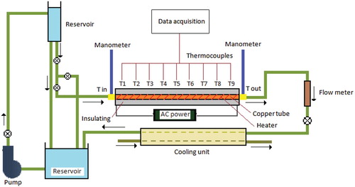
The first reservoir is occupied with fluid and the pump is used in order to move the fluid to the second reservoir. The Reynolds valve is used to direct the fluid into the horizontal channel. The fluid is then passed through a quadrangular cross-section heat transfer channel with a steady heat flux. Nine sensors were installed to measure the temperature of the channel wall. Finally, nanofluid passes through the cooling heat exchanger to provide a fixed inlet temperature.

The flow loop contains a test step, a fluid reservoir, a pump for circulating the fluid, measuring tools for the flow, calming stage, cooling section, riser part, and thermocouples. The test step is comprised of a copper tube (8 mm inner diameter, 1 mm thickness, and 1000 mm length). A MULTI 5800 SICCE pump performed the circulation of the working fluid at 5800 l/h. The calming section is used to obtain a fully developed laminar flow and eliminate the entrance effects. Glass wool insulator is used to reduce the testing section’s heat loss. Inlet and outlet temperatures are also measured using thermocouples. The test section also includes nine SMT-160 thermocouples and two manometers to determine the wall temperature and pressure drop, respectively. Flow rate is also calculated by determination of the time spent on filling the graduated cylinder.

To measure the H, a steady heat flux was provided on the duct's wall by using an electrical heating element, while the fluid passes through the duct. The amount of heat flux is determined by calculating the applied electrical power. The heat transfer rate is calculated via subtracting the heat loss from the heat flux. On the other hands, the temperature changes are measured by using the thermocouples. Finally, the ratio of the heat transfer rate was divided by the temperature range to obtain the H. The details of the equations employed to calculate the H have been described in previous works (Pourfayaz et al., 2018). The error amount was about 2.0%. Various Re, Pr, and x are investigated in this study (see Table 1). These dimensionless groups obtain from properties of the applied nanofluid. All experimental measurements were attached in Table S1 of supplementary content.

Table 1. Input parameters’ ranges.

X of nanofluid	Range of Re	Range of Pr	Range of H	No. of samples
0	456–743.6	5.007–6.483	61.34–886.63	63
0.0005	481–725	4.81–6.18	69.48–888.7	81
0.0007	508.3–674.5	4.48–5.75	82.15–904.95	63
0.002	522.5–700.64	3.99–5.09	80.11–1064.9	63

4. Models implementation

4.1. Preprocessing procedure

Three intelligent algorithms of MLP-ANN, ANFIS, and LSSVM were utilized to develop predictive models using MATLAB 2014, to obtain nanofluids’ H which is highly dependent to Re, Pr, and x, respectively. 270 experimental data points obtained using the experimental setup introduced in the previous section and employed in the development of the predictive models. The total dataset is classified into train (75%) and test (25%) subsections. The training dataset is employed to determination the corresponding parameters of the proposed predictive models, while the testing dataset determines is used to investigate the accuracy of the proposed models’ predictions. The experimental data points have to be homogenized first: (22) $D_n=2\frac{D-D_{min}}{D_{max}-D_{min}}-1$(22) where D represents the variable value. n stands as normalized value, min represents the minimum value, and max states the maximum value of the variable D. In this study, H is the target output and is defined as the function of Re, Pr, and x, respectively.

4.2. Model development

4.2.1. MLP-ANN

The overall output parameter of the proposed MLP-ANN is given as follows: (23) $M=\sum _{i=1}^n\left(W_{3i}\frac{1}{1+e^{-\left(x_i{W}_i\right)}}\right)+b_3$(23) where W_i, n, W_i,3, and b₃ represent the hidden layer neurons’ weight vector for in the number of hidden layer’s neurons, output layer neurons’ weight vector, and the bias term, respectively.

Optimum parameter values are obtained based on the adjustment of the corresponding weight factors and bias term. The following error function is applied to the optimization process of the MLP-ANN related parameters: (24) $E=\sum _j\sum _i\left(r_i^j-o_i^{j,l}\right)$(24) where j represents number of training dataset’s data points, $o_i^{j,l}$ is the first layer’s ith neuron’s output, and $r_i^j$ denotes the ith real value of the jth data point. Optimizing process is also carried out using the Levenberg-Marquardt algorithm.

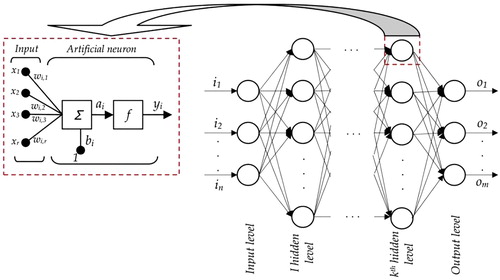
 Figure 2 represents the schematic configuration of the MLP-ANN. Performance of the proposed network is given in Figure S1 of the supplementary data. In addition, bias and weight values of the suggested structure were presented in Table S2 of supplementary data.

Figure 2. Schematic algorithm of multi-layer perceptron artificial neural network (MLP-ANN).

4.2.2. ANFIS

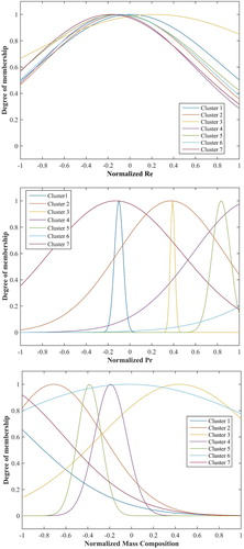
Figure 3 demonstrates an overview of an ANFIS configuration. ANFIS parameters were trained using the particle swarm optimization (PSO) method. The following formulation gives the total ANFIS elements amount to be obtained: (25) $N_T=N_c\cdot N_v\cdot N_{MF}$(25) where N_c, N_v, and N_MF represent numbers of clusters, variables, and membership function parameters, respectively. The Gaussian MF with two MF parameters (i.e. Z and σ²) is employed in this study. Four variables of H, Re, Pr, and x were introduced to the ANFIS strategy and primary number of clusters is set to 7. Therefore, there are 56 ANFIS parameters to be determined during the process of model development. Trained MF for each input parameter is given in Figure 4.

Figure 3. Construction of typical ANFIS.

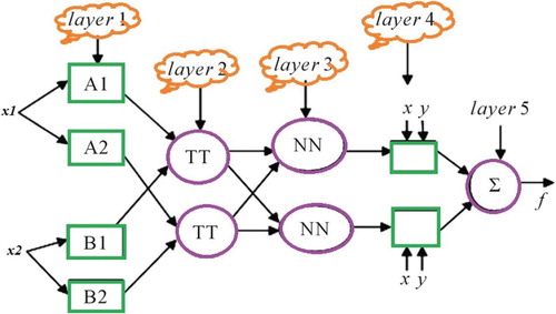
Figure 4. Trained variables of fuzzy inference system for inputs.

Root MSE (RMSE), given by the following formulation, is used as the cost function in the PSO method: (26) $\text{RMSE}={\left(\frac{1}{N}\sum _{i=1}^N{\left(H_i^{\exp .}-H_i^{\text{cal}\text{.}}\right)}^2\right)}^{0.5}$(26)

ANFIS model performance is given in Figure S2 of the supplementary data which represents the RMSE values for each iteration.

4.2.3. LSSVM

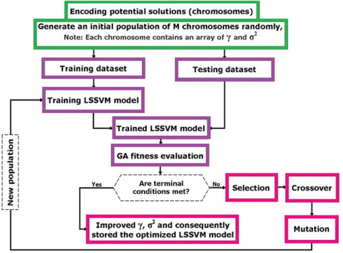
There are two adaptable elements in LSSVM configuration. These parameters are the regulation parameter (γ), and the kernel parameter (σ² from the RBF formulation). The LSSVM strategy employs the PSO method to specify the desired output (schematically overviewed in Figure 5).

Figure 5. Integration of GA with LSSVM, GA-LSSVM.

4.3. Models’ evaluation

Different statistical parameters including MSE, average relative deviation (ARD%), standard deviation (STD), and R² are employed to evaluate the predicted values of the H. The mentioned criterions are defined as follows: (27) $\text{MSE}=\frac{1}{N}\sum _{i=1}^N(H_i^{\exp .}-H_i^{\text{cal}\text{.}}{)}^2$(27) (28) $\text{ARD}\left(\mathrm{\%}\right)=\frac{100}{N}\sum _{i=1}^N\frac{|H_i^{\text{exp}\text{.}}-H_i^{\text{cal}\text{.}}|}{H_i^{\text{exp}\text{.}}}$(28) (29) $\text{STD}={\left(\frac{1}{N-1}\sum _{i=1}^N{\left(H_i^{\text{exp}\text{.}}-H_i^{\text{cal}\text{.}}\right)}^2\right)}^{0.5}$(29) (30) $R^2=1-\frac{{\sum }_{i=1}^N{\left(H_i^{\text{exp}\text{.}}-H_i^{\text{cal}\text{.}}\right)}^2}{{\sum }_{i=1}^N{\left(H_i^{\text{exp}\text{.}}-{\overline{H}}^{\text{exp}}\right)}^2}$(30)

5. Results and discussion

H estimation as a function of Re, Pr, and x is investigated using three intelligent algorithms (i.e. MLP-ANN, ANFIS, and LSSVM) employing an experimental dataset consisting of a total number of 270 data points. Table 2 provides detailed information on all the proposed models (i.e. MLP-ANN, ANFIS, and LSSVM).

Models’ performance and reliability were evaluated using different graphical approaches. The predicted and experimental values are compared and illustrated in Figure 6, where all three models suitably follow the trend of experimental H values. Regression plot of the predicted and experimental values for all three predictive models is depicted in Figure 7 from which an acceptable agreement of the predicted and the experimental values is concluded, since most of the data points are closely located in the vicinity of the unit slope line (Y = X). The best fitting lines resulted from linear regression of experimental and predicted values are also reported in Figure 9(a)–(c).

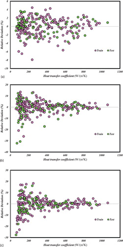
Another graphical approach is implemented regarding the deviation of the predicted H from their corresponding experimental values. Figure 8 represents the deviation plot for all three proposed models. The LSSVM strategy seems to have lower deviation due to higher accumulated data points near zero line. ARD percentage values of 4.2, 5.6, and 1.4 are obtained for MLP-ANN, ANFIS, and LSSVM strategies, respectively.

Table 2. The detailed specifications of the proposed smart predictive approaches.

LSSVM		ANFIS		MLP-ANN
Type	Value/comment	Type	Value/comment	Type	Value/comment
Kernel function	RBF	Membership Function	Gaussian	No. Input neuron layer	3
γ	4532.65	No. of MF parameters	56	No. Hidden neuron layer	8
σ^2	1.0324	No. of clusters	7	No. Output neuron layer	1
Number of data used for training	203	Number of data used for training	203	Hidden layer activation function	Logsig
Number of data used for testing	67	Number of data used for testing	67	Output layer activation function	Purelin
Population size	100	Population size	50	Optimization method	Levenberg-Marquardt
Iteration	1000	Iteration	1000	Number of data used for training	203
C1	1	C1	1	Number of data used for testing	67
C2	2	C2	2	Number of max iterations	1000

Figure 6. The obtained experimentally values of conductive H in comparison to proposed forecasting models: (a) LSSVM, (b) ANFIS, (c) MLP-ANN.

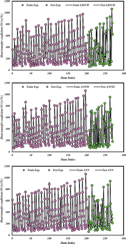
Figure 7. The Regression plot of obtained experimentally values of conductive H in comparison to proposed forecasting models: (a) LSSVM, (b) ANFIS, (c) MLP-ANN.

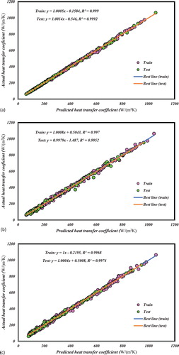
Figure 8. The obtained Relative deviations of experimentally values of conductive H in comparison to proposed forecasting models: (a) LSSVM, (b) ANFIS, (c) MLP-ANN.

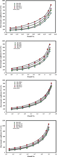
The dependence of the H on the Re and Pr for different x is illustrated in Figures 9–11 for the proposed models. As shown in Figures 9–11, experimental data points demonstrate that at constant Pr, increasing Re results in higher H values in all nanoparticle compositions. The same trend is observed for the case of constant Re and increasing the Pr. All proposed models followed the same trend which indicates the validity of the predicted values by the proposed models. These figures also indicate that Pr variations lead to larger H variations that is completely in agreement with the larger r reported for the Pr in Table 4.

Figure 9. Comparison of experimentally measured and forecasted conductive H values by the LSSVM model at various Re.

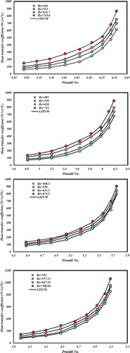
Figure 10. Comparison of experimentally measured and forecasted conductive H values by the ANFIS at various Re.

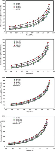
Figure 11. Comparison of experimentally measured and forecasted conductive H values by the MLP-ANN model at various Re.

Statistical error methodologies are also carried out to assess the predictive precision of the proposed designs. Table 3 represents the statistical error reports of training data, testing data, and total datasets for all three developed models. Calculated error parameters indicate that the proposed models are well capable of predicting the H as a function of Re, Pr, and x. The histogram of residuals is also depicted in Figure 12 in which the normal deviation distribution is concluded for all the proposed models regarding the bell-shaped histograms of the MLP-ANN, ANFIS, and LSSVM strategies.

Figure 12. Histogram diagram of residual data points for different implemented approaches.

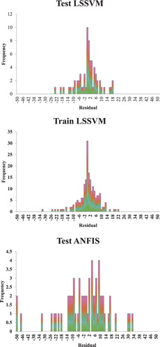
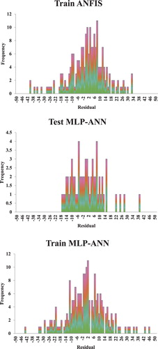
Table 3. Statistical error analyses.

Model		MSE	MRE	R^2	STD
LSSVM	Test	59.711	1.417	0.999	5.582
	Train	52.931	1.487	0.999	5.365
	Total	54.614	1.470	0.999	5.413
ANFIS	Test	303.156	5.584	0.995	12.449
	Train	168.716	3.702	0.997	8.643
	Total	202.077	4.169	0.997	9.764
MLP-ANN	Test	122.221	4.423	0.997	6.914
	Train	193.458	4.557	0.997	9.189
	Total	175.780	4.524	0.997	8.703

5.1. Outlier detection

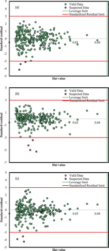
Experimental data points applied in the process of model development highly affects the credibility of a proposed model (Rousseeuw & Leroy, 2005). Outliers are individual or group of datum/data that behave differently from the majority of data points. Therefore, reliable model development requires the detection and exclusion of potential outlying data points in a set of available data points. The leverage analysis is employed in this study to determine possible outliers. Potential outlying candidates can be detected using the Williams plot (i.e. the plot of standardized residuals against the hat value). The diagonal parameters of the hat matrix are the Hat values and calculated as follows: (31) $H=X(X^{T}X{)}^{-1}{X}^T$(31) X shows a (n × k) dimensioned matrix where n and k are data points and input elements numbers, respectively. Feasible region is a squared area which is restricted by defining cut-off set point on the vertical axis and a warning leverage value on the horizontal axis. Warning leverage is: (32) $H^{\ast }=3\frac{k+1}{n}$(32)

A cut-off value of 3 is recommended for the standardized residual (R). Feasible region is therefore, restricted by $R=\pm 3$ lines on the vertical axis and H = 0 and H = H* on the horizontal axis. Outlying data points are positioned outer of the feasible area. A William’s plot is illustrated in Figure 13 indicating that most of the data points are positioned inner the feasible area except for 3, 4, and 3 data points for the MLP-ANN, ANFIS, and LSSVM models, respectively.

Figure 13. William’s plot for: (a) LSSVM, (b) ANFIS, (c) MLP-ANN.

5.2. Sensitivity analysis

Sensitivity analysis effectively determines the effects of each parameter on the target variable, regarding r ranging from −1 to +1. Higher absolute r value implies the higher impact of the related element on the aim variable. Positive and negative r values imply that increasing the corresponding parameter results in increasing and decreasing of the target variable, respectively. The r is mathematically given by the following expression: (33) $r=\frac{{\sum }_{i=1}^N\left(X_{k,i}-{\overline{X}}_k\right)\left(y_i-\overline{y}\right)}{\sqrt{{\sum }_{i=1}^N{\left(X_{k,i}-{\overline{X}}_k\right)}^2{\sum }_{i=1}^N{\left(y_i-\overline{y}\right)}^2}}$(33) r for each affecting parameters of Re, Pr, and x are reported in Table 4, where the Pr is found to be the most effective parameter on the H with a r of 0.524 and the x of nanofluid shows the lowest effects on the H with a 0.125 r.

Table 4. Sensitivity analysis of the input parameters.

	Re	Pr	X
r	0.168	0.524	0.125

6. Conclusion

Three intelligent algorithms (i.e. MLP-ANN, ANFIS, and LSSVM) were employed to correlate the H of a SiO₂/water nanofluid in a quadrangular cross-section channel. The predictive models are developed based on training the intelligent algorithms using experimentally measured data points to determine the H.

• Graphical and numerical error analyses were employed to determine the models’ ability in predicting the H. Graphical error analysis demonstrated that the predicted values are appropriately aligned with the trends observed in experiments. R² values were 0.999 (LSSVM), 0.997 (ANFIS), and 0.997 (MLP-ANN). These values indicate that all three models are capable of accurate prediction of the H. However, the LSSVM revealed a better performance regarding the lowest MSE value of 55.614 compared to 202.077 and 175.780 for ANFIS and MLP-ANN models, respectively.

• An outlier detection examination is also carried out to exclude the doubtful data points and increasing the credibility of the proposed modes where 3, 4 and 3 outlying data points were determined for LSSVM, ANFIS, and MLP-ANN designs, respectively.

• The sensitivity analysis also indicated the highest impact of the Pr on H with a r of 0.524 compared to that of 0.168 and 0.125 for Re and x of the nanofluid, repectively.

• These suggested approaches can apply for other nanofluid systems in order to investigate heat transfer performance in different types of heat exchangers.

Disclosure statement

No potential conflict of interest was reported by the authors.

ORCID

Ali J. Chamkha http://orcid.org/0000-0002-8335-3121

References

- Ahmadi, M. H., Nazari, M. A., Ghasempour, R., Madah, H., Shafii, M. B., & Ahmadi, M. A. (2018). Thermal conductivity ratio prediction of Al2O3/water nanofluid by applying connectionist methods. Colloids and Surfaces A: Physicochemical and Engineering Aspects, 541, 154–164.
- Akbarian, E., Najafi, B., Jafari, M., Faizollahzadeh Ardabili, S., Shamshirband, S., & Chau, K. (2018). Experimental and computational fluid dynamics-based numerical simulation of using natural gas in a dual-fueled diesel engine. Engineering Applications of Computational Fluid Mechanics, 12(1), 517–534.
- Amin, T. E., Roghayeh, G., Fatemeh, R., & Fatollah, P. (2015). Evaluation of nanoparticle shape effect on a nanofluid based flat-plate solar collector efficiency. Energy Exploration & Exploitation, 33(5), 659–676.
- Baghban, A., Ahmadi, M. A., Pouladi, B., & Amanna, B. (2015a). Phase equilibrium modeling of semi-clathrate hydrates of seven commonly gases in the presence of TBAB ionic liquid promoter based on a low parameter connectionist technique. The Journal of Supercritical Fluids, 101, 184–192.
- Baghban, A., Ahmadi, M. A., & Shahraki, B. H. (2015b). Prediction carbon dioxide solubility in presence of various ionic liquids using computational intelligence approaches. The Journal of Supercritical Fluids, 98, 50–64.
- Baghban, A., Bahadori, M., Rozyn, J., Lee, M., Abbas, A., Bahadori, A., & Rahimali, A. (2016). Estimation of air dew point temperature using computational intelligence schemes. Applied Thermal Engineering, 93, 1043–1052.
- Baghban, A., Jalali, A., Shafiee, M., Ahmadi, M. H., & Chau, K. (2019). Developing an ANFIS-based swarm concept model for estimating the relative viscosity of nanofluids. Engineering Applications of Computational Fluid Mechanics, 13(1), 26–39.
- Barbés, B., Páramo, R., Blanco, E., Pastoriza-Gallego, M. J., Piñeiro, M. M., Legido, J. L., & Casanova, C. (2013). Thermal conductivity and specific heat capacity measurements of Al2O3 nanofluids. Journal of Thermal Analysis and Calorimetry, 111(2), 1615–1625.
- Bhoopal, R. S., Sharma, P. K., Singh, R., & Beniwal, R. S. (2013). Applicability of artificial neural networks to predict effective thermal conductivity of highly porous metal foams. Journal of Porous Media, 16(7), 585–596.
- Chau, K. W., & Jiang, Y. W. (2002). Three-dimensional pollutant transport model for the Pearl River Estuary. Water Research, 36(8), 2029–2039.
- Das, S. K., Putra, N., Thiesen, P., & Roetzel, W. (2003). Temperature dependence of thermal conductivity enhancement for nanofluids. Journal of Heat Transfer, 125(4), 567–574.
- Esfe, M. H., Arani, A. A. A., Badi, R. S., & Rejvani, M. (2018). ANN modeling, cost performance and sensitivity analyzing of thermal conductivity of DWCNT–SiO2/EG hybrid nanofluid for higher heat transfer. Journal of Thermal Analysis and Calorimetry, 131(3), 2381–2393.
- Gandomkar, A., Saidi, M. H., Shafii, M. B., Vandadi, M., & Kalan, K. (2017). Visualization and comparative investigations of pulsating ferro-fluid heat pipe. Applied Thermal Engineering, 116, 56–65.
- Gurav, P., Naik, S. S., Ansari, K., Srinath, S., Kishore, K. A., Setty, Y. P., & Sonawane, S. (2014). Stable colloidal copper nanoparticles for a nanofluid: Production and application. Colloids and Surfaces A: Physicochemical and Engineering Aspects, 441, 589–597.
- Hemmati-Sarapardeh, A., Shokrollahi, A., Tatar, A., Gharagheizi, F., Mohammadi, A. H., & Naseri, A. (2014). Reservoir oil viscosity determination using a rigorous approach. Fuel, 116, 39–48.
- Hemmati-Sarapardeh, A., Varamesh, A., Husein, M. M., & Karan, K. (2018). On the evaluation of the viscosity of nanofluid systems: Modeling and data assessment. Renewable and Sustainable Energy Reviews, 81, 313–329.
- Huminic, G., & Huminic, A. (2012). Application of nanofluids in heat exchangers: A review. Renewable and Sustainable Energy Reviews, 16(8), 5625–5638.
- Hung, T.-C., Yan, W.-M., Wang, X.-D., & Chang, C.-Y. (2012). Heat transfer enhancement in microchannel heat sinks using nanofluids. International Journal of Heat and Mass Transfer, 55(9), 2559–2570.
- Ilyas, S. U., Pendyala, R., & Narahari, M. (2017). Stability and thermal analysis of MWCNT-thermal oil-based nanofluids. Colloids and Surfaces A: Physicochemical and Engineering Aspects, 527, 11–22.
- Islam, M. R., Shabani, B., Rosengarten, G., & Andrews, J. (2015). The potential of using nanofluids in PEM fuel cell cooling systems: A review. Renewable and Sustainable Energy Reviews, 48, 523–539.
- Jang, J.-S. R., Sun, C.-T., & Mizutani, E. (1997). Neuro-fuzzy and soft computing-a computational approach to learning and machine intelligence [Book Review]. IEEE Transactions on Automatic Control, 42(10), 1482–1484.
- Kalogirou, S. A. (2000). Applications of artificial neural-networks for energy systems. Applied Energy, 67(1), 17–35.
- Khanjari, Y., Pourfayaz, F., & Kasaeian, A. B. (2016). Numerical investigation on using of nanofluid in a water-cooled photovoltaic thermal system. Energy Conversion and Management, 122, 263–278.
- Kurt, H., & Kayfeci, M. (2009). Prediction of thermal conductivity of ethylene glycol–water solutions by using artificial neural networks. Applied Energy, 86(10), 2244–2248.
- Lee, K. H. (2004). First course on fuzzy theory and applications (Vol. 27). Berlin: Springer Science & Business Media.
- Lee, S., Choi, S.-S., Li and, S., & Eastman, J. A. (1999). Measuring thermal conductivity of fluids containing oxide nanoparticles. Journal of Heat Transfer, 121(2), 280–289.
- Lenin, R., & Joy, P. A. (2017). Role of base fluid on the thermal conductivity of oleic acid coated magnetite nanofluids. Colloids and Surfaces A: Physicochemical and Engineering Aspects, 529, 922–929.
- Lu, G., Duan, Y.-Y., & Wang, X.-D. (2014). Surface tension, viscosity, and rheology of water-based nanofluids: A microscopic interpretation on the molecular level. Journal of Nanoparticle Research, 16(9), 2564.
- Lu, G., Wang, X.-D., & Duan, Y.-Y. (2016). A critical review of dynamic wetting by complex fluids: From Newtonian fluids to non-Newtonian fluids and nanofluids. Advances in Colloid and Interface Science, 236, 43–62.
- Masuda, H., Ebata, A., & Teramae, K. (1993). Alteration of thermal conductivity and viscosity of liquid by dispersing ultra-fine particles. Dispersion of Al2O3, SiO2 and TiO2 ultra-fine particles.
- Moghadassi, A., Masoud Hosseini, S., Henneke, D., & Elkamel, A. (2009). A model of nanofluids effective thermal conductivity based on dimensionless groups. Journal of Thermal Analysis and Calorimetry, 96(1), 81–84.
- Mohamadian, F., Eftekhar, L., & Haghighi Bardineh, Y. (2018). Applying GMDH artificial neural network to predict dynamic viscosity of an antimicrobial nanofluid. Nanomedicine Journal, 5(4), 217–221.
- Mohanraj, M., Jayaraj, S., & Muraleedharan, C. (2012). Applications of artificial neural networks for refrigeration, air-conditioning and heat pump systems—A review. Renewable and Sustainable Energy Reviews, 16(2), 1340–1358.
- Mou, B., He, B.-J., Zhao, D.-X., & Chau, K. (2017). Numerical simulation of the effects of building dimensional variation on wind pressure distribution. Engineering Applications of Computational Fluid Mechanics, 11(1), 293–309.
- Nasiri, M., Etemad, S. G., & Bagheri, R. (2011). Experimental heat transfer of nanofluid through an annular duct. International Communications in Heat and Mass Transfer, 38(7), 958–963.
- Nasrin, R., & Alim, M. A. (2014). Semi-empirical relation for forced convective analysis through a solar collector. Solar Energy, 105, 455–467.
- Nazari, M. A., Ghasempour, R., Ahmadi, M. H., Heydarian, G., & Shafii, M. B. (2018). Experimental investigation of graphene oxide nanofluid on heat transfer enhancement of pulsating heat pipe. International Communications in Heat and Mass Transfer, 91, 90–94.
- Nikravesh, M., Zadeh, L. A., & Aminzadeh, F. (2003). Soft computing and intelligent data analysis in oil exploration (Vol. 51). Amsterdam: Elsevier.
- Oh, D.-W., Jain, A., Eaton, J. K., Goodson, K. E., & Lee, J. S. (2008). Thermal conductivity measurement and sedimentation detection of aluminum oxide nanofluids by using the 3ω method. International Journal of Heat and Fluid Flow, 29(5), 1456–1461.
- Öztop, H. F., Estellé, P., Yan, W.-M., Al-Salem, K., Orfi, J., & Mahian, O. (2015). A brief review of natural convection in enclosures under localized heating with and without nanofluids. International Communications in Heat and Mass Transfer, 60, 37–44.
- Pourfayaz, F., Sanjarian, N., Kasaeian, A., Razi Astaraie, F., Sameti, M., & Nasirivatan, S. (2018). An experimental comparison of SiO2/water nanofluid heat transfer in square and circular cross-section channels. Journal of Thermal Analysis and Calorimetry, 131(2), 1577–1586.
- Ramezanizadeh, M., Ahmadi, M. A., Ahmadi, M. H., & Nazari, M. A. (2018). Rigorous smart model for predicting dynamic viscosity of Al2O3/water nanofluid. Journal of Thermal Analysis and Calorimetry. doi: 10.1007/s10973-018-7916-1
- Ramezanizadeh, M., Alhuyi Nazari, M., Ahmadi, M. H., & Chau, K. (2019). Experimental and numerical analysis of a nanofluidic thermosyphon heat exchanger. Engineering Applications of Computational Fluid Mechanics, 13(1), 40–47.
- Rosenblatt, F. (1962). Principles of neurodynamics: Perceptrons and the theory of brain mechanisms. Washington, DC: Spartan.
- Rousseeuw, P. J., & Leroy, A. M. (2005). Robust regression and outlier detection (Vol. 589). New York City, NY: John Wiley & Sons.
- Rumelhart, D. E., Hinton, G. E., & Williams, R. J. (1962). Learning internal representations by error propagation. La Jolla, CA: California Univ San Diego La Jolla Inst for Cognitive Science.
- Saeedinia, M., Akhavan-Behabadi, M. A., & Nasr, M. (2012). Experimental study on heat transfer and pressure drop of nanofluid flow in a horizontal coiled wire inserted tube under constant heat flux. Experimental Thermal and Fluid Science, 36, 158–168.
- Safari, H., Nekoeian, S., Shirdel, M. R., Ahmadi, H., Bahadori, A., & Zendehboudi, S. (2014). Assessing the dynamic viscosity of Na–K–Ca–Cl–H2O aqueous solutions at high-pressure and high-temperature conditions. Industrial & Engineering Chemistry Research, 53(28), 11488–11500.
- Sahin, B., Gültekin, G. G., Manay, E., & Karagoz, S. (2013). Experimental investigation of heat transfer and pressure drop characteristics of Al2O3–water nanofluid. Experimental Thermal and Fluid Science, 50, 21–28.
- Sarkar, J. (2011). A critical review on convective heat transfer correlations of nanofluids. Renewable and Sustainable Energy Reviews, 15(6), 3271–3277.
- Suykens, J. A., Vandewalle, J., & De Moor, B. (2001). Optimal control by least squares support vector machines. Neural Networks, 14(1), 23–35.
- Vajjha, R. S., Das, D. K., & Kulkarni, D. P. (2010). Development of new correlations for convective heat transfer and friction factor in turbulent regime for nanofluids. International Journal of Heat and Mass Transfer, 53(21), 4607–4618.
- Valinataj-Bahnemiri, P., Ramiar, A., Manavi, S. A., & Mozaffari, A. (2015). Heat transfer optimization of two phase modeling of nanofluid in a sinusoidal wavy channel using artificial bee colony technique. Engineering Science and Technology, an International Journal, 18(4), 727–737.
- Wang, B., Wang, X., Lou, W., & Hao, J. (2012). Thermal conductivity and rheological properties of graphite/oil nanofluids. Colloids and Surfaces A: Physicochemical and Engineering Aspects, 414, 125–131.
- Wu, C. L., & Chau, K. W. (2006). Mathematical model of water quality rehabilitation with rainwater utilization: A case study at Haigang. International Journal of Environment and Pollution, 28, 534–545.
- Yang, L., Du, K., & Zhang, X. (2017). A theoretical investigation of thermal conductivity of nanofluids with particles in cylindrical shape by anisotropy analysis. Powder Technology, 314, 328–338.
- Zadeh, L. A. (1965). Fuzzy sets. Information and Control, 8(3), 338–353.
- Zarei, K., Atabati, M., & Moghaddary, S. (2013). Predicting the heats of combustion of polynitro arene, polynitro heteroarene, acyclic and cyclic nitramine, nitrate ester and nitroaliphatic compounds using bee algorithm and adaptive neuro-fuzzy inference system. Chemometrics and Intelligent Laboratory Systems, 128, 37–48.
- Zhao, G., Jian, Y., & Li, F. (2016). Streaming potential and heat transfer of nanofluids in parallel plate microchannels. Colloids and Surfaces A: Physicochemical and Engineering Aspects, 498, 239–247.