A study on non-spherical cuttings transport in CBM well drilling by coupled CFD-DEM

ABSTRACT

Due to the specificity of coal rock containing CBM (coal bed methane), large-sized cuttings from coal bed drilling present abnormal appearances which make the transport of cuttings more troublesome. Simulations of the transport of large-sized and non-spherical drilling cuttings in the horizontal well-bore annulus possesses both theoretical challenges and engineering worth. In this work, a coupled CFD-DEM model is developed and a multi-sphere method is adopted to construct the non-spherical cuttings particles including cubic and long flaky particles. Validation with the experimental data reveals the well applicability of the developed CFD-DEM model. The movements as well as the sedimentations of cuttings are discussed in detail. The influences of fluid velocity and particle shapes on the transport efficiency of cuttings are studied and more attention is paid to flaky cuttings. The results show that, with a consistent equivalent volume, relatively good performance happens to the 20 mm spherical particles while local piled bed appears to the flaky particles; however, cuttings in cubic particles behave the worst. In the chosen conditions, transport efficiency drops dramatically when the volume fraction of the flaky cuttings exceeds 10%. Work in this paper is expected to be able to be applied to CBM drilling engineering.

KEYWORDS:

• CFD-DEM
• CBM drilling
• cuttings transport
• non-spherical particles
• well cleaning

1. Introduction

Because of the specificity of the coal stratum and the structural complexity of the coal bed methane (CBM) wells, non-spherical cuttings in a larger size are more often produced during the drilling process. These large drill cuttings will not only bring impact failures to both strings and the well-wall, but also generate local blockages which may cause serious downhole problems like the jamming of the drilling tools (Akbarian et al., 2018; Akhshik & Rajabi, 2018; Duan, Miska, Yu, Takach, & Ahmed, 2007). Moreover, in the next stage of CBM production, failing to discharge the cuttings in a timely way is likely to cut back gas production. Therefore, studies on the transport of drill cuttings is always meaningful for the CBM industry.

Much research has been done on the transport of cuttings in both vertical and directional wells over the last few decades. Tomren, Iyoho, and Azar (1986), as well as Ford, Peden, Oyeneyin, Gao, and Zarrough (1990), did an experimental study of cuttings moving in directional wells. Sanchez, Azar, Bassal, and Martins (1999) took the rotation of the drill pipe into account and studied the well-hole cleaning in the process of directional well drilling. Duan et al. (2007) did simulation work on cuttings transport in horizontal and inclined wells with a big angle, in which critical conditions including the CRV (critical re-suspension velocity), the CFV (critical fluid velocity), and the CDV (critical deposition velocity) are discussed in detail. Song, Guan, and Chen (2009) developed the analytic models of CFV for different moving patterns of cuttings. Kelessidis and Bandelis (2004) investigated flow patterns and CRV specific to the particles transported in coiled-tubing drilling. Ozbayoglu, Saasen, Sorgun, and Svanes (2010) used the empirical correlations to estimate the CFV for preventing the evolution of a cuttings bed. Akhshik and Rajabi (2018) used a CFD (computational fluid dynamics) -DEM (discrete element method) model to study cuttings transport in an aerated mud drilling process, wherein the parameters’ effects were determined by the transport efficiency of cuttings including liquid flow rate, annulus inclination angle, and pressure, as well as an air injection rate. Many other researchers focused on the fluids which are used to carry the drilled cuttings (Capo, Yu, Miska, Takach, & Ahmed, 2006; Chen et al., 2007; Li et al., 2013; Manzar & Shah, 2009; Ozbayoglu, Erge, & Ozbayoglu, 2018).

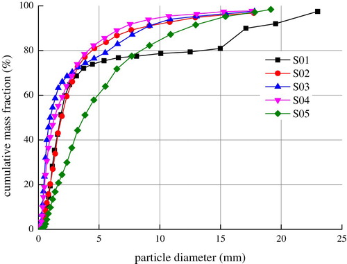
Detailed studies are being carried out all the time around the dynamics of particles moving in many sorts of fluids (Feng & Michaelides, 2004; Goyal & Derksen, 2012; Issakhov, Bulgakov, & Zhandaulet, 2019; Lee et al., 2008; Shao, Liu, Lin, Xu, & Yan, 2017). Referential significance is provided by these studies, however, due to their great computational consumption. Numerical methods used in these studies are rarely applied in calculations with a mass of particles or with large-scale models involved. Instead, the DEM is more frequently used in particle transport and it has also shown its superiority (Lu, Third, & Muller, 2015; Zeng, Li, & Zhang, 2018; Zhong, Yu, Liu, Tong, & Zhang, 2016). From the literature investigation, due to the complexity of the non-spherical particles concerning the forces effected by the shape and the computing consumption, the drill cuttings are usually treated as spherical particles and the size is limited to the millimeter level. A limited quantity of studies has been undertaken on the relatively larger particles of drilled cuttings. Walker and Li (2000) did experiments on the transport of particles whose diameter is up to 7 mm and results show a significant effect is produced by the particle size. Li and Wilde (2005) did some experimental work on the transport of cuttings and the effects from the density and size of the particle are studied, with the size of the particle being from 0.15 mm to 7.0 mm. But, on the other hand, very few people have paid much attention to the influences of the shape of the cuttings in the well-drilling process. Akhshik, Behzad, and Rajabi (2015) analyzed the influences of particle shape on particle transport by a CFD-DEM model. In their work, particles in different shapes including disc, cubic, and round particles were built and their results show the important role particle shape played in transport. Until now, more work needed to be conducted. From what we have investigated, on the one hand, cuttings from a CBM well by a PDC bit mostly appear to be long flakes. Figure 1(a) shows the sample of drilling cuttings. Due to the tremendous amount of cuttings for the whole well, which crosses diversified stratum containing various kinds of rocks on different depths, cuttings studied are taken from the target coal bed with vertical depth 810∼820 m in well ZP-1H. It is worth noting that the samples are manually processed and the oversized rock pieces are discarded. Figure 1(b) shows an oversized cuttings particle. On the other hand, the size of cuttings from a typical CBM well possesses a non-negligible range. Shown by Figure 2, the size of the cuttings in sample S01 concentrates upon two values: 2.2 and 21.0 mm. Combined with Figure 3, the mass fraction of cuttings smaller than 3 mm in samples S01∼S04 reaches 70% but 45% for S05; over 10% of cuttings are larger than 10 mm (21% for S01) and even exceed 23.0 mm.

Figure 1. Drill cuttings samples and oversized coal pieces discharged from well ZS-1H (>50 mm), flake shaped.

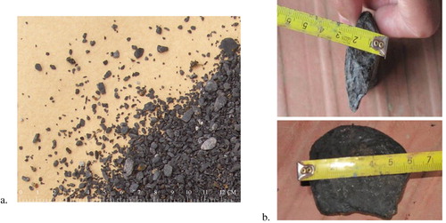
Figure 2. Grain size distribution for cuttings sample S01.

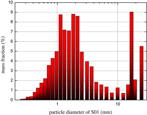
Figure 3. Cumulative weight of five cuttings samples.

Different from work done in the literature, focus is put on the transport of large-sized and non-spherical cuttings in this work, in which a multi-sphere particle model is added to the code of DEM. Simulations may provide a reference value for CBM well drilling, especially for choosing proper drilling fluid and setting operation parameters.

2. Model description

Governing equations for fluid and particles are given in this part, as well as the coupled algorithm of CFD-DEM. Based on the work of Kloss, Goniva, Hager, Amberger, and Pirker (2012), the open-source OpenFOAM is adopted to approximate the fluid field and a modified LIGGGHTS is used for calculating the particle motions, in which the multi-sphere model for non-spherical particles is added.

2.1. Fluid phase

In the coupled CFD-DEM, the incompressible fluid field is approximated by the CFD solver in OpenFOAM. The fluid is governed by the Navier-Stokes equations: (1) $\left.\begin{array}{c}{\rho }_f\left(\frac{\mathrm{\partial }\mathbf{u}}{\mathrm{\partial }t}+\mathbf{u}\cdot \mathbf{\nabla }\mathbf{u}\right)={\rho }_f\mathit{g}+\mathbf{\nabla }\cdot \mathit{\sigma }\\ \mathbf{\nabla }\cdot \mathbf{u}\mathbf{=}\mathbf{0}\end{array}\right\},\mathrm{\forall }t\text{> 0},$(1) where ${\rho }_f$, ${\mu }_f$ g, u, t and σ denote the fluid density, fluid viscosity, gravity vector, velocity, time, and stress tensor, respectively. σ is given by (2) $\mathit{\sigma }=-p\mathbf{1}\text{ +}{\mu }_f\left[\mathbf{\nabla }\mathbf{u}\text{ + }{\left(\mathbf{\nabla }\mathbf{u}\right)}^T\right]$(2)

The interactions between the particles and fluid are considered by S, which is the joint fluid force on the particles in the certain fluid cell containing particles, given as: (3) $S=\frac{1}{\mathrm{\Delta }V}\sum _{i=1}^n{\mathit{F}}_{f,i}$(3) where ΔV denotes the volume of the fluid cell; F_f,i denotes the force on the fluid cell and n denotes the particle quantity in the fluid cell.

2.2. Particle phase

The translation and rotation of the particles obeys Newton’s Law: (4) $\left.\begin{array}{l}{m}_i\frac{dU\left(t\right)}{\text{d}t}={\mathit{F}}_i\\ I_i\frac{d\mathrm{\Omega }\left(t\right)}{\text{d}t}={\mathit{T}}_i\end{array}\right\}\mathrm{\forall }\text{t> 0,}$(4) where m_i and I_i denote the mass and the moment of the inertia of the i_th particle respectively. F_i and T_i are the joint force and torque acting on the particle from the fluid, respectively. U(t)=dX(t)/dt and Ω(t) respectively denote the particle’s velocity and angular velocity.

The joint force F_i integrates the fluid drag force, fluid lift force, buoyancy force, contact forces with other particles, and the pressure gradient force. The fluid drag force is given as (Di Felice, 1994): (5) $F_{D,i}=0.5C_D{\rho }_f{A}_p\left(u_f-u_p\right)|u_f-u_p|{{\epsilon }_f}^{-\left(\chi +1\right)}$(5) where, $\chi =3.7-0.65\exp \left[\frac{-{\left(1.5-\mathrm{l}\mathrm{g}\mathrm{Re}\right)}^2}{2}\right]$; the drag coefficient C_D and Reynolds number Re are calculated by $C_D=(0.63+4.8/{\mathrm{Re}}^{0.5}{)}^2$ and $\mathrm{Re}=\frac{{\epsilon }_f{\rho }_f{d}_p|u_f-u_p|}{{\mu }_f}$. The lift force on the equivalent sphere is adopted for the multi-sphere particles, which is given as: (6) $F_L=\frac{1}{2}{\rho }_f|u_f-u_p{|}^2{A}_p{C}_L$(6) where the lift force coefficient can be got by $C_L=C_D{\sin }^2\beta \cos \beta$ and β is the angle between flow direction and the principle axis of particle.

The buoyancy force on the particle is given as: (7) ${\mathit{F}}^b=\frac{{\rho }_f}{{\rho }_p}{m}_s\mathbf{g}$(7) where the m_i denotes the overall mass of multi particles which is given below.

The torque exerted on the i_th particle when i_th particle contacts j_th particle is given by (8) ${\mathit{T}}_{ij}={\mathit{R}}_{ij}\times {\mathit{f}}_{ij,c}$(8) where, R_i is the vector from the contact point to the mass center of particle i; f_ij,c is the contact force between particle i and j.

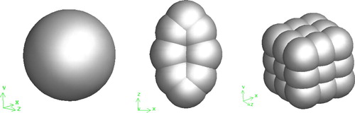
Due to the non-spherical appearance of the cuttings from the CBM well, the shape effects need to be considered for the cuttings transport simulation. In this work, multi spheres in the rigid connection are used to construct the non-spherical particles (Kruggel-Emden, Rickelt, Wirtz, & Scherer, 2008). Three non-spherical shapes, including a spherical particle, flaky particle, and cubic particle are taken in our simulation (Figure 4).

Figure 4. Particle models constructed by multi-sphere method.

For the non-spherical particle i built by identical spheres, the overall mass m_s, coordinates of the gravity center O_i and the inertia tensor I_i are given as (9) $m_s=\sum _{a=1}^N{m}_{s,a}$(9) (10) $O_i=\sum _{a=1}^N\left(O_{i,a}{m}_{s,a}\right)/m_s$(10) (11) $\begin{array}{rl}{I}_i& =\left[\begin{array}{c}\sum I_{i,a}+\sum m_{s,a}(O_{i,a,Y}^2+O_{i,a,Z}^2)\\ -\sum m_{s,a}{O}_{i,a,X}{O}_{i,a,Y}\\ -\sum m_{s,a}{O}_{i,a,X}{O}_{i,a,Z}\end{array}\right.\\ & \begin{array}{c}\sum m_{s,a}{O}_{i,a,X}{O}_{i,a,Y}\\ \sum I_{i,a}+\sum m_{s,a}(O_{i,a,X}^2+O_{i,a,Z}^2)\\ \sum m_{s,a}{O}_{i,a,Y}{O}_{i,a,Z}\end{array}\\ & \left.\begin{array}{c}\sum m_{s,a}{O}_{i,a,X}{O}_{i,a,Z}\\ \sum m_{s,a}{O}_{i,a,Y}{O}_{i,a,Z}\\ \sum I_{i,a}+\sum m_{s,a}(O_{i,a,X}^2+O_{i,a,Y}^2)\end{array}\right]\end{array}$(11) where N is the quantity of spheres; k denotes the k_th sphere in particle i; O_i,a,X, O_i,a,Y and O_i,a,Z are the distances from center of sphere k to the principle axes of the particle i in direction of X, Y, and Z, respectively.

2.3. Contact forces algorithm

The joint contact force ${\mathbf{F}}_{c,i}^p$ for two contacting particles consists of the normal contact force and tangential contact force, as well as their damping force (Di Renzo & Di Maio, 2004), which is shown in Figure 5. The joint contact force ${\mathbf{F}}_{c,i}^p$ is expressed as

Figure 5. Contact forces acting on particle i contacting with particle j.

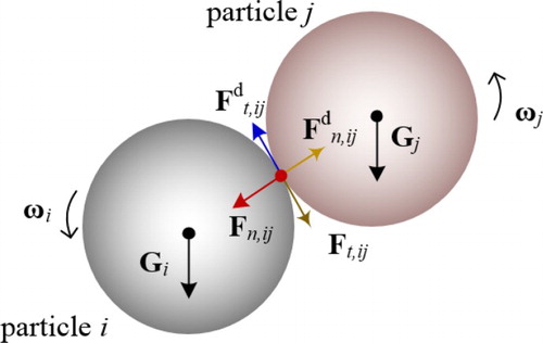
(12) ${\mathbf{F}}_{c,i}^p={\mathbf{F}}_{n,ij}+{\mathbf{F}}_{n,ij}^d+{\mathbf{F}}_{t,ij}+{\mathbf{F}}_{t,ij}^d$(12) where the subscript n and t denotes the normal component and tangential component respectively; superscript d denotes the damping force; subscript i and j denotes two contacting particles.

F_n,ij, ${\mathbf{F}}_{n,ij}^d$, F_t,ij and ${\mathbf{F}}_{t,ij}^d$ are given by Equation (13) ∼(16), respectively. (13) ${\mathbf{F}}_{n,ij}=\frac{4}{3}{E}^{\ast }\sqrt{R^{\ast }}{\delta }_{n,ij}^{3/2}$(13) where E* denotes equivalent Young’s modulus ($E^{\ast }=\left[\right(1-{\upsilon }_i^2)/E_i+(1-{\upsilon }_j^2)/E_j{]}^{-1}$), R* is the equivalent radius ($R^{\ast }=(2/d_p+2/d_q{)}^{-1}$), δ_n,ij is the normal overlap, E is the Young’s modulus, υ denotes Poisson ratio, d_i is the particle radius, the subscript i and j denote the particle i and particle j respectively. (14) ${\mathbf{F}}_{n,ij}^d=-2\sqrt{\frac{5}{6}}\frac{\ln e}{\sqrt{{(\ln e)}^2+{\pi }^2}}\sqrt{S_{n,ij}{m}^{\ast }}{\mathbf{v}}_{n,pq}$(14) where $S_{n,ij}=2E^{\ast }\sqrt{R^{\ast }{\delta }_{n,ij}}$ is the normal stiffness, m* is the equivalent particle mass ($m^{\ast }=[1/m_i+1/m_j{]}^{-1}$) composed by the mass of the contacting particles m_i and m_j, e denotes the coefficient of restitution, v_n,pq is the normal contact velocity. (15) ${\mathbf{F}}_{t,ij}=\left\{\begin{array}{ll}-{\delta }_{t,ij}{S}_{t,ij},& |{\mathbf{F}}_{t,ij}|<{\mu }_s{\mathbf{F}}_{n,ij}\\ {\mu }_s|{\mathbf{F}}_{n,ij}|\frac{{\text{v}}_{t,pq}}{|{\text{v}}_{t,pq}|},& |{\mathbf{F}}_{t,ij}|\ge {\mu }_s{\mathbf{F}}_{n,ij}\end{array}\right.$(15) (16) ${\mathbf{F}}_{t,ij}^d=-2\sqrt{\frac{5}{6}}\frac{\ln e}{\sqrt{{(\ln e)}^2+{\pi }^2}}\sqrt{S_{t,ij}{m}^{\ast }}{\text{v}}_{t,pd}$(16) where μ_s denotes the sliding friction coefficient and subscript t denotes the tangential component. The tangential stiffness S_t,ij is given as: (17) $S_{t,ij}=8G^{\ast }\sqrt{R^{\ast }{\delta }_{n,ij}}$(17) where the δ_t,ij is the overlap of two particles in tangential direction. Equivalent shear modulus G* is given by (18) $G^{\ast }=\left[\right(1-{\upsilon }_i^2)/G_i+(1-{\upsilon }_j^2)/G_j{]}^{-1}$(18)

2.4. CFD-DEM coupled algorithm

In the coupled CFD-DEM, the CFD solver in OpenFOAM is used to approximate the fluid field while the motions of particles are calculated by DEM in LIGGGHTS, which is illustrated by Figure 6. The communicating process contains the procedures below.

• By the CFD model, the continuity, momentum, and turbulence of the fluid are approximated until converged;

• On the basis of the particle VF in the cell where the particles locate, the fluid forces exerted on each particle are computed;

• The DEM solver approximates the particles’ positions and velocities until computation is converged;

• After one CFD time step, updated information of the particles is sent back to the CFD solver to calculate the VF and forces of fluid.

Figure 6. Coupling diagram of the CFD-DEM framework.

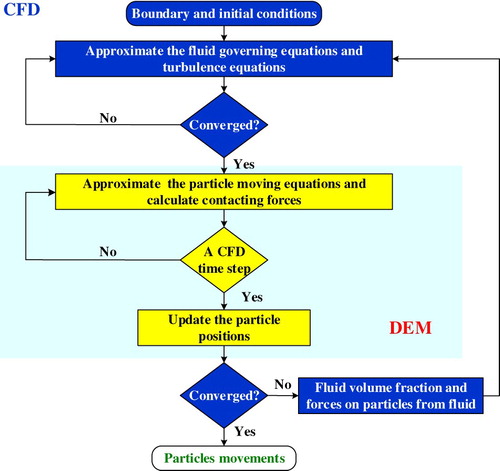
Circularly, the CFD solver once again iterates over a new time step until the solution converges.

3. Model validation

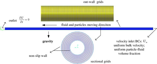
To guarantee the applicability of the coupled CFD-DEM model for the solid­–fluid interaction in cuttings transport, experimental data from our previous work (Shao, Yan, Bi, & Yan, 2017) is used to be compared. In Shao’s work, cuttings transport under varying conditions is experimentally studied and the analytical model of FCV V_c is verified. The cuttings used are also taken from the typical CBM well ZS-1H. Here we use the CFD-DEM to develop the corresponding simulation model from the experiments and make the comparison. A geometrically identical model is built with the external and internal diameter of the annulus being 140 and 63 mm respectively, and with horizontal length being 25.0 m. Moreover, properties for cuttings are taken with density being 2300 kg/m³, Poisson’s ratio being 0.25, shear modulus being 1.96 GPa and the sizes of particles being 2, 4, and 6 mm. The two shapes of particles taken in simulations, which are flaky particles and spherical particles, are shown in Figure 4. The inside fluid is water whose density is 1.0 g/cm³ and viscosity is 0.01 cm²/s. Figure 7 shows some experimental details. Cuttings particles are screened to shares in different sizes which are used for simulating the transport of cuttings in varying size. 2  and 4 mm cuttings are shown in the left and right part of Figure 7(a and b), which shows the experimental equipment including tubes, motor, vessels and data acquisition unit, and so on. Mesh and boundary conditions for a numerical simulation model can be found in Figure 8.

Figure 7. Experimental pictures: (a) cuttings particles in size of 2 mm for the left picture and 4 mm for the right; (b) experimental equipment.

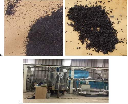
Figure 8. Verification model and mesh.

Like the experiments, a small value is taken initially for the inlet velocity of the fluid, and with accelerating the flow velocity, the particles in the annulus start moving from the idle state. Once the cuttings particles are all carried out with no local heap existing, the flow velocity is taken as the FCV V_c. Simulations are conducted for cuttings to size of 2, 4, and 6 mm respectively.

The critical velocities both from the experiments and simulations are given in Figure 9.

Figure 9. Results comparison between simulations and experiments.

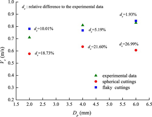
As shown by Figure 9, with the varying of particle size, the trend in the numerical results of V_c agrees with experimental values. On the whole, the critical value grows while the particle size rises. However, considerable differences exist for the spherical particles, whose average value for particles in three sizes reaches 22.44% lower than the experimental value. But on the upside, when long flaky particles are used for the cuttings phase, the average difference decreases to 5.71%, which is acceptable in engineering.

The validation cases indicate that the coupled CFD-DEM is competent for the simulation of the transport of cuttings and, furthermore, the flaky particles are more appropriate to take the place of cuttings in the numerical simulations.

4. Cuttings transport simulations

4.1. CFD-DEM model

According to the well logging and drilling data of well ZS-1, the whole well simulation model is built containing about 2490 thousand grids, which is shown in Figure 10. The grid size varies in a range of 0.005  to 0.05 m and the corresponding grid volume varies from 3.7e-8 to 1.3e-5 m³.

Figure 10. Numerical model and mesh for well ZS-1.

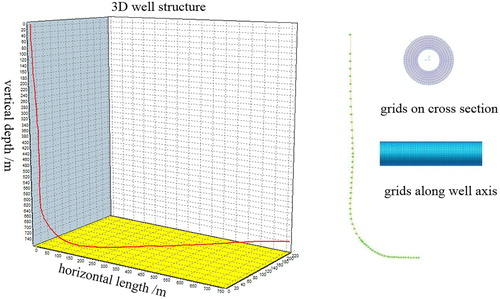
The 100.0 m-long horizontal part of the wellbore annulus is taken for discussion with casing as the outside well-wall and a drilling tube as the inside well-wall. The external diameter of the annulus is 15.24 cm; the internal diameter is 8.89 cm with no eccentricity. Structural grids are used and the mesh is similar to the validation model. Boundary conditions can be illustrated by Figure 8 with the fluid inlet and outlet be replaced by the bottom end and the top end of the well respectively. By the discharge rate of the drilling fluid being 15 L/s, the flow velocity in annulus can be deduced as 1.25 m/s, which is set as the initial inlet velocity. By the DPR (drill pipe rotary) 90 r/min, the rotary speed of the fluids near the internal wall is set to be 9.42 rad/s. Like the spherical particles and flaky particles, cubic particles in 20 mm equivalent diameter are built, shown by Figure 4. The k-ε turbulence model is adopted for the unsteady flow. By the AROP (average rate of penetration) of 28 min/m, the VF of the cuttings is deduced as 0.0724%, meaning the particle quantity flow is 1.1e-5m³/s and the particles are sequentially introduced on the inlet with a same velocity to that of drilling fluid. In order to be closer to the actual engineering case, besides the 20 mm particles, cuttings particles are mixed up with particles of a smaller size (2 mm). In section 5.2, the mass fraction of 20 mm particles in all is taken as 15%. The drilling fluid is water, whose properties can be found in the validation model. The turbulence intensity I can be got by I = 0.16Re^-1/8, which is given as 5.38%.

4.2. Fluid velocity in wellbore annulus containing large cuttings

Cuttings transport is studied for large non-spherical particles, which means cubic particles, spherical particles, and flaky particles in this work. Moving states and fluid fields in annulus are discussed.

Fluid velocity contours and vector diagram are given in Figure 11. As shown, for all three shaped particles, the flow fields in the upper part of annulus are relatively stable while for the cubic and flaky particles, flows in the lower part of annulus behave unstably, which is caused by disturbances from the local packed beds. That is to say, large-sized cubic particles and flaky particles are more easily to deposit and form local packed beds than spherical particles. The states of particles moving and depositing can be found in Figure 12, which shows obvious differences on the packed beds among cuttings in three shapes. In order to compare the details, three locations in the lower part of annulus are chosen to extract the detail data, which is indicated by Figure 13.

Figure 11. Drilling fluid velocity distribution in the annulus of the well containing cuttings in different shapes.

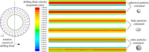
Figure 12. Deposition of large-sized cuttings with different shapes in well annulus space

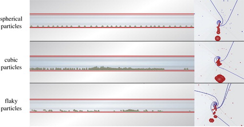
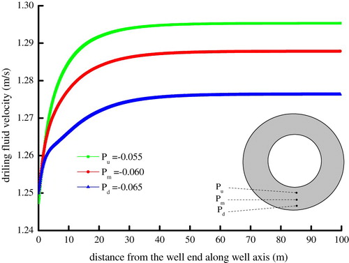
Figure 13. Trend of fluid velocity along the bottom of the annulus containing 20 mm spherical cuttings (P_u, P_m, P_d indicate three monitored lines in the lower part of the annulus along the well axis which are averagely chosen in the radial direction).

In Figure 12, compared to 2 mm particles, large-sized particles (20 mm) fail to be suspended in the fluids, but deposit or move along the bottom of the annulus. Spherical particles spread evenly along the bottom and move forward while most of the cubic particles are deposited on the lower part of the annulus and block the lower transport space. Differently, local packed beds appear for the flaky particles, but not as seriously as for the cubic particles. In addition, from the parallel vision with the well axis, the small particles can be carried out smoothly in suspension.

Compared with Figures 14 and 15, curves in Figure 13 are relatively smoother, which means the flow is steady at the same horizontal height in the lower part of the annulus and, moreover, spherical cuttings move evenly along the wellbore bottom. The smaller velocity of flow closer to the annulus bottom demonstrates a failed suspension of large-sized particles at the bottom and so it dose to other shaped particles.

Figure 14. Trend of fluid velocity along the bottom of the annulus containing 20 mm cubic cuttings.

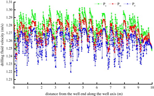
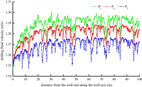
Figure 15. Trend of fluid velocity along the bottom of the annulus containing 20 mm flaky cuttings.

Shown by Figure 14, widely different with the spherical particles, the velocity of fluid containing large-sized cubic particles at the same horizontal height behaves much more unstably. Strong dispersion exists in the flow velocity along the axis of the well with the same distance to the wall. It can be explained by the deposits of the large-sized particles, where the packed cuttings beds along the bottom cause great disturbances to the flow. In other words, the fluid used in simulations has a poor capability to carry out the large-sized cubic cuttings.

Similarly, flow velocities of fluids containing large-sized flaky particles behave unstably, as given in Figure 15. Data dispersions mean disturbances are produced by the local packed beds along the bottom wall, formed by the deposited large-sized flaky particles. However, improvements are presented compared somewhat with the cubic particles.

Based on the above discussions, for large-sized particles in irregular particles, fluid demonstrates the best carrying capability for the spherical particles while also the worst for the cubic particles; this also means the flaky particles take the middle place.

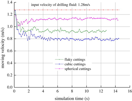
The average moving velocities of the particles versus time are given in Figure 16, which highlights the influence of the shape. From Figure 16, stable moving states are realized after the sufficient development of the field. The ratios of the moving speeds of three particles to the fluid velocity are 86.61%, 72.04%, and 62.65% for spherical particles, flaky particles, and cubic particles respectively. The result data reveals the double confirmation that the cubic cuttings are hardest to be carried out while the spherical particles are easiest to be transported. So, certain experience about the drilling engineering measures based on the spherical cuttings is risky to some degree.

Figure 16. Trend of average migration velocity of large-sized cuttings with time.

4.3. Influences of a fraction of large-sized and flaky cuttings

From the discussion above, the flaky particles are regarded as closest to the real cuttings samples. Keeping the total volume fraction of the cuttings in fluid as being fixed, we change the mass ratio of the large-sized and flaky particles (20 mm) to the small particles (2 mm). The mass ratio is taken as 1:3, 1:5, 1:10, 1:15, and 1:20 respectively. The moving speeds of all particles is extracted and the average value is calculated. As a result, the ratios of average moving speeds for cuttings containing large-sized flaky particles to the fluid velocity changing with the time are given in Figure 17.

Figure 17. Trend of the ratios between the velocities of cuttings and fluid versus time effected by the fraction of large-sized flaky cuttings.

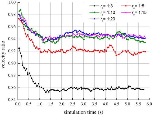
From Figure 17 it is obvious that, when the fraction of large-sized particles is larger, the velocity ratio will be smaller, which means a worse carrying capability for the fluid. With the largest fraction 1:3, the velocity ratio is smallest and with the decreasing of the fraction of large-sized particles, the cuttings move faster. However, once the fraction of the large-sized particles drops under 10%, the effect becomes no more evident.

5. Conclusions

With the developed CFD-DEM coupled model, the transport of cuttings containing non-spherical and large-sized particles in the well annulus are studied. From the work that has been done, the CFD-DEM model is confirmed to be applicable. As a result, some conclusions are drawn. For particles with the same volume, spherical particles are easiest to be carried out and flaky particles take second place; the cubic particles are hardest to be carried out. Moreover, the more large-sized particles contained in the cuttings, the harder the cuttings will be to be carried by the fluid; however, when the fraction of 20 mm flaky particles is less than 10%, the influence is much weakened.

Some limitations still exist in this work, such as the fact that although flaky particles square with the cuttings from a CBM well, they may be not suitable for cuttings from other kinds of wells. Improvements are still needed to be made on the methodologies; for example, lots of spheres are needed to build a precise non-spherical particle by the multi-sphere model, which may cause unaffordable computation consumption. Therefore, more work needs to be done to improve the computational methods in future.

Acknowledgments

The authors are grateful for the financial support of China Postdoctoral Science Foundation (grant number 2018M640665), National Natural Science Foundation of China (grant number 51804330), and National Natural Science Foundation of China (grant number 51875579).

Disclosure statement

No potential conflict of interest was reported by the authors.

ORCID

Bing Shao http://orcid.org/0000-0003-2436-8750

Additional information

Funding

The authors are grateful to the financial support of China Postdoctoral Science Foundation (grant number 2018M640665), National Natural Science Foundation of China (grant number 51804330) and National Natural Science Foundation of China (grant number 51875579).

References

- Akbarian, E., Najafi, B., Jafari, M., Ardabili, S. F., Shamshirband, S., & Chau, K.-W. (2018). Experimental and CFD-based numerical simulation of using natural gas in a dual-fuelled diesel engine. Engineering Applications of Computational Fluid Mechanics, 12(1), 517–534. doi: 10.1080/19942060.2018.1472670
- Akhshik, S., Behzad, M., & Rajabi, M. (2015). CFD–DEM model for simulation of non-spherical particles in hole cleaning process. Particulate Science and Technology, 33, 472–481. doi: 10.1080/02726351.2015.1010760
- Akhshik, S., & Rajabi, M. (2018). CFD-DEM modeling of cuttings transport in underbalanced drilling considering aerated mud effects and downhole conditions. Journal of Petroleum Science and Engineering, 160, 229–246. doi: 10.1016/j.petrol.2017.05.012
- Capo, J., Yu, M., Miska, S., Takach, N. E., & Ahmed, R. (2006). Particles transport with aqueous foam at intermediate inclined wells. SPE Drilling & Completion, 21(2), 99–107. doi: 10.2118/89534-PA
- Chen, Z., Ahmed, R. M., Miska, S., Takach, N., Yu, M., Pickell, M. B., & Hallman, J. H. (2007). Experimental study on particles transport with foam under simulated horizontal downhole conditions. SPE Drilling & Completion, 22(4), 304–312. doi: 10.2118/99201-PA
- Di Felice, R. (1994). The voidage function for fluid-particle interaction systems. International Journal of Multiphase Flow, 20(1), 153–159. doi: 10.1016/0301-9322(94)90011-6
- Di Renzo, A., & Di Maio, F. P. (2004). Comparison of contact-force models for the simulation of collisions in DEM-based granular flow codes. Chemical Engineering Science, 59(3), 525–541. doi: 10.1016/j.ces.2003.09.037
- Duan, M., Miska, S., Yu, M., Takach, N., & Ahmed, R. (2007). Critical conditions for effective sand-sized solids transport in horizontal and high-angle wells. SPE106707 presented at the production and operations Symposium, Oklahoma City, Oklahoma, USA.
- Feng, Z., & Michaelides, E. (2004). The immersed boundary-lattice boltzmann method for solving fluid-particles interaction problems. Journal of Computational Physics, 195(2), 602–628. doi: 10.1016/j.jcp.2003.10.013
- Ford, J. T., Peden, J. M., Oyeneyin, M. B., Gao, E., & Zarrough, R. (1990). Experimental investigation of drilled cuttings transport in inclined boreholes. SPE 20421 presented at the 65th Annual Technical Conference and Exhibition of the Society of Petroleum Engineers, New Orleans, LA, USA.
- Goyal, N., & Derksen, J. J. (2012). Direct simulations of spherical particles sedimenting in viscoelastic fluids. Journal of Non-Newtonian Fluid Mechanics, 183–184, 1–13. doi: 10.1016/j.jnnfm.2012.07.006
- Issakhov, A., Bulgakov, R., & Zhandaulet, Y. (2019). Numerical simulation of the dynamics of particle motion with different sizes. Engineering Applications of Computational Fluid Mechanics, 13(1), 1–25. doi: 10.1080/19942060.2018.1545253
- Kelessidis, V. C., & Bandelis, G. E. (2004). Flow patterns and minimum suspension velocity for efficient particles transport in horizontal and deviated wells in coiled-tubing drilling. SPE Drilling & Completion, 19(4), 213–227. doi: 10.2118/81746-PA
- Kloss, C., Goniva, C., Hager, A., Amberger, S., & Pirker, S. (2012). Models, algorithms and validation for opensource DEM and CFD-DEM. Progress in Computational Fluid Dynamics, 12(2/3), 140–152. doi: 10.1504/PCFD.2012.047457
- Kruggel-Emden, H., Rickelt, S., Wirtz, S., & Scherer, V. (2008). A study on the validity of the multi-sphere discrete element method. Powder Technology, 188, 153–165. doi: 10.1016/j.powtec.2008.04.037
- Lee, T. R., Chang, Y. S., Choi, J. B., Kim, D. W., Liu, W. K., & Kim, Y. J. (2008). Immersed finite element method for rigid body motions in the incompressible Navier-Stokes flow. Computer Methods in Applied Mechanics and Engineering, 197, 2305–2316. doi: 10.1016/j.cma.2007.12.013
- Li, X., Li, G., Song, W., Cui, G., Chen, J., & Tang, B. (2013). Research on hole cleaning in horizontal well with aerated underbalanced drilling. Science Technology and Engineering, 13(24), 7138–7142.
- Li, J., & Wilde, G. (2005). Effect of particle density and size on Solids transport and hole cleaning with coiled tubing. SPE 94187 presented at SPE/ICoTA coiled tubing Conference and Exhibition, Woodlands, Texas, USA.
- Lu, G., Third, J. R., & Muller, C. R. (2015). Discrete element models for non-spherical particles systems: From theoretical developments to applications. Chemical Engineering Science, 127, 425–465. doi: 10.1016/j.ces.2014.11.050
- Manzar, M. A., & Shah, S. N. (2009). Particle distribution and erosion during the flow of Newtonian and Non-Newtonian slurries in straight and coiled pipes. Engineering Applications of Computational Fluid Mechanics, 3(3), 296–320. doi: 10.1080/19942060.2009.11015273
- Ozbayoglu, E. M., Erge, O., & Ozbayoglu, M. A. (2018). Predicting the pressure losses while the drillstring is buckled and rotating using artificial intelligence methods. Journal of Natural Gas Science & Engineering, 56, 72–80. doi: 10.1016/j.jngse.2018.05.028
- Ozbayoglu, E. M., Saasen, A., Sorgun, M., & Svanes, K. (2010). Critical fluid velocities for removing particles bed inside horizontal and deviated wells. Petroleum Science and Technology, 28(1), 594–602. doi: 10.1080/10916460903070181
- Sanchez, R. A., Azar, J. J., Bassal, A. A., & Martins, A. L. (1999). Effect of drill pipe rotation on hole cleaning during directional-well drilling. SPE Journal, 4(2), 101–108. doi: 10.2118/56406-PA
- Shao, B., Liu, G. R., Lin, T., Xu, G. X., & Yan, X. Z. (2017). Rotational and orientation of irregular particles in viscous fluids using the gradient smoothed method (GSM). Engineering Application of Computational Fluid Mechanics, 11(1), 557–575. doi: 10.1080/19942060.2017.1329169
- Shao, B., Yan, Y., Bi, C., & Yan, X. (2017). Primary research on movement of big-sized cuttings in coal-bed methane wells by parallel computing using coupled CFD-DEM. Science Technology and Engineering, 17(15), 42–47.
- Song, X., Guan, Z., & Chen, S. (2009). Mechanics model of critical annular velocity for cuttings transportation in deviated well. Journal of China University Petroleum, 33(1), 53–56.
- Tomren, P. H., Iyoho, A. W., & Azar, J. J. (1986). Experimental study of cuttings transport in directional well. SPE Drilling Engineering, 1(1), 43–56. doi: 10.2118/12123-PA
- Walker, S., & Li, J. (2000). The effects of particle size, fluid rheology, and pipe eccentricity on particles transport. SPE 60755 presented at the SPE/ICoTA coiled tubing Roundtable held in Houston, TX, USA.
- Zeng, J., Li, H., & Zhang, D. (2018). Numerical simulation of proppant transport in hydraulic fracture with the upscaling CFD-DEM method. Journal of Natural Gas Science & Engineering, 33, 264–277. doi: 10.1016/j.jngse.2016.05.030
- Zhong, W., Yu, A., Liu, X., Tong, Z., & Zhang, H. (2016). DEM/CFD-DEM modeling of non-spherical particulate systems: Theoretical developments and applications. Powder Technology, 302, 108–152. doi: 10.1016/j.powtec.2016.07.010