Application of ANFIS and LSSVM strategies for estimating thermal conductivity enhancement of metal and metal oxide based nanofluids

Abstract

An extensive variety of chemical engineering processes include the transfer of heat energy. Since increasing the effective contact surface is known as one of the popular manners to improve the efficiency of heat transfer, the attention to the nanofluids has been attracted. Due to the difficulty and high cost of an experimental study, researchers have been attracted to fast computational methods. In this work, Adaptive neuro-fuzzy inference system and least square support vector machine algorithms have been applied as a comprehensive predictive tool to forecast the nanofluids thermal conductivity in terms of diameter, temperature, the thermal conductivity of the base fluid, the thermal conductivity of nanoparticle and volume fraction. To this end, a large and comprehensive experimental databank contains 1109 data points have been collected from reliable sources. The particle swarm optimization is utilized to reach the best structures of the proposed algorithms. A comprehensive statistical and graphical investigations are carried out to prove the accuracy and ability of proposed models. In addition, the comparisons outputs indicate that the least square support vector machine algorithm has the best performance among the existing correlations and Adaptive neuro-fuzzy inference system algorithms for forecasting thermal conductivity of different nanofluids.

KEYWORDS:

• Nanofluid
• thermal conductivity
• least square support vector machine algorithm
• Adaptive neuro-fuzzy inference system

Nomenclature

ANFIS	=	Adaptive neuro-fuzzy inference system
LSSVM	=	Least squares support vector machine
ANN	=	Artificial neural network
PSO	=	Particle swarm optimization
T	=	transposed matrix
µ	=	relation of total regression weight errors and single weights
αi	=	Lagrangian multiplier
ϕ(x)	=	nonlinear function
ω	=	weight
b	=	bias
ϒ	=	regularization parameter
ek	=	support value
K	=	kernel function
Z	=	Gaussian parameter
σ	=	Gaussian parameter
m	=	One of the resulting index of ANFIS
n	=	One of the resulting index of ANFIS
r	=	One of the resulting index of ANFIS
W	=	inertia weight
c	=	learning rate
R2	=	coefficient of determination
AARD	=	average absolute relative deviation
MSE	=	Mean squared error
STD	=	Standard deviation
H	=	Hat matrix
H*	=	The leverage limit
EG	=	Ethylene Glycol
EO	=	Engine oil
DI Water	=	Deionized Water
MEG	=	Ethylene glycol
CNT	=	Carbon nanotubes
MWCNT	=	Multi-walled Carbon nanotubes

1. Introduction

Owning to extensive applications of heat transfer phenomenon in different industrial instruments such as the cooling systems, compressor, evaporators, and boilers, it is well-known as a critical point. There is a direct relationship between the efficiency of such instruments and their requirement volume, which is significant for us to have economically process (Wen, Lin, Vafaei, & Zhang, 2009; Zalba, Marı´n, Cabeza, & Mehling, 2003). Furthermore, it should be noted that a kind of working fluid usually passes within such heat transfer devices through a pump or compressor and as the efficiency of heat transfer increases the required power consumption and thus processing cost decrease. Numerous studies have been implemented in order to improve heat transfer efficiency (Ebrahimnia-Bajestan, Moghadam, Niazmand, Daungthongsuk, & Wongwises, 2016; Mazumdar et al., 2016; Tomlinson, Manning, Schaefer, & Record, 2016). The improvement of effective surface, using microscale channels and vibration technique can be named as efforts that help to enhance the heat transfer efficiency. According to annually published articles, there are numerous attentions on nanofluid systems. Furthermore, the thermal conductivity property is known as a major factor in the improvement of heat transfer efficiency. the thermal conductivity property of some base fluids such as ethylene glycol (EG), water (H₂O) and different types of oil, some addition of nanoparticles to these fluids can increase their thermal conductivity (Eiamsa-ard & Wongcharee, 2018; Zeeshan, Shehzad, Ellahi, & Alamri, 2017). These nanoparticles give us the advantage of having a simple fluidized process and they solve some major problems, for example, the precipitation of particles, the blockage of channels, and erosion problems because of their nanosize structures.

The suspension of particles in a base fluid was introduced by Chol as an innovative aspect of nanofluilds (Chol, 1995). Furthermore, an interesting application of them was suggested in microchannels (Chein & Chuang, 2007). In recent years, numerous attempts have been done to estimate the nanofluids thermal conductivity utilizing mathematical and computational methods. Ghalambaz et al. investigated heat transfer convection of Cu-water nanofluids through a porous media parallelogrammic enclosure numerically by utilizion Tiwari model. They studied the effect of volume fraction of nanoparticles, inclination angle and porous media matrix on heat transfer (Ghalambaz, Sheremet, & Pop, 2015). Sheremet et al. used Buongiorno’ model to study free convection of a porous media contained a nanofluid (Sheremet, Groşan, & Pop, 2015). Their analysis was carried out for various parameters such as Brownian motion parameter, thermophoresis parameter, Lewis numbers, and Rayleigh number in the range using a finite difference method. Maxwell in 1904 proposed a simple correlation to estimate the effective thermal conductivity (Maxwell, 1881). This approach performed in an acceptable manner for forecasting thermal conductivity of the fluids containing microparticles, while the mentioned approach hasn’t respectable forecasting thermal conductivity of nanofluids and the considerable amount of deviations are determined between its outcomes and actual values (Keblinski, Phillpot, Choi, & Eastman, 2002; Kleinstreuer & Feng, 2011; Lee, Lee, Choi, Jang, & Choi, 2011; Murshed, Leong, & Yang, 2008). The several experimentally studies regarding the determination of the nanofluids thermal conductivity and investigation of major parameters which have an impact on nanofluids thermal conductivity. The effective parameters are the nature of the particles and of base fluid, temperature, nanoparticles volume fraction. Furthermore, considerable efforts have been carried out to suggest a novel method for thermal conductivity improvement based on theoretical backgrounds. Vatani et al. carried out a study to forecast effective thermal conductivity of nanofluids based on a comprehensive databank collected from recently published papers and also they carried out a comparison between the results of their proposed model and seven other published correlations (Vatani, Woodfield, & Dao, 2015). It was concluded that all correlations can’t be useful for different nanofluids with a high degree of accuracy, but these are known as popular methods regarding the prediction of nanofluid thermal conductivity. Due to this fact, the prediction of nanofluid thermal conductivity with high accuracy is a very stimulating subject and critical issue. In addition, experimental studies are time-consuming and costly to determine nanofluids thermal conductivity and also they can’t investigate various working conditions (Ariana, Vaferi, & Karimi, 2015).

Moreover, the suggested existence methods can cover limited ranges of operational conditions. Hence applying an exact method for the identification of the relationships between related parameters to predict the thermal conductivity is a regularly problematic issue. To that end, utilization of computational methods and artificial intelligence methods such as the support vector machines, fuzzy inference systems and artificial neural networks (ANNs) which usually give us high accurate results, has been recommended by numerous researchers in different issues (Ahmadi, Ghahremannezhad, et al., 2019; Ahmadi, Mohseni-Gharyehsafa, et al., 2019; Ahmadi, Sadeghzadeh, Raffiee, & Chau, 2019; Ali Ghorbani, Kazempour, Chau, Shamshirband, & Taherei Ghazvinei, 2018; Baghban, Ahmadi, & Shahraki, 2015; Baghban, Ahmadi, Pouladi, & Amanna, 2015; Baghban, Bahadori, Mohammadi, & Behbahaninia, 2017; Baghban, Mohammadi, & Taleghani, 2017; Baghban et al., 2016; Bahadori et al., 2016; Chau, 2017; Cheng & Chau, 2002; Moazenzadeh, Mohammadi, Shamshirband, & Chau, 2018; Wu & Chau, 2011; Yaseen, Sulaiman, Deo, & Chau, 2019). ANN is a great satisfactory approach to reach optimal solutions for difficult problems, especially in chemical fields and can help us to reduce the time and cost considerably (Abdi-Khanghah, Bemani, Naserzadeh, & Zhang, 2018). Thanks to rapid process and broad applications of the ANN, numerous works have been done to predict the different properties of nanofluids such as viscosity, density and thermal conductivity (Atashrouz, Pazuki, & Alimoradi, 2014; Karimi & Yousefi, 2012; Karimi, Yousefi, & Rahimi, 2011; Sharifpur, Adio, & Meyer, 2015). Hojjat et al. used an artificial neural network model to estimate of non-Newtonian nanofluids thermal conductivity (Hojjat, Etemad, Bagheri, & Thibault, 2011). The input variables of the mentioned model are operational temperature, the concentration of nanoparticle, and the thermal conductivity of nanoparticle. moreover, another model as diffusion neural network algorithm was suggested by Papari et al. for predicting the thermal conductivity of some nanofluids containing multi-walled carbon nanotubes in four different base fluid such as distilled water, decene, oil, and ethylene glycol (Papari, Yousefi, Moghadasi, Karimi, & Campo, 2011). Longo et al. implemented two structures of ANN algorithms to forecast thermal conductivity of two nanoparticles of Al₂O₃ and TiO₂ in water base fluid in terms of the average size, thermal conductivity and volume fraction of nanoparticle and temperature (Longo, Zilio, Ceseracciu, & Reggiani, 2012). An ANN-based method was proposed by Hemmati Esfe to forecast the thermal conductivity of Al₂O₃–Water nanofluid at various solid volume fractions and temperatures (Esfe, Afrand, Yan, & Akbari, 2015). In the recent decade, another types of artificial intelligence methods namely least square support vector machine algorithm and Adaptive neuro-fuzzy inference system have attracted the interests of researchers in different industries. These methods can be accurate predictors for different processes in chemical engineering (Baghban, Bahadori, et al., 2017; Baghban, Mohammadi, et al., 2017; Baghban et al., 2016). The mentioned approach has been less used for prediction of nanofluids properties (Meybodi, Naseri, Shokrollahi, & Daryasafar, 2015).

Lack of enough experimental data, difficulty, time consuming and high cost of experimental studies and on the other hand limitations of all published approaches to number of nanofluids and low precision of them in prediction of thermal conductivity of nanofluids encourage the authors to do this study for overcoming these problems by using a general method for prediction of the thermal conductivity of nanofluids with satisfactory outputs.

2. Objective of the study

The estimation of thermal conductivity of nanofluids is one of the important topics in heat transfer researches, so the proposing of an accurate and low-cost method for estimation of this parameter based on existing parameters will be a valuable research. In the present study, two artificial intelligence approaches based on least square support vector machine (LSSVM) and Adaptive neuro-fuzzy inference system (ANFIS) algorithms are proposed to predict the thermal conductivity of nanofluids in terms of nanoparticle volume fraction, diameter, temperature, the thermal conductivity of nanoparticle and base fluid. These input parameters are chosen based on the study of effective parameters in different existing correlations Also, our models are compared with some existing correlation based methods to identify an accurate tool for the estimation of thermal conductivity.

There are some operative medium models in order to estimate the effective thermal conductivity. The computational approaches such as Maxwell approach (Maxwell, 1873), Hamilton approach (Hamilton & Crosser, 1962) and Bruggeman approach (Bruggeman, 1935) estimated the effective thermal conductivity based on the thermal conductivity of particle, the volume fraction, and thermal conductivity of the base fluid. Furthermore some recent proposed and enhanced approaches are discussed here. The effect of the nanolayer were considered by these newly methods same as Yu–Choi’s approach (Yu & Choi, 2003), Leong’s approach (Leong, Yang, & Murshed, 2006), Xie’s approach (Xie, Fujii, & Zhang, 2005) and Sohrabi’s approach (Sohrabi, Masoumi, Behzadmehr, & Sarvari, 2010) and also some of them such as the Sohrabi’s approach (Sohrabi et al., 2010), Koo’s approach (Koo & Kleinstreuer, 2004) and Xu’s approach (Xu, Yu, Zou, & Xu, 2006) considered the impact of the convective heat transfer comes from Brownian motion. Also, a study was done by Evans (Evans et al., 2008) in order to show that clustering and interfacial thermal resistance have an effect on the thermal conductivity of nanofluids. The literature papers were reported broad conducted studies by different scientists and engineers to estimate nanofluids thermal conductivity.

3. Methodology

3.1. Overview of LSSVM strategy

However methods raised artificial neural network-based have good features like high performance, these models have some faults like they’re not reproducible results due to alteration of optimization processes and unsystematic initialization of this form of algorithms. The support vector machine (SVM) approach utilizes a range of input parameters from non-linear functions to multi-dimensional mappings. Linear decision surface is used to connect the Input and output spaces. The SVM-based approaches require less adjustable parameters respect to ANN-based approaches; furthermore, SVM-based approaches don’t require adjusting the number of hidden layers or their neurons so the mentioned methods would give more accurate generalization (Suykens & Vandewalle, 2000).

LSSVM was made by Suykens in 1999 which was more basic than SVM (Suykens & Vandewalle, 1999). In this method, the support vectors and linear equations have been utilized to make the quadratic programing systems simple and decrease the complexity of optimization. These types of models use the difference of determined parameters by the approaches and the measured data to obtain the regression error, however, in the SVM approach, this error reaches optimal value by calculation. the optimization process of LSSVM approach is done as below (Guo & Bai, 2009; Suykens, Van Gestel, & De Brabanter, 2002): (1) $L_{LSSVM}=\frac{1}{2}{w}^{T}w+\mu \sum _{i=1}^n{e}_i^2$(1)

Used in below equation (2) $y_i=w^{T}g\left(x_i\right)+b+e_i,i=1,2,3,\dots ,n$(2) where T is transposed matrix, w is weight vector, µ is a relation for total regression weight errors and single weights, g(x) denotes a mapping function, e_i represents regression error and b is the bias terms. The regression weight coefficient (W) can be calculated as a function of an input vector (x_i) and Lagrangian multiplier (α_i) as (3) $w=\sum _{i=1}^n{\alpha }_i{x}_i\text{in which}{\alpha }_i=2\mu e_i$(3)

The aforementioned equation can be altered by assuming the linear relation for dependent and independent parameters as below: (4) $y=\sum _{i=1}^n{\alpha }_i{x}_i^{T}x+b$(4)

Lagrange multiplier (α_i) will be obtained by using manipulation as (5) ${\alpha }_i=\frac{y_i-b}{x_i^{T}x+{\left(2\mu \right)}^{-1}}$(5)

The kernel function is constructed based on a modification of Equation (5) and making it applicable for nonlinear restrains so it concluded to: (6) $y=\sum _{i=1}^n{\alpha }_{i}k\left(x_i,x\right)+b$(6)

Where Kernel function can be defined as (7) $k\left(x_i,x\right)=g\left(x_i\right).g(x{)}^T$(7)

The usual form of Kernels which are ever applied in the evolvement of the LSSVM approach are Gaussian Radial Basis function Kernels and a sample of them is as follow: (8) $k\left(x_i,x\right)=\text{exp}\left(\frac{x_i-x^2}{{\sigma }^2}\right)$(8) where σ² represents squared bandwidth and it is necessary to be determined by using an optimization method in the training phase.

3.2. Overview of ANFIS strategy

Jang suggested Adaptive neuro-fuzzy inference system or ANFIS which generates membership functions and fuzzy rule base (Jang, Sun, & Mizutani, 1997). The ANFIS algorithm consists of some connected nodes which affected by learning rules to reduce error. To reach the best structure of ANFIS network, different evolutionary approaches can be utilized (Afshar, Gholami, & Asoodeh, 2014; Baghban et al., 2016; Karkevandi-Talkhooncheh et al., 2017). In the present work, particle swarm optimization is utilized. In the purpose of better introducing ANFIS, the brief summary of ANFIS structure is shown in Figure 1. As demonstrated in this figure, there are two inputs and one output.

Figure 1. Construction of typical ANFIS.

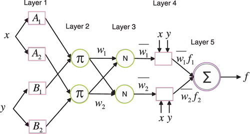
The first layer of the network belongs to the linguistic terms come from input parameters. These linguistic terms can be organized by Gaussian membership function. The below formulation expresses the Gaussian function (Ahangari, Moeinossadat, & Behnia, 2015): (9) $O_i^1=\beta \left(X\right)=\text{ex}{\text{p}}^{\left((-1/2)\left({\left(X-Z\right)}^2/{\sigma }^2\right)\right)}$(9) here, Z and σ indicate the Gaussian parameters.

The second layer belongs to the determination of weight terms based on rules: (10) $O_i^2=W_i={\beta }_{Ai}\left(X\right).{\beta }_{Bi}\left(X\right)$(10)

The third layer represents the process of determination of weight average values as following: (11) $O_i^3=\frac{W_i}{{\sum }^{W_i}}$(11)

In the fourth layer, a function in terms of average weight values is constructed as follows: (12) $O_i^4=\overline{W_i}{f}_i=\overline{W_i}\left(m_i{X}_1+n_i{X}_2+r_i\right)$(12)

Here, m, n, and r represent the resulting indexes.

In the last layer, the summation of previous layer outputs is determined such as the following: (13) $O_i^5=Y=\sum _i\overline{W_i}{f}_i=\overline{W_1}{f}_1+\overline{W_2}{f}_2=\frac{{\sum }^{W_i}{f}_i}{{\sum }^{W_i}}$(13)

3.3. Overview of PSO algorithm

Particle swarm optimization which was created based on existing populations in nature such as birds is known as one of the popular stochastic optimization methods. In this optimization algorithm, the promotion of initial population is optimization process; particles are known as the solutions and a swarm is a group of particles (Castillo, 2012; Eberhart & Kennedy, 1995; Onwunalu & Durlofsky, 2010; Panigrahi, Shi, & Lim, 2011).

In this algorithm, the particle velocity V_i(t) is updated by the following equation: (14) $\begin{array}{rl}{v}_{id}\left(t+1\right)& =w{v}_{id}\left(t\right)+c_1{r}_1\left(p_{\text{best},\text{id}}\left(t\right)-X_{iid}\left(t\right)\right)\\ & +c_2{r}_2\left(g_{\text{best},\text{d}}\left(t\right)-X_{id}\left(t\right)\right),\\ & d=1,2,\dots ,D\end{array}$(14) p_best,id and g_best,id are known as the best position of particle and global position c, r and w denote the learning rate,random number and inertia weight. Also the position of particle can be determined as following (Chiou, Tsai, & Liu, 2012; Eberhart & Kennedy, 1995; Shi & Eberhart, 1998): (15) $X_{id}\left(t+1\right)=X_{id}\left(t\right)+v_{id}\left(t+1\right)d=1,2,\dots ,D$(15)

4. Results and discussions

4.1. Data preparation

Efficiency and consistency of any developed algorithm is extremely function of utilized real data points which need to be precise and easily accessible in order to carry out the algorithm (Baghban, Bahadori, et al., 2017; Baghban, Mohammadi, et al., 2017). A general model was evolved in the present work utilizing 1109 actual data points from reliable papers for 29 various fluids (Chen, Xie, Li, & Yu, 2008; Choi, Zhang, Yu, Lockwood, & Grulke, 2001; Chon, Kihm, Lee, & Choi, 2005; Das, Putra, Thiesen, & Roetzel, 2003; Eastman, Choi, Li, Yu, & Thompson, 2001; Fedele, Colla, & Bobbo, 2012; Godson, Lal, & Wongwises, 2010; Godson, Raja, Lal, & Wongwises, 2010; Halelfadl, Maré, & Estellé, 2014; Hwang et al., 2006; Jiang, Ding, & Peng, 2009; Jiang et al., 2014; Kazemi-Beydokhti, Heris, Moghadam, Shariati-Niasar, & Hamidi, 2014; Khedkar, Sonawane, & Wasewar, 2012; Kim, Choi, & Kim, 2007; Lee, Choi, Li, & Eastman, 1999; Mintsa, Roy, Nguyen, & Doucet, 2009; Moghadassi, Hosseini, & Henneke, 2010; Mondragón, Segarra, Martínez-Cuenca, Juliá, & Jarque, 2013; Murshed, 2012; Murshed et al., 2008; Nan, Shi, & Lin, 2003; Pastoriza-Gallego, Lugo, Cabaleiro, Legido, & Piñeiro, 2014; Patel, Sundararajan, & Das, 2010; Rashmi, Khalid, Ismail, Saidur, & Rashid, 2015; Thang, Khoi, & Minh, 2015; Zerradi, Ouaskit, Dezairi, Loulijat, & Mizani, 2014). The details of used nanofluids as ranges of void fraction, ranges of particle diameter, ranges of temperature and their references were reported in Table S1. On the other hand, Table S2 summarized the thermal conductivity of particle and base fluid. The second step after preparation of data is choosing the input and output parameters for the estimating algorithms. The input parameters of proposed LSSVM and ANFIS models were the base fluid thermal conductivity (W/mK), the nanoparticle thermal conductivity (W/mK), temperature (K), void fraction (v) and particle diameter (nm). Also for the outputs of algorithms, the nanofluids thermal conductivity was assumed. The collected dataset has been divided into the testing and training data subsets to prepare and evaluate the algorithms. A quarter of total dataset was selected randomly as a testing dataset and other 75% of data points was applied for the training of the LSSVM and ANFIS approaches.

4.2. Model development and evaluation

Due to the fewer number of tuning terms and high-speed computations of radial basis function (RBF) kernel respect to other functions, the aforementioned function was selected as a useful kernel function in compliance with published papers. In the LSSVM approach combined with radial basis function, a remarkable problem is to find two terms (i.e. $\gamma$ and σ²) as mentioned before. These two tuning parameters have a dominant application in order to reach a high-performance LSSVM approach with an acceptable degree of globalizations and approximations, where σ² refers to the kernel sample variance $\gamma$ expresses the regularization term.

The current paper applies the particle swarm optimization (PSO) approach for the calculation of optimal values of $\gamma$ and σ². The fundamental of the optimization approach is to obtain less value of a cost function (i.e. mean absolute relative error for the testing phase in this study). The optimization process has been continued some iterations as efforts to reach an accesable global best condition based on the presented fitness function. The suggested ANFIS model includes 10 clusters and 120 membership function parameters, which were determined by the optimization algorithm.

Figures 2 and 3 illustrates a diagrams of PSO-LSSVM and PSO-ANFIS models used in the present paper. Moreover, the characterizations of proposed models have been presented in Table 1. This table contains the number of utilized data in different steps of proposing algorithms, tuning parameters, number of iteration to reach the criteria and kernel function type.

Figure 2. Schematic diagram of proposed PSO-LSSVM model.

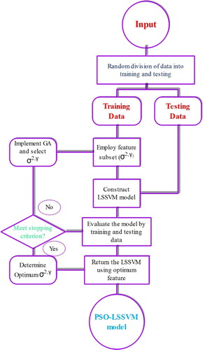
Figure 3. Schematic diagram of proposed PSO-ANFIS model.

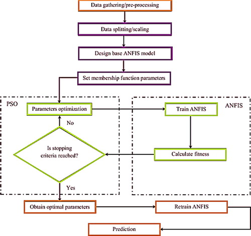
Table 1. Details of trained LSSVM and ANFIS algorithms.

Type	Comment/ value	Type	Comment/ value
LSSVM		ANFIS
Kernel function	RBF	Membership function	Gaussian
σ^2	0.4326	No. of membership function parameters	120
ϒ	10626.6529	No. of clusters	10
Optimization method	PSO	Optimization method	PSO
Number of data utilized for training	961	Number of data utilized for training	961
Number of data utilized for testing	320	Number of data utilized for testing	320
Population size	110	Population size	80
Maximum Iteration	1500	Maximum Iteration	1000
C1	1	C1	1
C2	2	C2	2

The approximations by the suggested LSSVM and ANFIS models were assessed by using different methods such as the graphical and statistical confirmations. The cross diagrams of suggested models which are made through depicting predicted against measured values were shown in Figures 4 and 5 for LSSVM and ANFIS, respectively. Based on observations obtained from this figure, a satisfactory agreement exists between estimated and measured nanofluid thermal conductivity values for ANFIS and LSSVM algorithms due to the close distribution of data points around the identity line. As it is obvious in this figure the predicted and real thermal conductivity of nanofluid cover each other in an appropriate manner for both proposed models.

Figure 4. Regression plots between experimental and estimated thermal conductivity by LSSVM for: (a) training data, (b) testing data (c) total data.

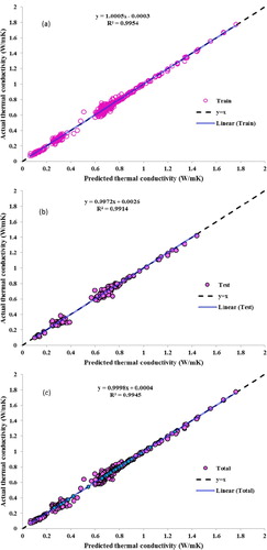
Figure 5. Regression plots between experimental and estimated thermal conductivity by ANFIS for: (a) training data, (b) testing data (c) total data.

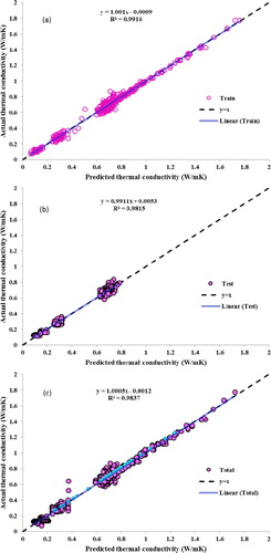
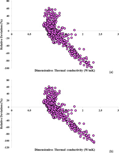
Figure 6 illustrates the relative errors of predicted thermal conductivity of nanofluid and measured points for both models. As shown, the horizontal axis representes the measured thermal conductivity of nanofluid and the vertical axis denotes the absolute error percent. The outcomes of this figure express that the obtained error values by the LSSVM and ANFIS algorithms range mostly of 5 to −5 percentage which proves the remarkable performance capacity of suggested models. In order to indicate deviations in a better way, relative deviations of two developed models are shown in Figure 7 versus dimensionless thermal conductivity which is a ratio of thermal conductivity of mixture and base fluid. As shown, both models have relatively similar deviations.

Figure 6. Absolute deviation of suggested models: (a) LSSVM, (b) ANFIS.

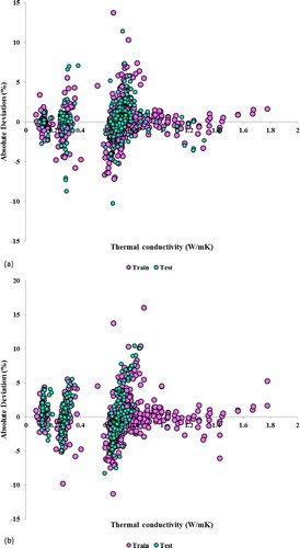
Figure 7. Relative deviation of suggested models: (a) LSSVM, (b) ANFIS.

Beside these graphical assessments, some popular statistical approaches were applied base on the below equations in order to confirm the satisfactory utilization of our suggested LSSVM and ANFIS models.

• The coefficient of determination (R²) (16) $R^2=1-\frac{{\sum }_{i=1}^N{\left(y_{\text{Pred}}\left(i\right)-y_{\text{Exp}}\left(i\right)\right)}^2}{{\sum }_{i=1}^N{\left(y_{\text{Pred}}\left(i\right)-{\overline{y}}_{\text{Exp}}\right)}^2}$(16)

• average absolute relative deviation (17) $\text{\%AARD}=\frac{100}{N}\sum _{i=1}^N\frac{\left(y_{\text{Pred}}\left(i\right)-y_{\text{Exp}}\left(i\right)\right)}{y_{\text{Exp}}\left(i\right)}$(17)

• Root Mean squared error (RMSE) (18) $\text{RMSE}={\left(\frac{{\sum }_{i=1}^N{\left(y_{\text{Pred}}\left(i\right)-y_{\text{Exp}}\left(i\right)\right)}^2}{N}\right)}^{0.5}$(18)

• Standard deviations (STD) (19) $\text{STD}=\sum _{i=1}^N{\left(\frac{{\left(y_{\text{Pred}}\left(i\right)-{\overline{y}}_{\text{Exp}}\left(i\right)\right)}^2}{N}\right)}^{0.5}$(19)

The abovementioned statistical analyses were summarized in Table 2 for the LSSVM and ANFIS models at three phases of train, test and overall.

Table 2. Statistical analyses obtained from the models.

	LSSVM			ANFIS
Analysis	Total	Training	Testing	Total	Training	Testing
R^2	0.994	0.995	0.991	0.984	0.992	0.983
AARD (%)	2.621	2.462	3.098	5.736	3.278	6.057
MSE	0.001	0.001	0.001	0.001	0.001	0.001
RMSE	0.02	0.019	0.023	0.034	0.025	0.032
STD	0.015	0.014	0.017	0.024	0.019	0.020

The present table indicates that the LSSVM and ANFIS models display reasonably low values of RMSE, AARD, and STD and high values of R-squared. The determined R² for LSSVM and ANFIS are 0.994 and 0.984 respectively. Also, the RMSE values for LSSVM and ANFIS were determined as 0.02 and 0.034 respectively. These analyses confirm the consistency and applicability of suggested models in order to predict the thermal conductivity of nanofluids. Also, these analyses show that the LSSVM algorithm has better performance respect to the ANFIS algorithm.

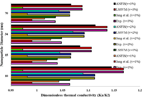
Lots of comparisons were implemented between the results of suggested ANFIS and LSSVM models and other published correlations. For Al₂O₃-water nanofluid has d_p= 38.4 nm at temperature of 324 K, the predicted dimensionless thermal conductivities by Mintsa, Nan, Murshed, Yu-Choi, Xie, and Chon et al. correlations have been compared with suggested LSSVM and ANFIS models in Figure 8 (Chon et al., 2005; Mintsa et al., 2009; Murshed et al., 2008; Nan, Birringer, Clarke, & Gleiter, 1997; Xie et al., 2005; Yu & Choi, 2003). As can be seen, as the nanoparticle volume fraction increases the dimensionless thermal conductivity also increases. Four other correlations such as the Godson, Wasp, Timofeeva, and Hamilton Correlations have been applied in order to compare with suggested LSSVM and ANFIS models for predicting Ag-water nanofluid dimensionless thermal conductivity with d_p= 63 nm and temperature of 343 K (Godson, Raja et al., 2010; Hamilton & Crosser, 1962; Timofeeva, Moravek, & Singh, 2011; Wasp, Kenny, & Gandhi, 1977). This comparison was shown in Figure 9 and results obtained from the present model have great accuracy with corresponding experimental dimensionless thermal conductivity. Thang correlation has been compared with our suggested models to predict carbon nanotube-water nanofluid dimensionless thermal conductivity as shown in Figure 10 (Thang et al., 2015). Furthermore, another comparison of the mentioned correlation and predicting models at a temperature of 296.15 K for carbon nanotube-water nanofluid has been indicated in Figure 11. These above two figure can indicate a greatly satisfactory prediction of LSSVM model than Thang et al. correlation. Moreover, another comparison was carried out in Figure 12 between the outcomes of suggested LSSVM and ANFIS models and four other correlations namely the Corcione, Vajjha, Patel and Azmi correlations for determining the CuO-water nanofluid dimensionless thermal conductivity that has a particle diameter of 24 nm at T = 298.15 K (Azmi, Sharma, Mamat, Alias, & Misnon, 2012; Corcione, 2011; Vajjha & Das, 2009). Moreover, for TiO₂-EG nanofluid at 298.15 K, the predicted dimensionless thermal conductivity by Jang’s correlation and ANFIS and LSSVM models at different nanoparticle size and volume void fraction has been illustrated in Figure 13 (Jang & Choi, 2004).

Figure 8. Comparison of LSSVM and ANFIS models with different models to estimate dimensionless thermal conductivity of Al₂O₃-water nanofluid.

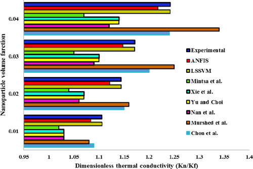
Figure 9. Comparison of LSSVM and ANFIS models with different models to estimate dimensionless thermal conductivity of Ag-water nanofluid.

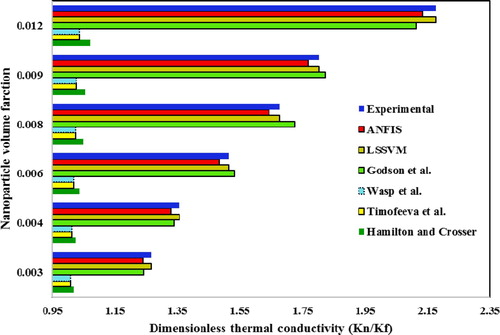
Figure 10. Comparison of LSSVM and ANFIS models with Thang et al. model to estimate dimensionless thermal conductivity of CNT-water nanofluid at different temperatures.

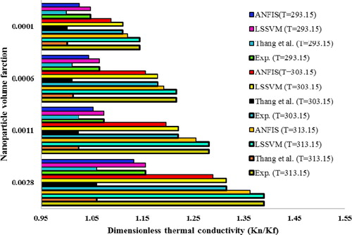
Figure 11. Comparison of LSSVM and ANFIS models with Thang et al. model to estimate dimensionless thermal conductivity of CNT-water nanofluid for different particle sizes.

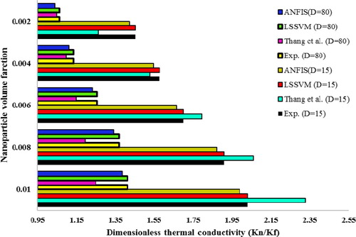
Figure 12. Comparison of LSSVM and ANFIS models with different models to estimate dimensionless thermal conductivity of CuO-water nanofluid.

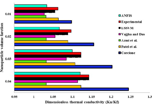
Figure 13. Comparison of LSSVM and ANFIS models with Jang et al. models to estimate dimensionless thermal conductivity of TiO₂-EG nanofluid for different volume void fractions and size particles.

As can be concluded, artificial intelligence based approaches can satisfactory applications in complicated cases such as nanofluid systems. Both developed models have great accuracy in order to estimate the thermal conductivity of nanofluids compared to other previously developed models. It is worth mentioning that the great advantage of these techniques is their simple application (as you can see the supplementary content) beside their accuracy.

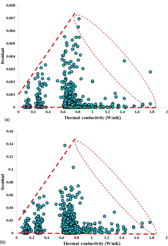
The experimental data which are used in the comparisons in Figures 8–13 can be identified with blue color in the cross plot. As can be observed from all the above comparisons, the suggested LSSVM have the satisfactory predictive capacity to forecast the dimensionless thermal conductivity of nanofluids. The residual plot which shows a difference in residual variance versus experimental thermal conductivity was shown in Figure 14 for both models. Heteroscedasticity produces a distinctive fan or cone shape in residual plots. As can be seen, this pattern has a cone-shape and it is shown the errors are normally distributed.

Figure 14. Residual plots for: (a) ANFIS (b) LSSVM models.

4.3. Outlier detection and sensitivity analysis

The measured data applied in the computational investigation can highly influence the predictive ability of our proposed algorithms (Rousseeuw & Leroy, 2005). As there is a various source of measurement errors of actual datasets in the literature, identification of outlier and suspected data for utilized experimental data points can indicate greatly bad experimental data points.

William’s plot as a graphical illustration can help us to identify accurately and suspected data points. This figure has been depicted in Figure 15 for LSSVM and ANFIS algorithm models to detect outliers.

Figure 15. Outlier analysis of the suggested (a) LSSVM and (b) ANFIS models.

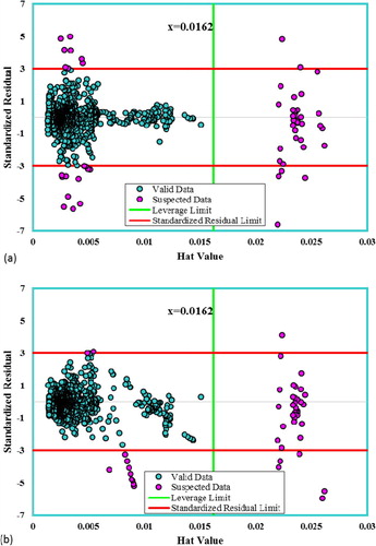
Besides, the leverage boundary is defined base on the green line and the experimental data which their hat values (H) are more than the criterion value H* are known as outliers. H and H* can be determined as following: (20) $\begin{array}{rl}H& =X(X^{T}X{)}^{-1}{X}^T\end{array}$(20) (21) $\begin{array}{rl}{H}^{\ast }& =3\left(n+1\right)/m\end{array}$(21) where X represents as the m×n matrix that n and m denote the model indexes number and number of samples (Mohammadi, Gharagheizi, Eslamimanesh, & Richon, 2012). The standardized residual values have the values of −3 and + 3 are shown by red color is shown in Figure 15 so the accurate experimental data are also located inside of the defined boundaries.

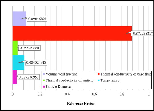
One of the popular statistical approaches is Sensitivity analysis to illustrate the relationship between output and inputs. The impact of input parameters on the target parameter is identified by the relevancy factor (r) and in the current work, we are going find out the effect inputs on thermal conductivity of nanofluids. The relevancy factor can be determined as below: (22) $r=\frac{{\sum }_{i=1}^n(X_{k,i}-\overline{X_k})\left(Y_i-\overline{Y}\right)}{\sqrt{{\sum }_{i=1}^n{(X_{k,i}-\overline{X_k})}^2{\sum }_{i=1}^n(Y_i-{\overline{Y)}}^2}}$(22) where $Y_i$,$\overline{Y}$,$X_{k,i}$ and $\overline{X_k}$ are the ‘i’^th output, output average, k^th of input and average of input (Hosseinzadeh & Hemmati-Sarapardeh, 2014; Razavi, Bemani, Baghban, Mohammadi, & Habibzadeh, 2019). The aforementioned index is varied between −1 and + 1 and as this term has the higher value is for a specific input variable, it can be understood that this input variable has much influence on the output. A negative value indicates a decreasing effect and Positive value has an increasing effect (Hosseinzadeh & Hemmati-Sarapardeh, 2014).

As it is obvious in Figure 16, the volume void fraction, thermal the conductivity of the base fluid and temperature has a straight relationship with nanofluid thermal conductivity values. Due to determined r values for different parameters, the particle diameter is the weakest parameter on target parameter determination and the most effective parameter is thermal conductivity of the base fluid.

Figure 16. Sensitivity analysis of parameters used for developing model.

5. Conclusions

In the current paper, different statistical and graphical analyses are carried out to find a high-performance method for estimation of thermal conductivity of nanofluids. This investigation was concluded to the following results:

• In order to show the acceptable performance of LSSVM and ANFIS algorithms, a comprehensive dataset from existing experimental studies in literature has been gathered.

• The LSSVM and ANFIS algorithms reach the best performance structure by the employment of the PSO algorithm. Furthermore, a high degree of accuracy was observed in the prediction of the thermal conductivity of different nanofluids by LSSVM and ANFIS algorithms.

• In the purpose of illustrating the predictive ability of proposed models, the LSSVM and ANFIS algorithms have been compared with 15 different correlation based methods for estimation of nanofluids thermal conductivity. The comparisons expressed the amazing performance of LSSVM algorithm.

• The current study has proposed two accurate methods which can be used as simple and user friend software in different projects.

• In the current work, a great mathematical analysis has been used to improve the accuracy of predictive models by separating suspected experimental data.

• A sensitivity analysis has been used to show the impact of different parameters on the thermal conductivity of nanofluids. This analysis expresses that thermal conductivity of base fluid is the most effective parameter in the determination of thermal conductivity of nanofluids. Also, the particle diameter is the least effective parameter in this process.

According to the aforementioned conclusions, the current work can be a comprehensive and helpful study about the heat transfer process in nanofluids which makes this work valuable for engineers and researchers. As a future suggestion, the current results can be compared with other modeling approaches such as numerical modeling and artificial intelligence based approaches (Genetic programing, committee machine intelligence system, and artificial neural network).

Disclosure statement

No potential conflict of interest was reported by the authors.

ORCID

Alireza Baghban http://orcid.org/0000-0002-7224-4704

Appendix: The authors' model

In this work, the LSSVM algorithm was prepared in form of a graphical user interface (GUI). This supplementary contains an exe file that requires Matlab software version 2012 (64bit). This GUI has three input parameters (volume void fraction diameter and temperature) should be entered and then selecting one of the nanofluids and then by choosing to the calculate button, it will obtain the thermal conductivity of nanofluid.

References

- Abdi-Khanghah, M., Bemani, A., Naserzadeh, Z., & Zhang, Z. (2018). Prediction of solubility of N-alkanes in supercritical CO2 using RBF-ANN and MLP-ANN. Journal of CO2 Utilization, 25, 108–119.
- Afshar, M., Gholami, A., & Asoodeh, M. (2014). Genetic optimization of neural network and fuzzy logic for oil bubble point pressure modeling. Korean Journal of Chemical Engineering, 31(3), 496–502.
- Ahangari, K., Moeinossadat, S. R., & Behnia, D. (2015). Estimation of tunnelling-induced settlement by modern intelligent methods. Soils and Foundations, 55(4), 737–748.
- Ahmadi, M. H., Ghahremannezhad, A., Chau, K.-W., Seifaddini, P., Ramezannezhad, M., & Ghasempour, R. (2019). Development of simple-to-use predictive models to determine thermal properties of Fe2O3/water-ethylene glycol nanofluid. Computation, 7(1), 18.
- Ahmadi, M. H., Mohseni-Gharyehsafa, B., Farzaneh-Gord, M., Jilte, R. D., Kumar, R., & Chau, K.-w. (2019). Applicability of connectionist methods to predict dynamic viscosity of silver/water nanofluid by using ANN-MLP, MARS and MPR algorithms. Engineering Applications of Computational Fluid Mechanics, 13(1), 220–228.
- Ahmadi, M. H., Sadeghzadeh, M., Raffiee, A. H., & Chau, K.-w. (2019). Applying GMDH neural network to estimate the thermal resistance and thermal conductivity of pulsating heat pipes. Engineering Applications of Computational Fluid Mechanics, 13(1), 327–336.
- Ali Ghorbani, M., Kazempour, R., Chau, K.-W., Shamshirband, S., & Taherei Ghazvinei, P. (2018). Forecasting pan evaporation with an integrated artificial neural network quantum-behaved particle swarm optimization model: A case study in Talesh, Northern Iran. Engineering Applications of Computational Fluid Mechanics, 12(1), 724–737.
- Ariana, M., Vaferi, B., & Karimi, G. (2015). Prediction of thermal conductivity of alumina water-based nanofluids by artificial neural networks. Powder Technology, 278, 1–10.
- Atashrouz, S., Pazuki, G., & Alimoradi, Y. (2014). Estimation of the viscosity of nine nanofluids using a hybrid GMDH-type neural network system. Fluid Phase Equilibria, 372, 43–48.
- Azmi, W., Sharma, K., Mamat, R., Alias, A., & Misnon, I. I. (2012). Correlations for thermal conductivity and viscosity of water based nanofluids. IOP Conference Series: Materials Science and Engineering.
- Baghban, A., Ahmadi, M. A., Pouladi, B., & Amanna, B. (2015). Phase equilibrium modeling of semi-clathrate hydrates of seven commonly gases in the presence of TBAB ionic liquid promoter based on a low parameter connectionist technique. The Journal of Supercritical Fluids, 101, 184–192.
- Baghban, A., Ahmadi, M. A., & Shahraki, B. H. (2015). Prediction carbon dioxide solubility in presence of various ionic liquids using computational intelligence approaches. The Journal of Supercritical Fluids, 98, 50–64.
- Baghban, A., Bahadori, A., Mohammadi, A. H., & Behbahaninia, A. (2017). Prediction of CO2 loading capacities of aqueous solutions of absorbents using different computational schemes. International Journal of Greenhouse Gas Control, 57, 143–161.
- Baghban, A., Bahadori, M., Rozyn, J., Lee, M., Abbas, A., Bahadori, A., & Rahimali, A. (2016). Estimation of air dew point temperature using computational intelligence schemes. Applied Thermal Engineering, 93, 1043–1052.
- Baghban, A., Mohammadi, A. H., & Taleghani, M. S. (2017). Rigorous modeling of CO2 equilibrium absorption in ionic liquids. International Journal of Greenhouse Gas Control, 58, 19–41. doi: 10.1016/j.ijggc.2016.12.009
- Bahadori, A., Baghban, A., Bahadori, M., Lee, M., Ahmad, Z., Zare, M., & Abdollahi, E. (2016). Computational intelligent strategies to predict energy conservation benefits in excess air controlled gas-fired systems. Applied Thermal Engineering, 102, 432–446. doi: 10.1016/j.applthermaleng.2016.04.005
- Bruggeman, V. D. (1935). Berechnung verschiedener physikalischer Konstanten von heterogenen Substanzen. I. Dielektrizitätskonstanten und Leitfähigkeiten der Mischkörper aus isotropen Substanzen. Annalen der Physik, 416(7), 636–664.
- Castillo, O. (2012). Introduction to type-2 fuzzy logic control. In O. Castillo (Ed.), Type-2 fuzzy logic in intelligent control applications (pp. 3–5). Berlin: Springer.
- Chau, K.-w. (2017). Use of meta-heuristic techniques in rainfall-runoff modelling. Water, 9(3), 186–191. doi: 10.3390/w9030186
- Chein, R., & Chuang, J. (2007). Experimental microchannel heat sink performance studies using nanofluids. International Journal of Thermal Sciences, 46(1), 57–66.
- Chen, L., Xie, H., Li, Y., & Yu, W. (2008). Nanofluids containing carbon nanotubes treated by mechanochemical reaction. Thermochimica Acta, 477(1), 21–24.
- Cheng, C. T., & Chau, K.-W. (2002). Three-person multi-objective conflict decision in reservoir flood control. European Journal of Operational Research, 142(3), 625–631.
- Chiou, J.-S., Tsai, S.-H., & Liu, M.-T. (2012). A PSO-based adaptive fuzzy PID-controllers. Simulation Modelling Practice and Theory, 26, 49–59.
- Choi, S., Zhang, Z., Yu, W., Lockwood, F., & Grulke, E. (2001). Anomalous thermal conductivity enhancement in nanotube suspensions. Applied Physics Letters, 79(14), 2252–2254.
- Chol, S. (1995). Enhancing thermal conductivity of fluids with nanoparticles. ASME-Publications-Fed, 231, 99–106.
- Chon, C. H., Kihm, K. D., Lee, S. P., & Choi, S. U. (2005). Empirical correlation finding the role of temperature and particle size for nanofluid (Al2O3) thermal conductivity enhancement. Applied Physics Letters, 87(15), 153107.
- Corcione, M. (2011). Empirical correlating equations for predicting the effective thermal conductivity and dynamic viscosity of nanofluids. Energy Conversion and Management, 52(1), 789–793.
- Das, S. K., Putra, N., Thiesen, P., & Roetzel, W. (2003). Temperature dependence of thermal conductivity enhancement for nanofluids. Journal of Heat Transfer, 125(4), 567–574.
- Eastman, J. A., Choi, S., Li, S., Yu, W., & Thompson, L. (2001). Anomalously increased effective thermal conductivities of ethylene glycol-based nanofluids containing copper nanoparticles. Applied Physics Letters, 78(6), 718–720.
- Eberhart, R., & Kennedy, J. (1995). A new optimizer using particle swarm theory. Proceedings of the Sixth International Symposium on Micro Machine and Human Science, MHS'95.
- Ebrahimnia-Bajestan, E., Moghadam, M. C., Niazmand, H., Daungthongsuk, W., & Wongwises, S. (2016). Experimental and numerical investigation of nanofluids heat transfer characteristics for application in solar heat exchangers. International Journal of Heat and Mass Transfer, 92, 1041–1052.
- Eiamsa-ard, S., & Wongcharee, K. (2018). Experimental study of TiO2-water nanofluid flow in corrugated tubes mounted with semi-circular wing tapes. Heat Transfer Engineering, 39(1), 1–14.
- Esfe, M. H., Afrand, M., Yan, W.-M., & Akbari, M. (2015). Applicability of artificial neural network and nonlinear regression to predict thermal conductivity modeling of Al2O3–water nanofluids using experimental data. International Communications in Heat and Mass Transfer, 66, 246–249.
- Evans, W., Prasher, R., Fish, J., Meakin, P., Phelan, P., & Keblinski, P. (2008). Effect of aggregation and interfacial thermal resistance on thermal conductivity of nanocomposites and colloidal nanofluids. International Journal of Heat and Mass Transfer, 51(5), 1431–1438.
- Fedele, L., Colla, L., & Bobbo, S. (2012). Viscosity and thermal conductivity measurements of water-based nanofluids containing titanium oxide nanoparticles. International Journal of Refrigeration, 35(5), 1359–1366.
- Ghalambaz, M., Sheremet, M. A., & Pop, I. (2015). Free convection in a parallelogrammic porous cavity filled with a nanofluid using Tiwari and Das.
- Godson, L., Lal, D. M., & Wongwises, S. (2010). Measurement of thermo physical properties of metallic nanofluids for high temperature applications. Nanoscale and Microscale Thermophysical Engineering, 14(3), 152–173.
- Godson, L., Raja, B., Lal, D. M., & Wongwises, S. (2010). Experimental investigation on the thermal conductivity and viscosity of silver-deionized water nanofluid. Experimental Heat Transfer, 23(4), 317–332.
- Guo, Z., & Bai, G. (2009). Application of least squares support vector machine for regression to reliability analysis. Chinese Journal of Aeronautics, 22(2), 160–166.
- Halelfadl, S., Maré, T., & Estellé, P. (2014). Efficiency of carbon nanotubes water based nanofluids as coolants. Experimental Thermal and Fluid Science, 53, 104–110.
- Hamilton, R., & Crosser, O. (1962). Thermal conductivity of heterogeneous two-component systems. Industrial & Engineering Chemistry Fundamentals, 1(3), 187–191.
- Hojjat, M., Etemad, S. G., Bagheri, R., & Thibault, J. (2011). Thermal conductivity of non-Newtonian nanofluids: Experimental data and modeling using neural network. International Journal of Heat and Mass Transfer, 54(5), 1017–1023.
- Hosseinzadeh, M., & Hemmati-Sarapardeh, A. (2014). Toward a predictive model for estimating viscosity of ternary mixtures containing ionic liquids. Journal of Molecular Liquids, 200, 340–348.
- Hwang, Y., Ahn, Y., Shin, H., Lee, C., Kim, G., Park, H., & Lee, J. (2006). Investigation on characteristics of thermal conductivity enhancement of nanofluids. Current Applied Physics, 6(6), 1068–1071.
- Jang, J. S. R., Sun, C. T., & Mizutani, E. (1997). Neuro-fuzzy and soft computing-a computational approach to learning and machine intelligence. IEEE Transactions on Automatic Control, 42(10), 1482–1484.
- Jang, S. P., & Choi, S. U. (2004). Role of Brownian motion in the enhanced thermal conductivity of nanofluids. Applied Physics Letters, 84(21), 4316–4318.
- Jiang, H., Li, H., Zan, C., Wang, F., Yang, Q., & Shi, L. (2014). Temperature dependence of the stability and thermal conductivity of an oil-based nanofluid. Thermochimica Acta, 579, 27–30.
- Jiang, W., Ding, G., & Peng, H. (2009). Measurement and model on thermal conductivities of carbon nanotube nanorefrigerants. International Journal of Thermal Sciences, 48(6), 1108–1115.
- Karimi, H., & Yousefi, F. (2012). Application of artificial neural network–genetic algorithm (ANN–GA) to correlation of density in nanofluids. Fluid Phase Equilibria, 336, 79–83.
- Karimi, H., Yousefi, F., & Rahimi, M. R. (2011). Correlation of viscosity in nanofluids using genetic algorithm-neural network (GA-NN). Heat and Mass Transfer, 47(11), 1417–1425.
- Karkevandi-Talkhooncheh, A., Hajirezaie, S., Hemmati-Sarapardeh, A., Husein, M. M., Karan, K., & Sharifi, M. (2017). Application of adaptive neuro fuzzy interface system optimized with evolutionary algorithms for modeling CO2-crude oil minimum miscibility pressure. Fuel, 205, 34–45.
- Kazemi-Beydokhti, A., Heris, S. Z., Moghadam, N., Shariati-Niasar, M., & Hamidi, A. (2014). Experimental investigation of parameters affecting nanofluid effective thermal conductivity. Chemical Engineering Communications, 201(5), 593–611.
- Keblinski, P., Phillpot, S., Choi, S., & Eastman, J. (2002). Mechanisms of heat flow in suspensions of nano-sized particles (nanofluids). International Journal of Heat and Mass Transfer, 45(4), 855–863.
- Khedkar, R. S., Sonawane, S. S., & Wasewar, K. L. (2012). Influence of CuO nanoparticles in enhancing the thermal conductivity of water and monoethylene glycol based nanofluids. International Communications in Heat and Mass Transfer, 39(5), 665–669.
- Kim, S. H., Choi, S. R., & Kim, D. (2007). Thermal conductivity of metal-oxide nanofluids: Particle size dependence and effect of laser irradiation. Journal of Heat Transfer, 129(3), 298–307.
- Kleinstreuer, C., & Feng, Y. (2011). Experimental and theoretical studies of nanofluid thermal conductivity enhancement: A review. Nanoscale Research Letters, 6(1), 1–13.
- Koo, J., & Kleinstreuer, C. (2004). A new thermal conductivity model for nanofluids. Journal of Nanoparticle Research, 6(6), 577–588.
- Lee, J.-H., Lee, S.-H., Choi, C., Jang, S., & Choi, S. (2011). A review of thermal conductivity data, mechanisms and models for nanofluids. International Journal of Micro-Nano Scale Transport, 4, 269–322.
- Lee, S., Choi, S.-S., Li, S., & Eastman, J. (1999). Measuring thermal conductivity of fluids containing oxide nanoparticles. Journal of Heat Transfer, 121(2), 280–289.
- Leong, K., Yang, C., & Murshed, S. (2006). A model for the thermal conductivity of nanofluids–the effect of interfacial layer. Journal of Nanoparticle Research, 8(2), 245–254.
- Longo, G. A., Zilio, C., Ceseracciu, E., & Reggiani, M. (2012). Application of artificial neural network (ANN) for the prediction of thermal conductivity of oxide–water nanofluids. Nano Energy, 1(2), 290–296.
- Maxwell, J. (1873). Electricity and magnetism. Oxford: Clarendon Press.
- Maxwell, J. C. (1881). A treatise on electricity and magnetism. Oxford: Clarendon Press.
- Mazumdar, A., Spencer, S. J., Hobart, C., Kuehl, M., Brunson, G., Coleman, N., & Buerger, S. P. (2016). Improving robotic actuator torque density and efficiency through enhanced heat transfer. ASME 2016 Dynamic Systems and Control Conference.
- Meybodi, M. K., Naseri, S., Shokrollahi, A., & Daryasafar, A. (2015). Prediction of viscosity of water-based Al2O3, TiO2, SiO2, and CuO nanofluids using a reliable approach. Chemometrics and Intelligent Laboratory Systems, 149, 60–69.
- Mintsa, H. A., Roy, G., Nguyen, C. T., & Doucet, D. (2009). New temperature dependent thermal conductivity data for water-based nanofluids. International Journal of Thermal Sciences, 48(2), 363–371.
- Moazenzadeh, R., Mohammadi, B., Shamshirband, S., & Chau, K.-w. (2018). Coupling a firefly algorithm with support vector regression to predict evaporation in northern Iran. Engineering Applications of Computational Fluid Mechanics, 12(1), 584–597.
- Moghadassi, A., Hosseini, S. M., & Henneke, D. E. (2010). Effect of CuO nanoparticles in enhancing the thermal conductivities of monoethylene glycol and paraffin fluids. Industrial & Engineering Chemistry Research, 49(4), 1900–1904.
- Mohammadi, A. H., Gharagheizi, F., Eslamimanesh, A., & Richon, D. (2012). Evaluation of experimental data for wax and diamondoids solubility in gaseous systems. Chemical Engineering Science, 81, 1–7.
- Mondragón, R., Segarra, C., Martínez-Cuenca, R., Juliá, J. E., & Jarque, J. C. (2013). Experimental characterization and modeling of thermophysical properties of nanofluids at high temperature conditions for heat transfer applications. Powder Technology, 249, 516–529.
- Murshed, S., Leong, K., & Yang, C. (2008). Investigations of thermal conductivity and viscosity of nanofluids. International Journal of Thermal Sciences, 47(5), 560–568.
- Murshed, S. S. (2012). Simultaneous measurement of thermal conductivity, thermal diffusivity, and specific heat of nanofluids. Heat Transfer Engineering, 33(8), 722–731.
- Nan, C.-W., Birringer, R., Clarke, D. R., & Gleiter, H. (1997). Effective thermal conductivity of particulate composites with interfacial thermal resistance. Journal of Applied Physics, 81(10), 6692–6699.
- Nan, C.-W., Shi, Z., & Lin, Y. (2003). A simple model for thermal conductivity of carbon nanotube-based composites. Chemical Physics Letters, 375(5), 666–669.
- Onwunalu, J. E., & Durlofsky, L. J. (2010). Application of a particle swarm optimization algorithm for determining optimum well location and type. Computational Geosciences, 14(1), 183–198.
- Panigrahi, B. K., Shi, Y., & Lim, M.-H. (2011). Handbook of swarm intelligence: Concepts, principles and applications. Berlin: Springer Science & Business Media.
- Papari, M. M., Yousefi, F., Moghadasi, J., Karimi, H., & Campo, A. (2011). Modeling thermal conductivity augmentation of nanofluids using diffusion neural networks. International Journal of Thermal Sciences, 50(1), 44–52.
- Pastoriza-Gallego, M., Lugo, L., Cabaleiro, D., Legido, J., & Piñeiro, M. (2014). Thermophysical profile of ethylene glycol-based ZnO nanofluids. The Journal of Chemical Thermodynamics, 73, 23–30.
- Patel, H. E., Sundararajan, T., & Das, S. K. (2010). An experimental investigation into the thermal conductivity enhancement in oxide and metallic nanofluids. Journal of Nanoparticle Research, 12(3), 1015–1031.
- Rashmi, W., Khalid, M., Ismail, A. F., Saidur, R., & Rashid, A. (2015). Experimental and numerical investigation of heat transfer in CNT nanofluids. Journal of Experimental Nanoscience, 10(7), 545–563.
- Razavi, R., Bemani, A., Baghban, A., Mohammadi, A. H., & Habibzadeh, S. (2019). An insight into the estimation of fatty acid methyl ester based biodiesel properties using a LSSVM model. Fuel, 243, 133–141.
- Rousseeuw, P. J., & Leroy, A. M. (2005). Robust regression and outlier detection. Hoboken, NJ: John Wiley & Sons.
- Sharifpur, M., Adio, S. A., & Meyer, J. P. (2015). Experimental investigation and model development for effective viscosity of Al2O3–glycerol nanofluids by using dimensional analysis and GMDH-NN methods. International Communications in Heat and Mass Transfer, 68, 208–219.
- Sheremet, M., Groşan, T., & Pop, I. (2015). Steady-state free convection in right-angle porous trapezoidal cavity filled by a nanofluid: Buongiorno’s mathematical model. European Journal of Mechanics-B/Fluids, 53, 241–250.
- Shi, Y., & Eberhart, R. (1998). A modified particle swarm optimizer. 1998 IEEE international conference on Evolutionary Computation Proceedings. IEEE World Congress on Computational Intelligence.
- Sohrabi, N., Masoumi, N., Behzadmehr, A., & Sarvari, S. (2010). A simple analytical model for calculating the effective thermal conductivity of nanofluids. Heat Transfer—Asian Research, 39(3), 141–150.
- Suykens, J. A., & Vandewalle, J. (1999). Least squares support vector machine classifiers. Neural Processing Letters, 9(3), 293–300.
- Suykens, J. A., & Vandewalle, J. (2000). Recurrent least squares support vector machines. IEEE Transactions on Circuits and Systems I: Fundamental Theory and Applications, 47(7), 1109–1114.
- Suykens, J. A., Van Gestel, T., & De Brabanter, J. (2002). Least squares support vector machines. London: World Scientific.
- Thang, B. H., Khoi, P. H., & Minh, P. N. (2015). A modified model for thermal conductivity of carbon nanotube-nanofluids. Physics of Fluids, 27(3), 032002.
- Timofeeva, E. V., Moravek, M. R., & Singh, D. (2011). Improving the heat transfer efficiency of synthetic oil with silica nanoparticles. Journal of Colloid and Interface Science, 364(1), 71–79.
- Tomlinson, H. L., Manning, W., Schaefer, W., & Record, T. (2016). Process for increasing the efficiency of heat removal from a Fischer-Tropsch slurry reactor: Google Patents.
- Vajjha, R. S., & Das, D. K. (2009). Experimental determination of thermal conductivity of three nanofluids and development of new correlations. International Journal of Heat and Mass Transfer, 52(21), 4675–4682.
- Vatani, A., Woodfield, P. L., & Dao, D. V. (2015). A survey of practical equations for prediction of effective thermal conductivity of spherical-particle nanofluids. Journal of Molecular Liquids, 211, 712–733.
- Wasp, E. J., Kenny, J. P., & Gandhi, R. L. (1977). Solid-liquid flow slurry pipeline transportation (Vol. 1, Series on bulk materials handling). Clausthal: Trans Tech Publications.
- Wen, D., Lin, G., Vafaei, S., & Zhang, K. (2009). Review of nanofluids for heat transfer applications. Particuology, 7(2), 141–150.
- Wu, C., & Chau, K. (2011). Rainfall–runoff modeling using artificial neural network coupled with singular spectrum analysis. Journal of Hydrology, 399(3–4), 394–409.
- Xie, H., Fujii, M., & Zhang, X. (2005). Effect of interfacial nanolayer on the effective thermal conductivity of nanoparticle-fluid mixture. International Journal of Heat and Mass Transfer, 48(14), 2926–2932.
- Xu, J., Yu, B., Zou, M., & Xu, P. (2006). A new model for heat conduction of nanofluids based on fractal distributions of nanoparticles. Journal of Physics D: Applied Physics, 39(20), 4486–4490.
- Yaseen, Z. M., Sulaiman, S. O., Deo, R. C., & Chau, K.-W. (2019). An enhanced extreme learning machine model for river flow forecasting: State-of-the-art, practical applications in water resource engineering area and future research direction. Journal of Hydrology, 569, 387–408.
- Yu, W., & Choi, S. (2003). The role of interfacial layers in the enhanced thermal conductivity of nanofluids: A renovated Maxwell model. Journal of Nanoparticle Research, 5(1–2), 167–171.
- Zalba, B., Marı´n, J. M., Cabeza, L. F., & Mehling, H. (2003). Review on thermal energy storage with phase change: Materials, heat transfer analysis and applications. Applied Thermal Engineering, 23(3), 251–283.
- Zeeshan, A., Shehzad, N., Ellahi, R., & Alamri, S. Z. (2017). Convective Poiseuille flow of Al2O3-EG nanofluid in a porous wavy channel with thermal radiation. Neural Computing and Applications, 30, 1–12.
- Zerradi, H., Ouaskit, S., Dezairi, A., Loulijat, H., & Mizani, S. (2014). New Nusselt number correlations to predict the thermal conductivity of nanofluids. Advanced Powder Technology, 25(3), 1124–1131.