Thin and sharp edges bodies-fluid interaction simulation using cut-cell immersed boundary method

Abstract

This study aims to develop an adaptive mesh refinement (AMR) algorithm combined with Cut-Cell IBM using two-stage pressure–velocity corrections for thin-object FSI problems. To achieve the objective of this study, the AMR-immersed boundary method (AMR-IBM) algorithm discretizes and solves the equations of motion for the flow that involves rigid thin structures boundary layer at the interface between the structure and the fluid. The body forces are computed in proportion to the fraction of the solid volume in the IBM fluid cells to incorporate fluid and solid motions into the boundary. The corrections of the velocity and pressure is determined by using a novel simplified marker and cell scheme. The new developed AMR-IBM algorithm is validated using a benchmark data of fluid past a cylinder and the results show that there is good agreement under laminar flow. Simulations are conducted for three test cases with the purpose of demonstration the accuracy of the AMR-IBM algorithm. The validation confirms the robustness of the new algorithms in simulating flow characteristics in the boundary layers of thin structures. The algorithm is performed on a staggered grid to simulate the fluid flow around thin object and determine the computational cost.

KEYWORDS:

• Cut-cell method
• adaptive mesh refinement
• pressure and velocity corrections
• thin objects and fluid structure

1. Introduction

Fluid Solid interaction (FSI) is the characterization of the variable relationship that occurs between flowing fluids and any solids. A solid structure may deform when subjected to forces generated by the movement of the solid inside the fluid. The investigation of such interactions is essential because it concerns various engineering designs and applications of any parts affected by fluid dynamics, such as aircraft wings, cruise ships, turbine blades, bridges, airbags or tent roofs. The numerical simulations of FSI have expanded their role in scientific research and engineering analysis (Ghalandari, Koohshahi, Shamshirband, & Chau, 2019). Accurate FSI simulations are regarded as cost-effective alternatives to scientific experiments in various industries.

In cases involving thin objects, the intricacies are difficult to capture, which leads to an inadequate understanding of the nature of the relationship between a solid and a surrounding fluid (Liang, Wei, Lu, & Qin, 2017; Mo, Lien, Zhang, & Cronin, 2018; Mou, He, Zhao, & Chau, 2017; Nasar, Rogers, Revell, Stansby, & Lind, 2019). These problems exist in many fields, such as chemistry (particulate flow), biology and engineering (Akbarian et al., 2018; Aldlemy, Rasani, Ya, & Ariffin, 2018; Gilmanov, Le, & Sotiropoulos, 2015; Lin, He, He, & Wang, 2018; Martínez-Ferrer, Qian, Ma, Causon, & Mingham, 2018; Ramezanizadeh, Alhuyi Nazari, Ahmadi, & Chau, 2019; Schott, Ager, & Wall, 2018; Tian, Dai, Luo, Doyle, & Rousseau, 2014). In environmental and biological studies, various fluid flows are involved in complex and thin bodies, such as the relative flow of fluid (air) around a leaf as it falls freely from its tree attachment, the flapping of a flag in the wind. Also, the elastic filament in a floating foams created by soap, or the solar sails in outer space navigating, the flow of fluid in two-stroke engines, the vibrations of the vocal folds, plasma and particles flow in the blood vessel and the relative flow of fluid past microorganisms (Kajishima & Taira, 2017; Rasani, Aldlemy, & Harun, 2017; Vadala-Roth, Rossi, & Griffith, 2018; Wang, Currao, et al., 2017).

In FSI problems, the flow characteristics within proximity of the surface of thin objects are determined by estimating the pressure and velocities of the flow in the boundary layer. Re-meshing is required whenever the thin object becomes displaced or deformed, which will increase the computational cost (Bourlet, Gurugubelli, & Jaiman, 2015; Fujisawa & Asada, 2016; Liu, Zhao, Hu, Goman, & Li, 2013; Yang, Yu, Krane, & Zhang, 2018). In this regard, fixed Cartesian mesh schemes are typically implemented for the discretization of the equations of fluid dynamics in order to estimate the flow characteristics of arbitrarily thin objects because of their simplicity and lower computational cost. In contrast, a rectangular mesh is computed in the immersed boundary method (IBM) and a few additional steps are implemented to identify the occupied cell fractions for arbitrarily shaped objects.

IBM was established by Charles Peskin (Goza & Colonius, 2017; Peskin, 1977, 1972; Peskin & McQueen, 1989), who worked on the FSI of fibers using numerical simulation. In Peskin’s approach, the heart valve is modeled such as a thin, viscoelastic solid threads with respect to both time and elasticity constraints (Lee & Lee, 2012; Mittal & Iaccarino, 2005). A number of studies presented by previous reviews for Immersed boundary method (IBM). It is considered into two main families: the continuous (or diffuse) and discrete (or sharp) methods. The diffused interface schemes via classical IB methods (Mori & Peskin, 2008; Peskin, 1972), direct forcing methods (Su, Lai, & Lin, 2007; Uhlmann, 2005), and penalization methods (Angot, Bruneau, & Fabrie, 1999; Kevlahan & Ghidaglia, 2001; Miao, Hendrickson, & Liu, 2017) can be categorized under cut-cell methods especially for sharp edges solid structure (Miao et al., 2017; Udaykumar, Mittal, Rampunggoon, & Khanna, 2001; Ye, Mittal, Udaykumar, & Shyy, 1999). In the IBM cut-cell methods (Kirkpatrick, Armfield, & Kent, 2003; Udaykumar et al., 2001), the governing equations are solved using finite difference (FD) as the original IBM and some cases for more accuracy finite volume approach (FV) replaced the FD methods. Bothe of the methods are accurate, satisfy the pressure decoupling constraint and are able to handle a very thin interface. However, the long computational time to find the solution is reported to be a major concern especially in fine meshing cells. The cut-cell approach was recently proposed by Kajishima (Kajishima, Takiguchi, Hamasaki, & Miyake, 2001), which is similar to the direct-forcing IBM, on the basis of particle-laden flows (Kajishima & Taira, 2017; Kajishima & Takeuchi, 2013; Kajishima et al., 2001). Structural body forces are evaluated using explicitly defined velocity magnitudes of the structure field inside the cells at each time steps, which are calculated using the solid volume cell percentage at the boundaries. In this setup, the obtained flow field satisfies no divergence-free conditions within the vicinity of the fluid structure–solid interfaces (Bao, Donev, Griffith, McQueen, & Peskin, 2017; Muralidharan & Menon, 2018; Uhlmann, 2005). Breugem (Breugem, van Dijk, & Delfos, 2012) and Kempe, Frohlich (Kempe & Frohlich, 2012) implemented a different approach, where the solid and velocity of the solid were embedded into the solid cells in the final time step. However, these numerical models do not adhere to the divergence-free condition, which is required for flows at the fluid-structure interface (Griffith & Leontini, 2017; Sotiropoulos & Yang, 2014; Uhlmann, 2005).

In the application of IBM, accurate solutions must be ensured by defining an appropriate resolution for the flow features around the surface of a thin object. In case of fluid flow around the thin object, the solution may present a situation in which simulated vibrations occur within the calculated pressure (Bailoor, Annangi, Seo, & Bhardwaj, 2017; Boukharfane, Eugênio Ribeiro, Bouali, & Mura, 2018; Horng, Hsieh, Yang, & You, 2018). These vibrations are occasionally considered IBM features; however, such effects can be eliminated or drastically reduced by applying a second-stage correction to the calculated pressure (Frantzis & Grigoriadis, 2019; Griffith & Luo, 2017; Lee & LeVeque, 2003; Riahi, Meldi, Favier, Serre, & Goncalves, 2018; Sotiropoulos & Yang, 2014; Ya, Takeuchi, & Kajishima, 2007). This technique is a relevant improvement, particularly for the FSI numerical simulations of thick structures (such as shells) and other thin interfaces that pose a major challenge to generating FSI solutions with IBM (Wang, Yan, & Tian, 2017).

The inaccurate resolution of flow near moving structures is a major disadvantage of the fixed grid approach (Wall, Gerstenberger, & Mayer, 2009). Structure–fluid interaction is determined using an interpolation function. The function can also blur the space between the structure and the fluid border of the grid size. However, the boundary layer resolutions at the structural surface side are hard to calculate without using structural body-aligned boundary layer meshes.

Few researches have concentrated on the development of algorithms that will enable the coupling of a thin Lagrangian solid with a Eulerian fluid. Consequently, limited numerical computational strategies are available. The problem of thin objects in cut-cell IB is that the fluid should occupy one partial side of the Cartesian cell. Small cut cells can lead to instability and pressure convergence issues. A very thin solid or object senses and produces a reaction to the force of a fluid as it collides, and the absolute force of a thin structure is straight forward derived from the difference in pressure across it. IBM cannot cope with this pressure jump and cannot exert a force on the solid using pressure jump (not present) because it will continuously apply pressure across thin solids. The velocity of a solid is set to be equivalent to the velocity of the adjacent fluid cells, and a special method is used to provide resistance to fluid movement. Zhu and Peskin (2002)(Favier, Revell, & Pinelli, 2016; Zhu & Peskin, 2002) painted filaments on numerous grid cells that transformed them into a dense fluid and artificially applied the right side of a Navier Stokes equation. Same as the behavior of the Penalty method for inflexible rigid conditions, the forces will be affected just the selected fluid response, thereby frequently requiring small time steps to achieve the desired accuracy without comprising the stability (Bailoor et al., 2017; de Tullio & Pascazio, 2016; Maxian, Kassen, & Strychalski, 2018).

IBM allows for large deformations in a structure; however, unlike in ALE based methods, an appropriate mesh around the structure is impossible to generate. In particular, a boundary layer mesh around a thin structural surface is essential in high Reynolds number (Re) fluid flow. These inabilities of the current IBM limit its usage in studies that involve real-life complex problems with features, such as shocks, shear layers or boundary layers. An alternative approach in which mesh refinement gradually occurs in specific regions based on dynamic flow characteristics to generate a suitable local grid resolution is adaptive mesh refinement (AMR). A practical and efficient technique is to increase mesh resolution locally (i.e. only around specific features of interest) rather than throughout the entire domain. Nevertheless, maintaining a consistently minimum number of nodes and elements has become a challenge because it relates to the progressive optimization of mesh resolution around the displacing or deforming structure.

Hence, the objective of this study is to develop new innovative AMR–IBM and AMR with finite element method IBFEM algorithms, in which IBM with two-stage pressure–velocity corrections is integrated with local AMR by implementing layers of sub mesh with different mesh sizes. These layers of sub mesh comprise a structured Cartesian mesh for the computational domain. The develop algorithms are devised to solve FSI problems that involve incompressible viscous flows around sharp-edged thin objects with high accuracy and less computational time compared with those for fixed grid schemes.

The algorithm is developed by adding a layer of deformable fluid nodes near the IB of the thin solid. A suitable mesh size must be implemented for the boundary layer to accurately capture flow characteristics at the FS-interface without incurring considerable computational cost. The algorithms developed in this work are applied to 2D incompressible viscous flows passing a thin object to assess the capability of the numerical model. In fixed grid schemes, the maximum mesh resolution should be defined for all the zones in the computational domain, which may not be required for IBM. AMR can be used to address the forgoing issue, which will minimize computational time during simulations.

The modeling of the force and the relative velocities between a solid and fluid using the cut-cell IB body force method is done using a fraction of the solids’ volume of the 2 phases. In cut-cell methods the momentum condition is always satisfied, since the two phases share the rectilinear Eulerian grid which effectively eliminates the need for interpolation. However, the velocity variations due to the averaging of local fluid and solid velocities have a significant influence on continuity. With the cut-cell IBM, the body force is well calculated at the contact domain between the fluid and solid, creating the need for more pressure and velocity corrections in order to restrict the increase in pressure values during the fluid structure interactions. The next section discussed this computation process and cut-cell IBM.

2. IBM and numerical methods

This study is focused on a dynamic system involving the interactions between the moving boundaries of the thin object and fluid flow. The fundamental governing equations and numerical method were described on the basis of the interactions of the moving boundaries of the thin object. The fluid (gas or liquid) was supposed to be incompressible and Newtonian. The finite difference approach was adopted to determine the fluid flow, where a rectangular grid was used in the Cartesian coordinate system.

2.1. Governing equations of fluid dynamics

Navier–Stokes equations in partial differential form is describes the fluid dynamics for the interaction between fluid phase and solid phase in this study. The N–S equations are expressed as (1) $\begin{array}{rl}\mathrm{\nabla }\cdot u_f& =0\end{array}$(1) (2) $\begin{array}{rl}\frac{\delta u_f}{\delta t}+u_f\cdot \mathrm{\nabla }{u}_f& =-\frac{1}{{\rho }_f}\mathrm{\nabla }p+v_f\cdot [\mathrm{\nabla }{u}_f+(\mathrm{\nabla }{u}_f{)}^T]\end{array}$(2) where t is time, $u_f$ is the velocity for fluid, ${\rho }_f$ is the density of fluid, $p$ is the fluid pressure, and $v_f$ is the kinematic viscosity for the fluid. A Cartesian mesh was used to arrange the Eulerian variables. A second order FDM in discretized with respect to time domain in the Equations (1) and (2). The movement of the solid part was calculated by solving both of the linear and angular momentum equations as follows: (3) $\begin{array}{rl}\frac{d\left(m_p{v}_t\right)}{dt}& ={\int }_{S_p}r\times \tau .ndS+G_p\end{array}$(3) (4) $\begin{array}{rl}\frac{d(I_p\cdot {\omega }_p)}{dt}& ={\int }_{S_p}r\times (\tau .n)dS+N_p\end{array}$(4) where $v_t$ denotes the translational object velocity, ${\omega }_p$ denotes is the angular velocity of the object, $m_p$ denotes the object mass, $I_p$ denotes the inertia tensor, $G_p$ refer the external force, $N_p$ is the external torque, $S_p$ is the surface of object, $n$ is the unit vector in the normal outward direction on the surface and $r$ represents the relative location from the center of gravity to a particular point within an integral area. IBM was used to address the momentum exchange at FSI, as explained in the following section.

2.2. Cut-cell IBM

One of the challenges in FSI problems is to predict the flow characteristics and corresponding forces, which require previous knowledge of the moving boundaries. Thus, a coupling scheme was used in this study, where the fluid and structure were viewed as a node derived from a dynamic system. This was done by embedding all of the governing equations iteratively and simultaneously. The momentum exchange that takes place in the cells partially occupied by the structure particles was addressed using IBM.

In this study, the velocity field was introduced at the FSI where the cells were partially occupied by structure particles and the velocity field was then subsequently solved by using IBM. The velocity field was introduced by averaging the volume of the fluid velocity at each cell $\left(u_f\right)$ and velocity of the structure $\left(u_p\right)$ in every grid unit. The velocity vectors is expressed dimensionless as: (5) $u=(1-\alpha )u_f+\alpha u_p$(5) where $\alpha (0\le \alpha \le 1)$ represents the fraction of the volume that represent the structure particles within a grid unit. Subsequently, structure particle velocity $\left(u_p\right)$ was decomposed to translate and rotate the elements such that $u_p=v_t+r\times {\omega }_p$, where $\left(v_t\right)$ denotes the velocity of the object, $\left({\omega }_p\right)$ is the angular velocity, and $\left(r\right)$ denotes the relative location from the center of gravity to a particular point within an integral area.

Surface digitizer technique is implemented in IBM because in each cell the volume fraction has to be calculated efficiently.

The application of the IBM requires a proper and efficient surface digitizer due to the condition that at each cell, each fraction of the solid volume should be evaluated. The digitizer has been improved and simplified to ensure its applicability in arbitrarily shaped objects. To obtain α, the hyperbolic-tangent function given below forms the basis for the digitization of the fluid-solid interface. The volume fraction is determined using the hyperbolic tangent function as follows: (6) $\begin{array}{rl}\alpha & =\frac{1}{2}\left[1-\tan h\left(\frac{\delta s}{\sigma \lambda \mathrm{\Delta }}\right)\right]\end{array}$(6) (7) $\begin{array}{rl}\lambda & =|n_x|+|n_y|\end{array}$(7) (8) $\begin{array}{rl}\sigma & =0.05(1-{\lambda }^2)+0.3\end{array}$(8) where $n=(n_x,n_y)$ represents the standard outward element vector at the element surface while $\left(\delta s\right)$ denotes the distance from the surface of the element to its center and $\Delta$ is the size of the cell that is uniformly distributed over the computational domain. This formulation, which was developed by Yuki (Yoshihiko, Shintaro, & Takeo, 2007), is known as surface digitizer. The performance of this surface digitizer was proven accurate when estimated the volume fractions when 20 and 16 grids unit were used to address the spherical particle diameter. For observed error levels for the 20 cells were 0.26% and 16cells were 0.43% cells using Equation (6). The simplified formulation also presented the digitizer to be capable of achieving a 25% reduction in the processing time compared to the unmodified digitizer. Thus, the determination of the fluid-solid interaction at the boundary was achieved via velocity field integration using the N-S equations: (9) $\begin{array}{rl}\frac{\mathrm{\partial }u}{\mathrm{\partial }t}& =-\frac{1}{{\rho }_f}\mathrm{\nabla }p+H_u+f_p\end{array}$(9) (10) $\begin{array}{rl}{H}_u& =-u\cdot \mathrm{\nabla }u+v_f\mathrm{\nabla }\cdot [\mathrm{\nabla }u+(\mathrm{\nabla }u{)}^T]\end{array}$(10) The scheme used to determine the time advancement for $u$ is expressed as: (11) $\begin{array}{rl}{u}^{n+1}& =u_I-\mathrm{\Delta }t\frac{1}{{\rho }_f}\mathrm{\nabla }p+\mathrm{\Delta }t{f}_p\end{array}$(11) (12) $\begin{array}{rl}{u}_I& =u^n+\mathrm{\Delta }t\left(\frac{3}{2}{H}_u^n-\frac{1}{2}{H}_u^{n-1}\right)\end{array}$(12) (13) $\begin{array}{rl}{f}_p& =\frac{\alpha (u_p-u_I)}{\mathrm{\Delta }t}\end{array}$(13) where $\mathrm{\Delta }t$ represents the time steps while $f_p$ denotes the intruder effect on the fluid inside the object at the fluid-structure interface. It shall be noted that when $(\alpha =0)$ and there is no any interactions forces, $(f_p=0)$.

The second-order Adams-Bash forth scheme was used to define the time advancement for single-phase fluids. A similar particle force (given in Equation (13) but with the reverse sign) was applied to each particle fraction in the grid units. The hydrodynamic tension at the fluid-structure boundary was substituted with the body force and the transitional phase of the particle was integrated the force throughout the volume fraction at every particle. Modification took place in the numerical scheme when pressure was applied at the FSI such that the body force $\left(f_p\right)$ was eliminated from Equation (9). Thus, the particle velocity based on the N-S equations can be denoted as: (14) $\begin{array}{rl}\frac{\mathrm{\partial }{u}_f}{\mathrm{\partial }t}& =-\frac{1}{{\rho }_f}\mathrm{\nabla }p+H_u\end{array}$(14) (15) $\begin{array}{rl}{H}_u& =-u_f\cdot \mathrm{\nabla }{u}_f+v_f\mathrm{\nabla }\cdot [\mathrm{\nabla }{u}_f+(\mathrm{\nabla }{u}_f{)}^T]\end{array}$(15)

The scheme used to determine the time advancement for u_f is given by: (16) $\begin{array}{rl}{u}_I& =u_f^n+\mathrm{\Delta }t\left(\frac{3}{2}{H}_u^n-\frac{1}{2}{H}_u^{n-1}\right)\end{array}$(16) (17) $\begin{array}{rl}\frac{1}{{\rho }_f}{\mathrm{\nabla }}^2{p}^{n+1}& =\frac{\mathrm{\nabla }\cdot u_I}{\mathrm{\Delta }t}\end{array}$(17) (18) $\begin{array}{rl}{u}_f^{n+1}& =u_I-\mathrm{\Delta }t\frac{1}{{\rho }_f}\mathrm{\nabla }{p}^{n+1}\end{array}$(18)

Here, the superscripts refer to the time step, Δt is the time increment, and $u_I$ is the intermediate velocity. The second-order Adams-Bash forth method and the fractional step procedure were used to compute the time advancement in each domain. Poisson differential equation was computed by employing the intermediate velocity deviation $\left(u_I\right)$, which serves as a source condition for pressure $\left(p^{n+1}\right)$. The intermediate velocity was then corrected and the time-step velocity $\left(u_f^{n+1}\right)$ was integrated.

2.3. Second stage of corrections for pressure-velocity

Most IBMs may suffer from oscillations in pressure, especially for flows around thin objects. These oscillations can be reduced by implementing a second correction step for pressure after momentum exchange. The interaction force was subjected to the changes in fluid velocity in the grid cells filled with solid particles, as shown in Equation (5). Thus, adequate treatment was required to obtain the pressure field, which was influenced by this change. If the pressure field was inaccurate, a second derivative of the pressure was applied to the affected cells. A small area near the object was selected for correction of $u$ in Equation (5), denoted as $u_2^{n+1}$. In addition, the Simplified Marker and Cell approach was implemented to determine the scalar values for the pressure and velocity corrections $\left(u_3^{(n+1)}\text{and}{p}_2^{(n+1)}\right)$. The method of projection was used to rectify the pressure values close to the object surface (Ya et al., 2007) as given by the following equations: (19) $\begin{array}{rl}{\mathrm{\nabla }}^2{\phi }^{n+1}& =\frac{\mathrm{\nabla }\cdot u_2^{n+1}}{\mathrm{\Delta }t}\end{array}$(19) (20) $\begin{array}{rl}{u}_3^{n+1}& =u_2^{n+1}-\mathrm{\Delta }t\mathrm{\nabla }{\phi }^{n+1}\end{array}$(20) (21) $\begin{array}{rl}{p}_2^{n+1}& =p_1^{n+1}+{\phi }^{n+1}\end{array}$(21)

Here, $u_3^{n+1}$ and $p_2^{n+1}$ represent the velocity and pressure, respectively, which satisfy the continuity equation for the following time step.

The next section will present AMR for the boundary layer and the developed algorithms for rigid and elastic thin structures.

3. AMR for the boundary layer

The purpose of implementing AMR is to enhance the resolution to capture the fluid flow physics in regions accurately where high flow gradients are expected such as those within proximity of the surface of a thin object, which in turn, will obtained using IBM. The mesh resolution requirements in the boundary layer may differ significantly from those in the free stream region of the computational domain, where flow gradients are not significant. AMR schemes are one of the ways to enhance the stability of the solutions without comprising the accuracy at the fluid-structure boundary layer. The flow field may fluctuate dramatically due to the mere presence of the thin object and therefore, it is imperative to simulate the fluid flow dynamics in the boundary layer.

On the other hand, a local AMR scheme was used to register the connected nodes in the cells for different sub-blocks of the refined mesh. In these sub-blocks, a mesh hierarchy with a particular mesh size is defined only for the critical region of the computational domain. The manner in which the mesh layers overlap also allows refinement in time because a temporary time step is defined in each mesh layer, which is modified according to the cell size. The allowable time for the meshes corresponds to the size of the fine mesh cells with the aim of confirm both stability and accuracy of the numerical solution. If the meshes with mixed cell sizes are considered in isolation, the larger cells can be changed with larger time steps. However, it shall be noted that each cell needs to be changed for every iteration and fixed time step. In the local AMR algorithm, the smaller cells are associated with shorter time steps and vice versa. The cells are grouped into independent meshes, where each group of cells has the same mesh size.

In the AMR concept, a rectangular grid is developed by properly nesting the sub-blocks to represent the entire computational domain while ensuring an acceptable degree of error and minimum computational time. The time step is modified according to the level of mesh refinement. The time step for mesh refinement can be expressed mathematically as $\mathrm{\Delta }t=\mathrm{\Delta }T/2^N$, where $N=1,\dots ,p_{lev}$ and $p_{lev}$ is the number of patches correlated with the cell size. The time step is calculated in advance for the solution at any level of mesh refinement and therefore, a procedure was developed to synchronize the solution levels.

The AMR scheme was used for the computations, where the nodes were interpolated in order to create new ones. This was done by computing the stationary flow in the very thin mesh refinement layer. The nodes at intervals $\mathrm{\Delta }X=0.1$ were used to build the preliminary fluid mesh and the final mesh size was $160\times 40\left(6400\right)$ with $\mathrm{\Delta }x=0.0125$. The refinement at each step was increased by one level at the indirect boundary. In brief, the accuracy of the fixed grid scheme can be enhanced by integrating the finest AMR around the thin object. However, it shall be noted that even though AMR enhances the accuracy of the fixed grid scheme, it does not facilitate in estimating the motion of the structure. Due to the transient instability (especially for motion of large objects), the mesh may need to be updated frequently to adhere to the implicit boundary edge. In this case, it is more beneficial to have a layer of small cell sizes along the surface of the object in order to ensure optimal mesh size at the boundary layer.

3.1. AMR for the thin objects

AMR was applied to solve the partial differential equations in regions that are computationally challenging. The hierarchical adaptive mesh refinement was initiated by identifying the regions of the computational domain requiring extra attention and the fine grids were overlaid dynamically in these regions. In the AMR algorithm, a coarse grid is used as the base with the minimum allowable resolution for the computational domain. As the solution progresses, finer grids are used for the regions with more demanding computations in order to increase the resolution. The new fine grid is further refined in order to obtain finer grid using the same previous routine, resulting in adaptive mesh hierarchy. The AMR-IBM algorithm improves the solutions at the boundaries of thin objects, which require extensive computations to solve the flow physics in the domain with flow fluid vectors gradients in higher order, while implementing coarse grid mesh in the region domains with low flow gradients.

The Cartesian grid is refined or not in line with the distribution of fluid nodes. Nevertheless, two numerical problems exist due to the adjustment of the mesh resolution, which can be addressed by distributing the fluid nodes across multilevel interfaces. A similar cell shape must be used for the fine and coarse regions. It is crucial to prevent the generation of spurious errors at the boundaries because these errors may lead to pseudo waves and the AMR-IBM algorithm is introduced to overcome this problem. In this case, the shape function is generated within the computed regions without implementing different geometrical functions.

It is necessary to perform computations for the hierarchy of meshes by interpolating the data in the coarse grid block to the finer grid cells block. All of the node numbers need to be interpolated from the old grid cell mesh to the new mesh due to the variability in time. This very simple procedure involves the use of a linear interpolation approach, as shown in Figure 1. In the first stage, an initial node $\left(N_{old}\right)$ is located in the Cartesian mesh and a new node $\left(N_{new}\right)$ is then generated for the new mesh. Here, the quantity at $\left(N_{new}\right)$ is obtained from the local representation for $N_{old}$. The level set function is used in the continuous space as an advanced step to the interpolation procedure. $N_{old}$ is located using a specific procedure. The primary node $\left(N_{1new}\right)$ is located based on a one-dimensional search, in relation to $N_{old}$. The steepest descent algorithm is used for the one-dimensional search. This is followed by interpolation of the second node $\left(N_{2new}\right)$ that is boarding onto $\left(N_{1new}\right)$ in search of the corresponding $N_{old}$. These steps will be recurrent till all of the nodes are well positioned on the coarse old grid. The cost of computational in the searching process varies linearly with $N$, which represents the number of nodes in the new grid.

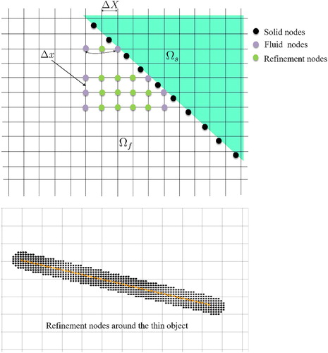
Figure 1. Illustration of the Eulerian and Lagrangian meshes, where $\mathrm{\Omega }s$ and $\mathrm{\Omega }f$ denote the solid region and fluid region, respectively. The velocity interpolation coefficients from the locally refined mesh at the fluid-solid interface are also shown. The velocities at the new nodes are interpolated from the old nodes within the square region.

3.2. Numerical algorithm

In this paper, a monolithic approach is adopted for rigid thin objects FSI system, whereas partitioned approach for elastic objects is applied using the FORTRAN code. The codes are written using FORTRAN language on an Ubuntu 16.04 LTS operating system. VisIt 2.12.3 is an open-source program utilized in this study to visualize most of the 2D simulation results. The VisIt 2.12.3 code can manage large datasets and perform parallel graphical analyses to visualize complex fluid flows.

Table

1. Solve the N-S equations for the entire computational domain using projection method.

2. Compute ${\mathit{d}}_{\mathit{x}}$ and ${\mathit{d}}_{\mathit{y}}$ for the small rectangular region around the thin object with respect to the degree of refinement $dx=DX,DY/2^N$, $d{t}_{new}=DT/2^N$ where $N=1,2,\dots ,n$.

3. Interpolate ${\mathit{u}}_1$ and ${\mathit{v}}_1$ for the boundaries of the rectangular region around the thin object.

4. Compute the boundaries of the refined mesh node around the thin object.

5. Determine the volume fraction for the solid in the local cells and compute the velocity.

6. Compute the momentum exchange.

7. Compute ${\mathit{u}}_{\mathit{d}}$ and ${\mathit{v}}_{\mathit{d}}$ for the volume fraction based on the solid digitizer.

8. Compute the intermediate velocity and pressure

9. Compute ${\mathit{d}}_{\mathit{x}}$ and ${\mathit{d}}_{\mathit{y}}$ and update the values accordingly.

10. Compute the coordinates $\left(x_{pr}\text{and}{y}_{pr}\right)$ for the moving particles using the Crank–Nicholson method.

11. Correct the velocity and pressure.

For elastic structure

12. Compute the (FEM) for solid equations to calculate the space displacement for every time step under the forces from the fluid at Equation (21) after 2-stage correction.

13. Return to Step 1.

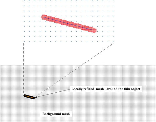
The following validation case was used to check the integration between the AMR and IBM. A preliminary mesh with 30,000 nodes and refined mesh with 6400 nodes were developed using the proposed code. The mesh generator was used to apply the mesh refinement for the two-dimensional simulations. Figure 2 shows the mesh that has been locally refined around a thin object. The main goal here is to observe the dynamic movement of the mesh while eliminating excessive computations within a limited region of the computational domain. There are around 6,400 nodes in the refined mesh within vicinity of the thin object, where $\mathrm{\Delta }t=0.0000625\text{s}$.

Figure 2. Illustration of the background mesh and locally refined mesh within vicinity of the thin object.

4. Simulation set-up

Simulations were conducted to study the characteristics of 2D incompressible viscous flow around a thin object. The size of the computational domain was $20L\times 15L$ while the length of the thin object was L. The leading edge of the thin object was positioned from the inlet at a distance of $(5,7.5)$. Table 1 displays the parameters used to simulate the fluid flow characteristics obtained from IBM. A uniform Cartesian grid was used, where each cell had an equal length and width $(\mathrm{\Delta }x=\mathrm{\Delta }y=0.1)$. The number of nodes was $N_x\times N_y=200\times 150$ while the time step was defined by $\mathrm{\Delta }t=0.005s$. The initial velocity was set as $U_o=1\text{m/s}$. The no-slip conditions at the boundary were defined for the upper and lower boundaries of the targeted domain. The fluid density was set as $\rho =1.0\text{kg/}{\text{m}}^3$ and the $\text{Re}$ was set as 200, following the settings recommended by (Tuanya, Takeuchi, Kajishima, & Ueyama, 2009). The size of the refined mesh zone was $2L\times 1L$, where each cell had an equal length and width of $\mathrm{\Delta }x=\mathrm{\Delta }y=0.00125$. The time step for the refined mesh zone was $0.000625$. The rigid thin object was inclined at three different angles of attack: 15, 30, and 45°. The pressure was set as gradient-free. The thin object was represented by 21 Lagrangian nodal points.

Table 1. Flow around stationary circular cylinder: $C_D$, $C_L$ and St at $R_e=100$.

Source	Drag coefficient, $C_D$	Lift coefficient, $C_L$	Strouhal number, $St$
AMR-IBM	3.255	0.9913	0.2997
(Schäfer & Turek, 1996)	3.22–3.24	0.990–1.010	0.295–0.305
(Verkaik et al., 2014)	3.2258	0.98934	0.30061
(Lee & Lee, 2012)	3.33	1.03	0.299
CFD software	3.227	0.9723	0.2985

5. Results and discussion

AMR enhances resolution to accurately capture flow physics in regions where high flow gradients are expected, such as those within the proximity of the surface of a thin object, which will improve the accuracy of the solution obtained using IBM. The accuracy of the algorithms was firstly verified by comparing the drag coefficient, lift coefficient and Strouhal number of all the algorithms with the results obtained from published reference data, commercial CFD software and the IBM algorithm. The computational time required for the algorithms to complete a task was calculated using the FORTRAN. Laminar flow Re = 100 passing a stationary circular cylinder was used as the benchmark case. Flow passing a thin rigid structure was used to evaluate the capability of the algorithms to simulate FSI with thin objects. The FSI numerical simulation of thin objects in motion was presented to demonstrate the effects of a moving mesh on the developed algorithms. The developed algorithms were implemented and evaluated on flow passing thin elastic structures, which can be easily transformed to address real-world applications, such as the simulation of vocal fold vibrations, two-stroke engine thin valves, insect wings, solar sails and sailing ships. The next section demonstrates the validation of the benchmark case to compute the accuracy and performance of the developed algorithms.

5.1. Validation of benchmark code

The benchmark research of (Schäfer & Turek, 1996) was recalled to validate the developed approach. The Re was set at 100 for laminar flow a round cylinder. For 2D simulations, the Re can be determined based on the cylinder diameter $\left(D\right)$ using the following formula: $\text{Re}=\overline{U}D/v$. The drag coefficient $\left(C_D\right)$ and lift coefficient $\left(C_L\right)$ were calculated based on the simulation results using the following formulas: $C_D=2F_D/\rho U_m^{2}D$ and $C_L=2F_L/\rho U_m^{2}D$. The lift and drag coefficients were determined by integrating the immersed boundary forces with the Lagrangian space. The Strouhal number $\left(St\right)$ was also determined in order to validate the algorithm, which is given by $St=Df/\overline{U}$. The pressure was calculated from the fluid cell closest to the boundary of the cylinder using the pressure interval method. Table 1 shows the lift and drag coefficients as well as the Strouhal numbers obtained for laminar flow around a stationary cylinder at $\mathrm{Re}=100$. 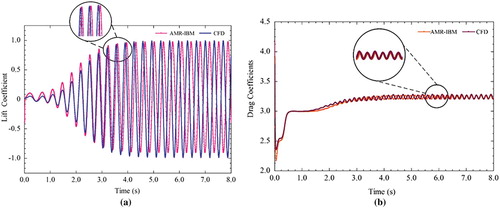It can be relized that the drag coefficients, lift coefficients, and Strouhal numbers obtained from the AMR-IBM algorithm are similar to those obtained by (Lee & Lee, 2012; Schäfer & Turek, 1996; Verkaik, Hulsen, Bogaerds, & van de Vosse, 2014) as well as the CFD software. The visualization of the two graphs shows that the mesh refinements are similar. Figure 3 exhibit an evolution trend for the lift and drag coefficients. The figures demonstrate notable accuracy between the developed AMR–IBM algorithm and the comparable benchmark model for the lift and drag coefficients over the time history of the simulation. From the graphical presentation of the two indicator components, the values are similar to those determined through modeling using the commercial software.

Figure 3. Time-histories of Lift and Drag coefficient AMR-IBM algorithm vs CFD at Re = 100.

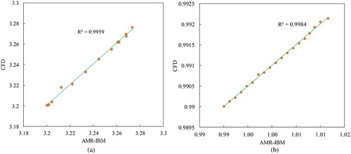
Correlation analysis is performed to ensure validation accuracy. Figure 4 presents the results based on the regression analysis and the correlation coefficient R². The correlation between AMR–IBM and CFD simulation is 99.59% and 99.84% for the drag and lift coefficients, respectively. Hence, the normalized mean root square error (NRMSE) is calculated to support the evidence. The NRMSE calculation value exhibits a slight error of 0.0270, 0.0126, correspondingly. Therefore, this procedure verifies the findings of AMR–IBM by comparing the results with CFD simulation.

Figure 4. The regression analysis for (a) Drag coefficient and (b) lift coefficient factor using AMR-IBM and CFD simulation.

The performance of the developed algorithm was measured by calculating computational time. The calculated computational time for the fine mesh simulation is (209 min), whereas that for the AMR–IBM simulation is (29 min). The primary objective is to reduce computational time, which is achieved by computing the efficiency of the developed algorithm compared with full mesh refinement. The improvement in efficiency is 86.2%. The results exhibit an optimistic outcome in comparison with the benchmark model. The complexity in implementing meshing can be overlooked by the advantage of the extremely short computational time of the developed algorithm.

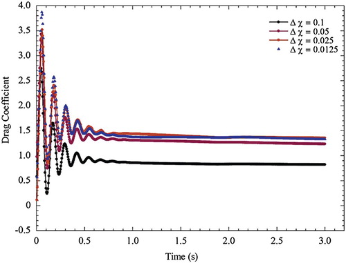
In this research, four different mesh sizes were used to associate the behavior of the proposed algorithm with diverse node sizes. In case number 1, a coarse grid mesh with $\mathrm{\Delta }x$ = 0.1 was used. In the later case, a finer mesh with $\mathrm{\Delta }x$ = 0.05 was used. The third mesh had $\mathrm{\Delta }x$ = 0.025, and the last mesh consisted of $\mathrm{\Delta }x$ = 0.0125. The drag coefficient was comparative in the four cases. Figure 5 shows the drag coefficient curves for different $\mathrm{\Delta }x$. A solution that was close to the converged one for the drag coefficient with the three finer meshes was obtained. The numerical errors presented in thin geometry boundaries caused the shift in C_D values, although drag behavior was the same compared with the others. This finding indicated the requirement for small grid cells to capture thin boundaries. For the grid independence study, Figure 5 shows that the drag coefficients for $\mathrm{\Delta }x$ = 0.0.25 and $\mathrm{\Delta }x$ = 0.0.125 are extremely close. By contrast, the curve of $\mathrm{\Delta }x$ = 0.1 exhibits considerable discrepancies with the others. The minimum cell size should be $\mathrm{\Delta }x$ = 0.025 to reasonably capture the accurate behavior of C_D.

Figure 5. Drag coefficient curves for different $\mathrm{\Delta }x$.

In the AMR–IBM algorithm, mesh layers (each with different cell sizes) are generated in the boundary layer where large flow gradients exist as flow characteristics. Different cases are used to simulate the capability of the developed AMR–IBM algorithm: (1) flow around a stationary rigid infinitely thin object and (2) flow around a stationary thin object inclined at different angles of attack (AMR–IBM). Detailed explanations for the accuracy of AMR–IBM are presented in the following subsection.

5.2. Flow around stationary rigid infinitely thin objects

This section focuses on the performance of the IBM model with a fine mesh in simulating flows around a stationary rigid thin object. The length of the solid (thin object) is smaller than the cell size of the fluid. The simulation outcomes are compared for validation purposes with the AMR–IBM algorithm outcomes.

Figure 6(a) displays the variations of the lift coefficient with time obtained from (Tuanya et al., 2009), the developed AMR–IBM algorithm and the IBM algorithm with a fine mesh. The lift coefficients for the reference data, AMR–IBM algorithm and IBM are 0.749, 0.75 and 0.75, respectively. Figure 6(b) shows the variations of the drag coefficient with time obtained from the developed AMR-IBM algorithm and the IBM model with a fine mesh. The drag coefficients for the AMR–IBM algorithm and IBM CFD are 1.31 and 1.35, respectively. The drag coefficient error between AMR–IBM and IBM is 2.96%, which indicates an acceptable accuracy between the computed drag coefficient for the developed algorithm and the IBM model.

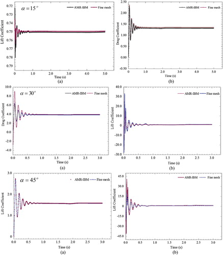
Figure 6. Variations of the (a) lift coefficient and (b) drag coefficient with time for flow around a stationary rigid thin object at $R_e=200$ obtained using the AMR-IBM algorithm. The lift and drag coefficients obtained from the IBM algorithm with full mesh refinement are plotted for comparison.

In general, the results obtained from the developed AMR–IBM algorithm and the IBM algorithm with a fine mesh exhibit good agreement. However, the developed AMR–IBM algorithm is more favorable because of its efficiency, which eliminates high-level computations and is less time-consuming. The AMR–IBM algorithm is suitable for solving real-world FSI problems, such as flow passing an aerofoil and the flapping of insect wings.

5.3. Flow around stationary infinitely thin objects inclined at different angles of attack

In this case, the developed AMR–IBM algorithm was used to simulate the flow around a stationary thin object inclined at different angles of attack, such as 30° and 45°. Flow was fully developed at t = 3 s. Different angles of attack were used to emulate flapping insect wings and other applications. Figure 6 shows the variations of the lift and drag coefficients with time obtained from the developed AMR–IBM algorithm and the IBM algorithm with a fine mesh at different angles of attack, namely, 30° and 45°. The lift coefficients for the AMR–IBM algorithm and the IBM algorithm with a fine mesh are 0.95, 0.97, 1.10 and 1.15. The drag coefficients for the AMR–IBM algorithm and the IBM with a fine mesh are 3.94, 3.84, 1.588 and 1.576.

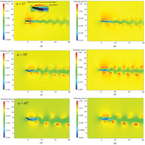
Figure 7 shows the velocity contour of flow around the stationary rigid thin object at t = 8 s. Average pressure on the surface considerably increased because the flow in the computational domain was subjected to a sudden increase due to the inclination of the thin object with respect to the free-stream direction, thereby leading to fluctuations in the force acting on the object. The velocity field in the computational domain and the velocity field close to the thin object inclined at = 15°, 30° and 45° are clearly shown in Figure 7. The location of the finest mesh is evident in Figure 7(a). In addition, Figure 7(a) were used to compare the velocity field to the fine mesh velocity field result in Figure 7(b). The comparison shows an acceptable visual agreement between the two velocity fields.

Figure 7. Velocity contour for flow around a stationary rigid thin object (a) AMR-IBM algorithm, (b) Fine mesh.

However, for FSI problems involving moving objects (where are large deformations on the surface of the thin objects), the mesh needs to update regularly to capture changes in the implicit boundary line. In such scenarios, it is advantageous to generate a thin mesh layer within proximity of the boundaries of the thin object such that an optimal mesh is preserved in the boundary layer at all times. The performance of the AMR-IBM algorithm in dealing with 2D incompressible viscous laminar flows around a moving thin object is presented in the following section.

5.4. Flow around moving infinitely thin objects inclined at different angles of attack

The capability of the AMR-IBM algorithm in simulating flow around a moving thin object was assessed and the results are presented and discussed in this section. The size of the computational domain is the same as that in the earlier case. Likewise, the point of origin for the thin object in the computational domain is the same as that in the earlier situation. The rigid thin object (represented by 21 Lagrangian nodal points) was inclined at three different angles of attack: 15°, 30°, and 45°. The pressure at the outlet of the computational domain was set as gradient-free. The Reynolds number was fixed for all the simulations. The two edges of the thin object were unconstrained, enabling the object to move. The refined mesh around the boundaries of the thin object changes dynamically in response to the motion of the object. Figure 8 show the velocity contours obtained for incompressible viscous laminar flow around a moving thin object at different time steps $t=1.5s,3.5s,8.0s$ for three angles of attack. The following motions were observed from the simulations: (1) rotation of the thin object around its center of gravity and (2) motion of the thin object in the fluid domain. In general, the thin object rotates and revolves in the clockwise direction with respect to time. The fluid forces push the thin object in the horizontal direction whereas the forces resulting from the pressure difference between the upper and lower surfaces lift the thin object as the simulation progresses. It is worth noting that even though the thin object represents an aerofoil in the simulations, the thin object is not only limited to aerofoil, but it can also represent other objects such as small fish fins, various types of insect wings, and aortic valves. In this study, the focus is on the response of the thin object due to the fluid forces acting on it. The flow dynamics were solved using a fixed Cartesian mesh, where the flow properties were interpolated between the adjacent cells using IBM. The overall fluid force acting on the immersed boundary was calculated by extrapolation from the mesh points and used as the external force to the structural dynamic’s solver.

Figure 8. Velocity contour of the moving thin object inclined at an angle of attack 45° at (a) t = 1.5 s, (b) t = 3.5 s, and (c) t = 8.0 s obtained using the AMR-IBM algorithm.

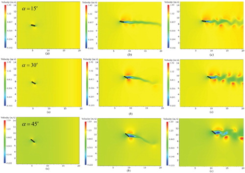
Figure 8 shows the final position of the thin object at different angles of attack (15°, 30° and 45°) at t = 8 s. The position of the thin object was considerably different due to the varying angles of attack. The angle of attack affected the drag and lift forces acting on the thin object, which in turn, affected its position. The rotation of the thin object around its center of gravity reduced this effect over time.

The performance of the developed algorithm was measured by calculating computational time. The calculated computational times for the fine mesh simulation at different angles of attack, namely, 15°, 30° and 45° are 2760, 2776 and 2794 min, respectively, whereas the computational times for the AMR–IBM simulation are 45, 49 and 50 min, respectively. This study aims to reduce computational time, which is achieved by computing the efficiency of the developed algorithm compared with a fine mesh. The improvement in efficiency was estimated as 98.2%. The results showed an optimistic outcome compared with the IBM algorithm with a full refinement mesh for moving thin objects at different angles of attack (15°, 30° and 45°). The complexity in implementing meshing can be overlooked by the advantage of the extremely short computational time of the developed algorithm.

In the second application, the developed AMR algorithm for the immersed solid approach was coupled with FEM for structure interaction case involving a deformable elastic object in a fluid. The problem because of the integrating an elastic effect the dynamics of the fluid, and various approaches, such as the full Eulerian approach, are available.

A simplified model, which consists of a 2D thin elastic solid (beam) immersed in a viscous incompressible fluid, was established to demonstrate the applicability of the AMR–IBFEM algorithm. This algorithm was written in FORTRAN language on an Ubuntu 16.04 LTS operating system and could easily capture pressure discontinuities across interfaces, which coincided with the thin elastic structure in reducing computational time. The investigated problem retains important physical features, such as large deformations, which are common in many complex models. In the next section, the AMR–IBFEM algorithm is implemented on elastic applications, the problem related to a flexible filament is addressed. A flexible filament was used to model the flag-flapping phenomenon, to understand the locomotion of aquatic animals and microorganisms and to investigate the movement of a filament in a soap bubble film.

5.5. AMR-IBFEM model of a flexible filament application

Flexible filament models are complex due to their high elasticity and thin boundary layers. The fluid resistance and the gravity acceleration were not considered in the present work. A filament may settle in a overextended straight state depending on the parameters used. The geometrical domain and boundary conditions are described in Figure 9. The AMR–IBFEM mesh used to analyses a filament was modeled exactly as a beam with 201 geometric elements. One end of the beam, denoted as (A) in Figure 9, is fixed. Perturbation was introduced into the system by tilting the filament at an angle towards the horizontal direction at time t = 0. Each cell had an equal length and width $\mathrm{\Delta }x=\mathrm{\Delta }y=0.1$. The settings used for the simulations of a 2D laminar flow passing a flexible filament are described in this section. The number of nodes was $N_x\times N_y=200\times 150$, and the time step was defined by $\mathrm{\Delta }t=0.005s$. The initial velocity was set as $U_o=1\text{m/s}$. ‘No slip’ boundary conditions were defined for the upper and lower walls of the computational domain. Fluid density was set as $\rho =1.0\text{kg/}{\text{m}}^3$, and Re was set as 200. The size of the refined mesh zone was $1.5\text{m}\times 0.25\text{m}$, where each cell had an equal length and width of $\mathrm{\Delta }x=\mathrm{\Delta }y=0.00625$. The number of nodes was $n_x\times n_y=240\times 80$. The time step for the refined mesh zone was $0.0003125s$. The flexible filament was positioned at the center of the domain at an axial distance of 4.5 m from the inlet. The length of the thin elastic structure was 1 m, and the structure was composed of 201 elements. The Poisson’s ratio and Young’s modulus of the thin elastic structure were set as 0.30 and 3.0 MPa, respectively.

Figure 9. The domain and boundary conditions for the flexible filament 2D problem.

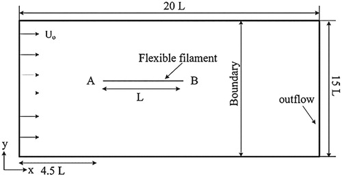
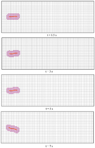
Figure 10 shows the result of the deformed flexible filament at different time steps with mesh refinement around the thin object. In the beginning of the simulation, the object stretched straight wide open in the direction of flow. Then, the filament started to follow the characteristics of fluid flow due to the high elasticity of the thin object.

Figure 10. Snapshots of the deformed flexible filament at different time steps. Note that a fixed mesh was used for the fluid flow whereas an adaptive mesh is used within proximity of the thin elastic structure to capture the physics of fluid-solid interaction.

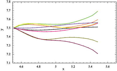
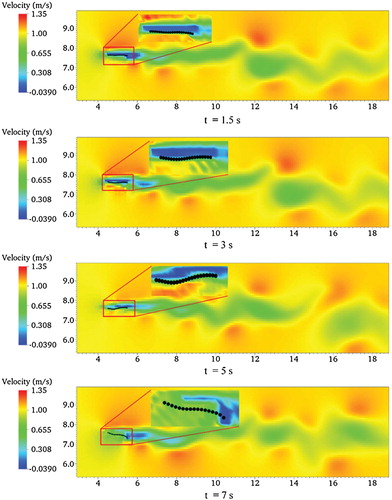
The filament was fixed at its edge. For a low Re, the filament exhibited passive pitching in terms of its natural bending modes. The deflection envelope and time history of the tip displacement are plotted in Figure 11. At Re = 200, the shear layers passing the filament and refinement meshed and formed the fluid flow, which evolved with time and increased in strength. Subsequently, flow was converted over the flexible filament, triggered vibrations and shed downstream of the thin structure in the form of a vortex street with alternate shedding vortices. The filament started vibrating in its first mode shape when the force of flow started to convert. However, the filament attained a mixed-mode vibration between its first and second mode shapes once the fluid flow impinged on it and started shedding from the trailing edge. Figure 11 shows the flapping motion of a single filament immersed in fluid at different times. The filament was clearly restricted to the fluid flow features. Lagrangian coherent structures were presented in the near field along with the velocity contours to obtain considerable insights into flow interactions. Close-up views of the velocity fields near the interface are depicted in Figure 11 to observe filament movement.

Figure 11. Flapping motion of a single filament immersed in fluid.

The impingement of fluid flow on the elastic filament caused it to change manners because of the impingement position and the Strouhal frequency of the fluctuating fluid flow vectors. Vortex–filament interactions and the evolution of the trailing edge flow topology were investigated on the basis of velocity contours at different time steps, as shown in Figure 12. Mesh refinement was obtained by plotting the backward finite time of the velocity field, which clearly showed how the impingement of fluid flow caused the filament to bend in different modes, thereby augmenting propulsive efficiency.

Figure 12. Two-dimensional flexible filament on velocity and geometry deformation distribution at different time step.

6. Conclusions

A combined AMR and cut cell-IBM with the two-stage pressure-velocity correction is developed to simulate flows at the fluid-structure interface for thin objects. In the elastic structures, cut-cell IBM with pressure-velocity correction is integrated with FEM and AMR is developed to attain high resolution of the flow characteristics within the area near the surface of the thin elastic object. Local adaptive mesh refinement is computed to achieve high resolution of the flow physics within the vicinity of the surface of thin objects where large flow gradients are expected while retaining a moderate resolution at other regions of the computational domain. The algorithms are developed to simulate 2D laminar flows around stationary and moving arbitrary shaped rigid and elastic thin structures. The flow passing a cylinder is designated as the benchmark case to validate the numerical model, and a few numerical cases are provided to determine the performance and accuracy of the algorithm. The results prove the accuracy of the established algorithms in simulating flow characteristics in the boundary layers of thin structures. These algorithms can simulate uniform flows around various thin, rigid structures, including sharp-edged objects. In general, the algorithm performs satisfactorily, providing fast, reliable results, in which computational time is shortened to 98.3% in the case of a thin rigid object compared with non-adaptive fine grid. The proposed algorithms can be successfully applied to solve complex FSI problems.

Disclosure statement

No potential conflict of interest was reported by the authors.

ORCID

Zaher Mundher Yaseen http://orcid.org/0000-0003-3647-7137

References

- Akbarian, E., Najafi, B., Jafari, M., Faizollahzadeh Ardabili, S., Shamshirband, S., & Chau, K. (2018). Experimental and computational fluid dynamics-based numerical simulation of using natural gas in a dual-fueled diesel engine. Engineering Applications of Computational Fluid Mechanics, 12(1), 517–534. doi: 10.1080/19942060.2018.1472670
- Aldlemy, M. S., Rasani, M., Ya, T. M. Y. S., & Ariffin, A. K. (2018). Dynamic adaptive mesh refinement of fluid structure interaction using immersed boundary method with two stage corrections. Scientia Iranica. doi: 10.24200/sci.2018.50347.1650
- Angot, P., Bruneau, C.-H., & Fabrie, P. (1999). A penalization method to take into account obstacles in incompressible viscous flows. Numerische Mathematik, 81(4), 497–520. doi: 10.1007/s002110050401
- Bailoor, S., Annangi, A., Seo, J. H., & Bhardwaj, R. (2017). Fluid–structure interaction solver for compressible flows with applications to blast loading on thin elastic structures. Applied Mathematical Modelling, 52, 470–492. doi: 10.1016/j.apm.2017.05.038
- Bao, Y., Donev, A., Griffith, B. E., McQueen, D. M., & Peskin, C. S. (2017). An immersed boundary method with divergence-free velocity interpolation and force spreading. Journal of Computational Physics, 347, 183–206. doi: 10.1016/j.jcp.2017.06.041
- Boukharfane, R., Eugênio Ribeiro, F. H. E., Bouali, Z., & Mura, A. (2018). A combined ghost-point-forcing/direct-forcing immersed boundary method (IBM) for compressible flow simulations. Computers & Fluids, 162, 91–112. doi: 10.1016/j.compfluid.2017.11.018
- Bourlet, T. F., Gurugubelli, P. S., & Jaiman, R. K. (2015). The boundary layer development and traveling wave mechanisms during flapping of a flexible foil. Journal of Fluids and Structures, 54, 784–801. doi: 10.1016/j.jfluidstructs.2015.01.013
- Breugem, W.-P., van Dijk, V., & Delfos, R. (2012). An efficient immersed boundary method based on penalized direct forcing for simulating flows through real porous media. ASME 2012 fluids engineering division summer meeting collocated with the ASME 2012 heat transfer summer conference and the ASME 2012 10th international conference on nanochannels, microchannels, and minichannels (pp. 1407–1416).
- de Tullio, M. D., & Pascazio, G. (2016). A moving-least-squares immersed boundary method for simulating the fluid–structure interaction of elastic bodies with arbitrary thickness. Journal of Computational Physics, 325, 201–225. doi: 10.1016/j.jcp.2016.08.020
- Favier, J., Revell, A., & Pinelli, A. (2016). Fluid structure interaction of multiple flapping filaments using Lattice Boltzmann and immersed boundary methods. In Advances in fluid-structure interaction (pp. 167–178). Cham: Springer.
- Frantzis, C., & Grigoriadis, D. G. E. (2019). An efficient method for two-fluid incompressible flows appropriate for the immersed boundary method. Journal of Computational Physics, 376, 28–53. doi: 10.1016/j.jcp.2018.09.035
- Fujisawa, K., & Asada, A. (2016). Nonlinear parametric sound enhancement through different fluid layer and its application to noninvasive measurement. Measurement: Journal of the International Measurement Confederation, 94, 726–733. doi: 10.1016/j.measurement.2016.09.004
- Ghalandari, M., Koohshahi, E. M., Shamshirband, S., & Chau, K. W. (2019). Mechanics numerical simulation of nanofluid flow inside a root canal, 2060. doi: 10.1080/19942060.2019.1578696
- Gilmanov, A., Le, T. B., & Sotiropoulos, F. (2015). A numerical approach for simulating fluid structure interaction of flexible thin shells undergoing arbitrarily large deformations in complex domains. Journal of Computational Physics, 300, 814–843. doi: 10.1016/j.jcp.2015.08.008
- Goza, A., & Colonius, T. (2017). A strongly-coupled immersed-boundary formulation for thin elastic structures. Journal of Computational Physics, 336, 401–411. doi: 10.1016/j.jcp.2017.02.027
- Griffith, M. D., & Leontini, J. S. (2017). Sharp interface immersed boundary methods and their application to vortex-induced vibration of a cylinder. Journal of Fluids and Structures, 72, 38–58. doi: 10.1016/j.jfluidstructs.2017.04.008
- Griffith, B. E., & Luo, X. (2017). Hybrid finite difference/finite element immersed boundary method. International Journal for Numerical Methods in Biomedical Engineering, 33(12), 1–46. doi: 10.1002/cnm.2888
- Horng, T.-L., Hsieh, P.-W., Yang, S.-Y., & You, C.-S. (2018). A simple direct-forcing immersed boundary projection method with prediction-correction for fluid-solid interaction problems. Computers & Fluids, 176, 135–152. doi: 10.1016/j.compfluid.2018.02.003
- Kajishima, T., & Taira, K. (2017). Finite-difference discretization of the advection-diffusion equation. In Computational fluid dynamics (pp. 23–72). Cham: Springer.
- Kajishima, T., & Takeuchi, S. (2013). Simulation of fluid-structure interaction based on an immersed-solid method. Journal of Mechanical Engineering and Sciences, 5 (unknown), 555–561. doi: 10.15282/jmes.5.2013.1.0052
- Kajishima, T., Takiguchi, S., Hamasaki, H., & Miyake, Y. (2001). Turbulence structure of particle-laden flow in a vertical plane channel due to vortex shedding. JSME International Journal Series B, 44(4), 526–535. doi: 10.1299/jsmeb.44.526
- Kempe, T., & Frohlich, J. (2012). An improved immersed boundary method with direct forcing for the simulation of particle laden flows. Journal of Computational Physics, 231(9), 3663–3684. doi: 10.1016/j.jcp.2012.01.021
- Kevlahan, N. K.-R., & Ghidaglia, J.-M. (2001). Computation of turbulent flow past an array of cylinders using a spectral method with Brinkman penalization. European Journal of Mechanics-B/Fluids, 20(3), 333–350. doi: 10.1016/S0997-7546(00)01121-3
- Kirkpatrick, M. P., Armfield, S. W., & Kent, J. H. (2003). A representation of curved boundaries for the solution of the Navier–Stokes equations on a staggered three-dimensional Cartesian grid. Journal of Computational Physics, 184(1), 1–36. doi: 10.1016/S0021-9991(02)00013-X
- Lee, J., & Lee, S. (2012). Fluid–structure interaction analysis on a flexible plate normal to a free stream at low Reynolds numbers. Journal of Fluids and Structures, 29, 18–34. doi: 10.1016/j.jfluidstructs.2011.12.012
- Lee, L., & LeVeque, R. J. (2003). An immersed interface method for incompressible Navier–Stokes equations. SIAM Journal on Scientific Computing, 25(3), 832–856. doi: 10.1137/S1064827502414060
- Liang, Z., Wei, L., Lu, J., & Qin, X. (2017). Numerical simulation of a two-dimensional flapping wing in advanced mode. Journal of Hydrodynamics, 29(6), 1076–1080. doi: 10.1016/S1001-6058(16)60801-6
- Lin, X., He, G., He, X., & Wang, Q. (2018). Dynamic response of a semi-free flexible filament in the wake of a flapping foil. Journal of Fluids and Structures, 83, 40–53. doi: 10.1016/j.jfluidstructs.2018.08.009
- Liu, J., Zhao, N., Hu, O., Goman, M., & Li, X. K. (2013). A new immersed boundary method for compressible Navier–Stokes equations. International Journal of Computational Fluid Dynamics, 27(3), 151–163. doi: 10.1080/10618562.2013.791391
- Martínez-Ferrer, P. J., Qian, L., Ma, Z., Causon, D. M., & Mingham, C. G. (2018). An efficient finite-volume method to study the interaction of two-phase fluid flows with elastic structures. Journal of Fluids and Structures, 83, 54–71. doi: 10.1016/j.jfluidstructs.2018.08.019
- Maxian, O., Kassen, A. T., & Strychalski, W. (2018). A continuous energy-based immersed boundary method for elastic shells. Journal of Computational Physics, 371, 333–362. doi: 10.1016/j.jcp.2018.05.045
- Miao, S., Hendrickson, K., & Liu, Y. (2017). Computation of three-dimensional multiphase flow dynamics by fully-coupled immersed flow (FCIF) solver. Journal of Computational Physics, 350, 97–116. doi: 10.1016/j.jcp.2017.08.042
- Mittal, R., & Iaccarino, G. (2005). Immersed boundary methods. Annual Review of Fluid Mechanics, 37(1), 239–261. doi: 10.1146/annurev.fluid.37.061903.175743
- Mo, H., Lien, F.-S., Zhang, F., & Cronin, D. S. (2018). An immersed boundary method for solving compressible flow with arbitrarily irregular and moving geometry. International Journal for Numerical Methods in Fluids, 88(5), 239–263. doi: 10.1002/fld.4665
- Mori, Y., & Peskin, C. S. (2008). Implicit second-order immersed boundary methods with boundary mass. Computer Methods in Applied Mechanics and Engineering, 197(25–28), 2049–2067. doi: 10.1016/j.cma.2007.05.028
- Mou, B., He, B.-J., Zhao, D.-X., & Chau, K. (2017). Numerical simulation of the effects of building dimensional variation on wind pressure distribution. Engineering Applications of Computational Fluid Mechanics, 11(1), 293–309. doi: 10.1080/19942060.2017.1281845
- Muralidharan, B., & Menon, S. (2018). Simulation of moving boundaries interacting with compressible reacting flows using a second-order adaptive Cartesian cut-cell method. Journal of Computational Physics, 357, 230–262. doi: 10.1016/j.jcp.2017.12.030
- Nasar, A. M. A., Rogers, B. D., Revell, A., Stansby, P. K., & Lind, S. J. (2019). Eulerian weakly compressible smoothed particle hydrodynamics (SPH) with the immersed boundary method for thin slender bodies. Journal of Fluids and Structures, 84, 263–282. doi: 10.1016/j.jfluidstructs.2018.11.005
- Peskin, C. S. (1972). Flow patterns around heart valves: A numerical method. Journal of Computational Physics, 10(2), 252–271. doi: 10.1016/0021-9991(72)90065-4
- Peskin, C. S. (1977). Numerical analysis of blood flow in the heart. Journal of Computational Physics, 25(3), 220–252. doi: 10.1016/0021-9991(77)90100-0
- Peskin, C. S., & McQueen, D. M. (1989). A three-dimensional computational method for blood flow in the heart I. Immersed elastic fibers in a viscous incompressible fluid. Journal of Computational Physics, 81(2), 372–405. doi: 10.1016/0021-9991(89)90213-1
- Ramezanizadeh, M., Alhuyi Nazari, M., Ahmadi, M. H., & Chau, K. (2019). Experimental and numerical analysis of a nanofluidic thermosyphon heat exchanger. Engineering Applications of Computational Fluid Mechanics, 13(1), 40–47. doi: 10.1080/19942060.2018.1518272
- Rasani, M. R., Aldlemy, M. S., & Harun, Z. (2017). Fluid-structure interaction analysis of rear spoiler vibration for energy harvesting potential. Journal of Mechanical Engineering and Sciences, 11(1), 2415–2427. doi: 10.15282/jmes.11.1.2017.2.0223
- Riahi, H., Meldi, M., Favier, J., Serre, E., & Goncalves, E. (2018). A pressure-corrected immersed boundary method for the numerical simulation of compressible flows. Journal of Computational Physics, 374, 361–383. doi: 10.1016/j.jcp.2018.07.033
- Schäfer, M., & Turek, S. (1996). Benchmark computations of laminar flow around a cylinder. In Flow Simulation with High-Performance Computers II, Volume 52 of Notes on Numerical Fluid Mechanics, Vieweg, 52 (pp. 547–566). doi: 10.1007/978-3-322-89849-4_39
- Schott, B., Ager, C., & Wall, W. A. (2018). Monolithic cut finite element based approaches for fluid-structure interaction. ArXiv Preprint ArXiv:1807.11379.
- Sotiropoulos, F., & Yang, X. (2014). Immersed boundary methods for simulating fluid – structure interaction. Progress in Aerospace Sciences, 65, 1–21. doi: 10.1016/j.paerosci.2013.09.003
- Su, S.-W., Lai, M.-C., & Lin, C.-A. (2007). An immersed boundary technique for simulating complex flows with rigid boundary. Computers & Fluids, 36(2), 313–324. doi: 10.1016/j.compfluid.2005.09.004
- Tian, F.-B., Dai, H., Luo, H., Doyle, J. F., & Rousseau, B. (2014). Fluid–structure interaction involving large deformations: 3D simulations and applications to biological systems. Journal of Computational Physics, 258, 451–469. doi: 10.1016/j.jcp.2013.10.047
- Tuanya, T. M. Y. S., Takeuchi, S., Kajishima, T., & Ueyama, A. (2009). Technical note: Immersed boundary method (body force) for flow around thin bodies with sharp edges. International Journal of Mechanical and Materials Engineering, 4(1), 98–102.
- Udaykumar, H. S., Mittal, R., Rampunggoon, P., & Khanna, A. (2001). A sharp interface Cartesian grid method for simulating flows with complex moving boundaries. Journal of Computational Physics, 174(1), 345–380. doi: 10.1006/jcph.2001.6916
- Uhlmann, M. (2005). An immersed boundary method with direct forcing for the simulation of particulate flows. Journal of Computational Physics, 209(2), 448–476. doi: 10.1016/j.jcp.2005.03.017
- Vadala-Roth, B., Rossi, S., & Griffith, B. E. (2018). Stabilization approaches for the hyperelastic immersed boundary method for problems of large-deformation incompressible elasticity. ArXiv Preprint ArXiv:1811.06620.
- Verkaik, A. C., Hulsen, M. A., Bogaerds, A. C. B., & van de Vosse, F. N. (2014). An overlapping domain technique coupling spectral and finite elements for fluid flow. Computers & Fluids, 100, 336–346. doi: 10.1016/j.compfluid.2014.05.026
- Wall, W. A., Gerstenberger, A., & Mayer, U. M. (2009). Advances in fixed-grid fluid structure interaction. ECCOMAS Multidisciplinary Jubilee Symposium, 14, 235–249. Retrieved from http://www.springerlink.com/index/J72P233005314362.pdf doi: 10.1007/978-1-4020-9231-2_16
- Wang, L., Currao, G. M. D., Han, F., Neely, A. J., Young, J., & Tian, F.-B. (2017). An immersed boundary method for fluid–structure interaction with compressible multiphase flows. Journal of Computational Physics, 346, 131–151. doi: 10.1016/j.jcp.2017.06.008
- Wang, W.-Q., Yan, Y., & Tian, F.-B. (2017). A simple and efficient implicit direct forcing immersed boundary model for simulations of complex flow. Applied Mathematical Modelling, 43, 287–305. doi: 10.1016/j.apm.2016.10.057
- Ya, T. M. Y. S. T., Takeuchi, S., & Kajishima, T. (2007). Immersed boundary and finite element methods approach for interaction of an elastic body and fluid by Two-stage correction of velocity and pressure. ASME/JSME 2007 5th joint fluids engineering conference (pp. 75–81).
- Yang, J., Yu, F., Krane, M., & Zhang, L. T. (2018). The Perfectly Matched layer absorbing boundary for fluid – structure interactions using the immersed finite element method. Journal of Fluids and Structures, 76, 135–152. doi: 10.1016/j.jfluidstructs.2017.09.002
- Ye, T., Mittal, R., Udaykumar, H. S., & Shyy, W. (1999). An accurate Cartesian grid method for viscous incompressible flows with complex immersed boundaries. Journal of Computational Physics, 156(2), 209–240. doi: 10.1006/jcph.1999.6356
- Yoshihiko, Y., Shintaro, T., & Takeo, K. (2007). Efficient immersed boundary method for Strong interaction problem of arbitrary shape object with the Self-Induced flow. Journal of Fluid Science and Technology, 2(1), 1–11. doi: 10.1299/jfst.2.1
- Zhu, L., & Peskin, C. S. (2002). Simulation of a flapping flexible filament in a flowing soap film by the immersed boundary method. Journal of Computational Physics, 179, 452–468. doi: 10.1006/jcph.2002.7066