Numerical simulation of flow over ogee crested spillways under high hydraulic head ratio

ABSTRACT

Ogee spillway is one of the most common types of the spillway. Researchers have attempted to investigate the hydraulics of ogee structure under hydraulic heads near the design head. Herein, an ogee-crested spillway is studied at heads significantly greater than the design head. The efforts are undertaken to study the hydrodynamic field under high head ratio conditions by conducting a numerical simulation using OpenFOAM with five turbulence closures including standard k–ε, realizable k–ε, RNG k–ε, k–ω SST and LRR. The comparisons of flow parameters under different head ratios with the experimental data demonstrated that the LRR model had the best performance, which shows its strength in cases dealing with flow separation or significant streamline curvature. It is found that with increasing hydraulic head, up to seven times that of the design head, the flow separation zone grows linearly. Discharge coefficients are studied for a wide range of head ratios. It is concluded that increasing head ratio up to five leads to an increase in the discharge coefficient due to decreasing pressure on the ogee crest. As head ratio increases to greater values, the discharge coefficient drops suddenly due to some changes in the pressure field.

KEYWORDS:

• Numerical modeling
• ogee spillway
• high head ratio
• turbulence models
• OpenFOAM

Introduction

Spillways are designed for dams to release excess water or floods that cannot be contained in the storage volume. Using a spillway, the excess water flows from the top of the reservoir and is carried through a constructed waterway back to the river (The U.S. Bureau of Reclamation [USBR], 1987). Many dam-break events have been caused due to improperly designed spillways or insufficient spillway capacity.

By definition, the crest profile of ogee spillways corresponds to the trajectory of the lower nappe of a free ventilated sharp-crested weir (Hager, 1987). These weirs are thus designed for a single precise value of the upstream head, which is called the design head. Ogee crested spillways are routinely designed to operate with upstream heads up to (or slightly higher than) the design head. The discharge over an ogee crest is strongly influenced by the ratio of the actual head to the design head. When the reservoir level is below the design head, positive relative pressures develop over the spillway. In this case, the water flows over the crest without any significant resistance to the crest surface, meaning that the discharge coefficient increases for heads lower than the design head. For heads greater than the design head, sub-atmospheric or negative pressure develops along the crest at the interface between the flow and the spillway crest, resulting in suction, which causes the discharge coefficient to increase. Vermeyen (1992) showed that under an ideal entrance condition, the discharge coefficient continues to increase for heads five times the design head. It should be noted that this happens mostly under specific conditions where abutment effects are not present (reservoir and crest with the same width), and when sidewalls prevent air supply to the bottom part of the nappe.

In addition, when the pressure falls locally below the water vapor pressure, it leads to risk of cavitation damage, and may cause flow detachment in case of connection of the lower part of the nappe with the atmosphere (Erpicum et al., 2018). Such risks cannot be accepted on a real spillway. On a physical scale model, as the atmospheric pressure is usually not scaled, cavitation does not appear, or appears later than it would on a real-sized structure.

USBR (1987) studied the behavior of water flow over spillways through comprehensive laboratory experiments that led to developing and publishing spillway design manuals. Moreover, USBR (2014) has standardized and documented the technical process of designing spillways and technical references for the evaluation of spillways through different design standards.

Apart from these fundamental studies, many researchers have attempted to implement experimental and numerical models to predict the hydraulics of ogee crest structure. Physical studies are typically costly and prone to scale effects. Chatila and Tabbara (2004), Johnsen and Savage (2006) and Kanyabujinja (2015) have performed limited experiments, mostly for their numerical model verification. Peltier, Dewals, Archambeau, Pirotton, and Erpicum (2018) performed velocity and pressure measurements in experimental modeling of ogee spillways for heads significantly more than the design head.

On the other hand, numerical modeling can be a valid and affordable method to study this problem in the presence of complex geometry (Chau & Jiang, 2004; Quezada, Tamburrino, & Nino, 2018; Wu and Chau, 2006). Savage and Johnson (2001) applied the finite element CFD package Flow-3D using variable-sized hexahedral cells to calculate flow parameters over an ogee crested spillway. They found a reasonable agreement between their numerical model and experimental data available in the literature for both pressure and discharge. Then, Johnsen and Savage (2006) extended their investigation to study the influence of tailwater on the ogee spillway. Chatila and Tabbara (2004) predicted the water free surface over the ogee spillway by applying a finite element CFD software called ADINA. They used the k–ε turbulence model and a triangular mesh and verified their 2DV numerical results with their benchmark data measured in the laboratory. Kim and Park (2005) applied the Flow-3D model using RNG k–ε turbulence model to investigate the pressure and velocity distribution over the ogee spillways considering surface roughness effects. Bhajantri, Eldho, and Deolalikar (2006) considering weakly compressible flow, developed their 2D CFD code using finite volume method to model flow on the ogee spillway. A study of flow over an ogee-crested fish bypass was done by Turan, Carrica, Lyons, Hay, and Weber (2008). They applied the CFD code Fluent with a standard k–ε turbulence closure and structured/unstructured hybrid grid to simulate free surface and velocities in complex 3D hydraulic structures including gates and aeration slots. A numerical simulation was undertaken by Chanel and Doering (2008) on three case studies with different ratios of spillway height to the design head using the CFD software Flow-3D. Kanyabujinja (2015) used a two-phase CFD package Ansys-Fluent with realizable k–ε eddy viscosity closure and modeled flow domain of a typical ogee spillway, in two and three dimensions. A 2DV meshless Lagrangian model based on weakly compressible Moving particle Semi-implicit (MPS) method was developed by Jafari-Nodoushan, Hosseini, Shakibaeinia, and Mousavi (2016) to simulate pressure and velocity over ogee crest spillways. In a recent study, Fleit, Baranya, and Bihs (2018) introduced a numerical model, REEF3D, to predict water level and flow domain on an ogee type weir for both conditions of free surface and submerged flow.

The literature review shows that there are some gaps in the knowledge of ogee crest spillways. First, in the context of numerical studies of flow over ogee crested spillways under high hydraulic head ratio, and second, the absence of a detailed assessment of the performance of different turbulence models for simulating flow characteristics of ogee spillways. Although several researchers have applied advanced software or developed codes equipped with various turbulence models, they have focused on specific hydraulic conditions in which the hydraulic head is lower than the design head or in some cases, slightly greater than the design head. As mentioned previously, the ratio of actual head to design head is an important factor that affects the discharge coefficient of ogee crests considerably. Therefore, the condition in which the head is significantly larger than the design head needs to be further studied.

In the present paper, the OpenFOAM numerical package is applied to investigate the ogee-crested spillways operating at hydraulic heads significantly higher than the design head using Navier–Stokes equations. The main goal of this study is to determine to what extent chosen turbulence closures can improve hydraulic domain prediction along the ogee spillway crest. According to the above literature review, five widely used efficient turbulence models were chosen in order to evaluate the performance of efficient Reynolds Averaged Navier Stokes (RANS) models in simulation of flow over ogee crested spillways under high hydraulic head ratio and their potential capacity for practical design applications. These five RANS models (standard k–ε, realizable k–ε, RNG k–ε, k–ω SST and LRR) have been chosen due to their extensive usage and competitive advantages compared with other turbulence closures like Large Eddy Simulations (LES) models. For engineering cases, application of LES approaches is still not practical due to the heavy computational cost. Thus, the practice of RANS simulations is still meaningful in the field of hydraulic studies of flow over ogee spillways.

Therefore, the present study first evaluates the performance of five various turbulence models (standard k–ε, RNG k–ε, realizable k–ε, k–ω SST and LRR) models versus experimental data on the flow field over an ogee crested spillway at heads significantly higher than the design head using 2DV OpenFOAM; and then carries out additional computations to assess how varying hydraulic head ratio affects the flow discharge and water free surface.

Within the framework depicted above, the rest of the paper is organized as follows: In the second section, the structure of the numerical model including governing equations and turbulent closures are presented. The case studies and model verification are described in the third section. The numerical model results and discussions are explained in the fourth section. Finally, the study closes with some concluding remarks in the last section.

Methodology

Flows over spillways have been investigated widely by numerical simulation, which has been one of the most useful tools to study fluid-structure interaction in the past years. To model flow over the ogee spillway under high hydraulic head ratio in the present study, the OpenFOAM framework was employed. OpenFOAM (Open Field Operation And Manipulation) is a free, open source computational fluid dynamics (CFD) software package developed using C++. Most hydraulic engineering problems can be modeled by it (Shaheed, Mohammadian, & Kheirkhah Gildeh, 2018). OpenFOAM has the capability of simulating the flow field by executing several turbulence models and various numerical schemes.

Governing equations

The equations for continuity and momentum conservation for incompressible flows can be written as follows (Chau & Jiang, 2001; Holzmann, 2017): (1) $\begin{array}{rl}\mathrm{\nabla }.\mathit{U}& =0\end{array}$(1) (2) $\begin{array}{rl}\frac{\mathrm{\partial }\rho \mathit{U}}{\mathrm{\partial }\text{t}}+\mathrm{\nabla }.\left(\rho \mathit{U}\mathit{U}\right)& =-\mathrm{\nabla }p+\rho g+\mathrm{\nabla }.\mathit{\tau }\end{array}$(2) where $\mathit{U}$ is the flow velocity vector; $\rho$ is the density; $t$ is the time; $\mathit{\tau }$ is the shear-rate tensor; $g$ is the gravitational acceleration vector and $p$ is the pressure.

The momentum equation (Equation 2) can be averaged to RANS (Reynolds averaged Navier–Stokes) equation as follows (Furbo, 2010): (3) $\frac{\mathrm{\partial }{\overline{u}}_i}{\mathrm{\partial }t}+{\overline{u}}_j\frac{\mathrm{\partial }{\overline{u}}_i}{\mathrm{\partial }{x}_j}=-\frac{1}{\rho }\frac{\mathrm{\partial }\overline{p}}{\mathrm{\partial }{x}_i}+\nu \frac{{\mathrm{\partial }}^2{\overline{u}}_i}{\mathrm{\partial }{x}_j\mathrm{\partial }{x}_j}-\frac{\mathrm{\partial }\overline{{\acute{u}}_i{\acute{u}}_j}}{\mathrm{\partial }{x}_j}$(3) where $\nu$ is molecular viscosity; ${\overline{u}}_i$ is the averaged flow velocity and ${\acute{u}}_i$ is the flow velocity fluctuation about the time averaged value.

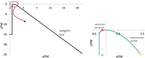
Ogee spillway profile

The smoothness of the geometry at the weir profile greatly affects the pressure distribution along the spillway. Small deviations in the radius of curvature may cause significant local pressure disturbances (Hager, 1987). A widely used ogee crest profile, originating from the Waterways Experiment Station (WES) standard design, is reported by the Corps of Engineers (1970) (USBR, 1987).

The geometry of the ogee spillway consists of various parts. All quantities are made dimensionless with the design head, $H_d$. The upstream quadrant is where the subcritical flow converts to supercritical (Savage & Johnson, 2001). According to the Corps of Engineers (1977), it is usually designed with three arcs of circle with the radius of $0.04H_d$, $0.2H_d$ and $0.5H_d$, respectively (Hager, 1987). (4) $\begin{array}{rl}& {\left(\frac{x}{H_d}+0.2418\right)}^2+{\left(\frac{z}{H_d}+0.1360\right)}^2=(0.04{)}^2\\ & -0.2818\le \frac{x}{H_d}\le -0.2760\end{array}$(4) (5) $\begin{array}{rl}& {\left(\frac{x}{H_d}+0.1050\right)}^2+{\left(\frac{z}{H_d}+0.2190\right)}^2=(0.20{)}^2\\ & -0.276\le \frac{x}{H_d}\le -0.175\end{array}$(5) (6) $\begin{array}{rl}& {\left(\frac{x}{H_d}\right)}^2+{\left(\frac{z}{H_d}+0.5000\right)}^2=(0.50{)}^2\\ & -0.175\le \frac{x}{H_d}\le 0\end{array}$(6)

The downstream section from the crest apex to the tangent line has been reported as a power-law equation (Savage & Johnson, 2001): (7) $\frac{z}{H_d}=-0.5{\left(\frac{x}{H_d}\right)}^{1.85}$(7) where $x$ and $z$ are the stream-wise and upward directions in the Cartesian coordinates system.

The downstream quadrant is followed by a chute tangent line. The origin of coordinates is set on the apex of the crest. The ogee profile of the present study is illustrated in Figure 1.

Figure 1. The ogee spillway and crest profile.

Herein, the spillway design head was set to 15 cm. The slope of the chute is derived to 51 degrees (Peltier et al., 2018). The reservoir and chute are considered long enough to make boundaries far away from the study area and avoid any unwanted effect on ogee crest simulation.

Boundary conditions and computational domain

There are various boundary conditions employed in this study, which are illustrated in Figure 2: (i) two different inlet boundary conditions that were needed to describe the water and air flow separately; (ii) the atmosphere boundary at the upper part of the domain above the air phase; (iii) right boundary which is defined as the flow outlet; and (iv) the lower wall, which is the bottom of the reservoir, the spillway and the channel bed. Note that this case is solved in 2 dimensions vertically (2DV). Since ogee spillways have a free wide crest, wall effects do not reach to the centerline, and vertical 2-dimensional modeling does not limit the result significantly.

Figure 2. Solution domain and boundaries in ogee spillway simulation.

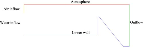
The inlet patch was divided into water-inlet and air-inlet boundaries. The boundary condition at the entrance patch of the flow domain was set as the known velocity boundary. The stream-wise water velocity in the inlet was set in a way so that water surface elevation was in accordance with the specific hydraulic head ratio in each case. For other parameters, a fixed value boundary condition is set in the inlet patch.

The boundary conditions at the lower wall boundary were specified as no-slip. The standard wall function is used for the boundary conditions for other parameters in the lower wall patch. A zero gradient boundary condition is defined at the outlet patch in all cases. The so-called inlet–outlet boundary condition was assigned to the upper surface. It is normally the same as the zero-gradient open boundary condition but switches to the fixed-value boundary condition if there is any backward flow.

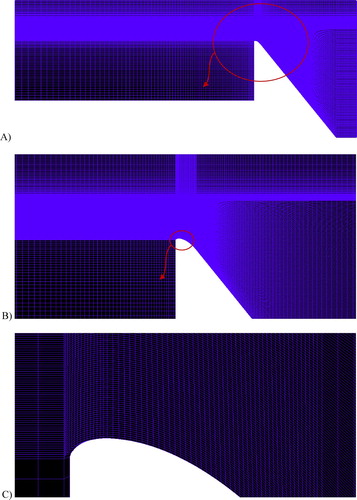
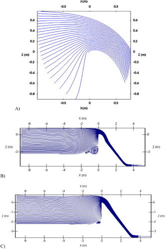
The computational domain is shown in Figure 3. A structured mesh was used to discretize the domain. Because the reservoir in the upstream and downstream channel is quite long, it is computationally very expensive to apply a uniform mesh to the entire domain, so discretization is done with a high resolution at the ogee crest vicinity.

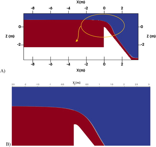
Figure 3. Computational grid (A) overall view (B) closer view (C) vicinity of the crest.

A sensitivity analysis was performed and the developed model was run with three mesh sizes of 3.5, 3 and 2.5 mm. The quantitative data of stream-wise velocity at the top of the ogee crest is presented in Figure 4.

Figure 4. Sensitivity analysis for grid size (A) comparison of velocity result with different mesh size (B) closer view.

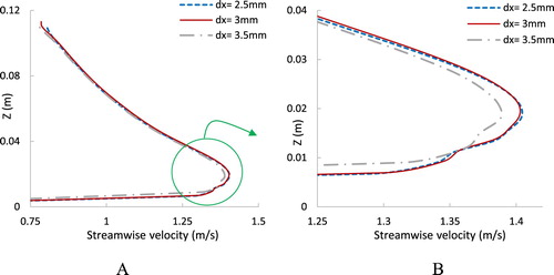
It can be seen that while the mesh size decreases from 3.5 to 3 mm, the velocity results change. This shows that model results are sensitive to the grid size and have not become independent yet.

At the next step, the mesh size was decreased to 2.5 mm. It was found that with decreasing the size of mesh to 2.5 mm, the model results did not show any changes compared with the results of 3 mm grid size. It shows that model results are not dependent on the grid size anymore and have become independent from it. So, it is rational to select coarser mesh size to reduce the computation cost. Therefore, 3 mm was chosen as the grid size of developed numerical model. The final value of mesh in various conditions is almost 185,000 cells.

Numerical algorithm

The governing equations were numerically solved using the interFoam solver in the OpenFOAM framework. The interFoam solver is mostly used for incompressible, isothermal immiscible fluids using a Volume of Fluid (VOF) phase-fraction-based interface-capturing approach. In VOF method, the tracking of the interface between the phases is accomplished by the solution of a continuity equation for the volume fraction of phases. In addition, the interface between the phases is not calculated explicitly. Then, the phase fraction can have any value between 0 and 1 (Greenshields, 2018). Simulated water and air phase fraction fields and water surface are shown in Figure 5.

Figure 5. Water and air phases in simulated case for head ratio of 5 (A) overall view (B) vicinity of ogee crest.

The finite volume method is implemented in OpenFOAM. It uses different numerical schemes which are applied for space and time discretization.

In the current study, the temporal term was discretized using the Euler scheme. The linear method was used for interpolation schemes. The divergence terms were discretized using the Gauss linear, Gauss vanLeer and Gauss upwind schemes. The Gauss linear scheme was used for the gradient term and Laplacian terms discretization. The Preconditioned Conjugate Gradient (PCG) method and Diagonal Incomplete Cholesky (DIC) pre-conditioner were used for the pressure field with a tolerance of 10⁻⁷. These algorithms had better performance in numerical stability and accuracy compared to others. The start-up water level of the simulation is set to the full reservoir elevation in each case. The default time step interval was set to 0.001 s, but the actual time step was automatically adjusted based on the numerical stability criteria. The results became almost steady after about 10 s of simulation time. To be conservative, all the simulations were run up to 15 s. In all cases, the Courant number was less than 1. Sensitivity analyses showed that a smaller default time step and Courant number did not significantly change the results.

Turbulence models

Little attention has been paid to the simulation of turbulent high-head flows, while it is a delicate issue to select the most suitable turbulence model.

The turbulent-viscosity hypothesis substituted into Equation (3) is (Furbo, 2010): (8) $\begin{array}{rl}\frac{\mathrm{\partial }{\overline{u}}_i}{\mathrm{\partial }\text{t}}+{\overline{u}}_j\frac{\mathrm{\partial }{\overline{u}}_i}{\mathrm{\partial }{\text{x}}_j}& =-\frac{1}{\rho }\frac{\mathrm{\partial }}{\mathrm{\partial }{\text{x}}_i}\left(\overline{p}+\frac{2}{3}\rho k\right)\\ & +\frac{\mathrm{\partial }}{\mathrm{\partial }{\text{x}}_i}\left[\left(\nu +{\nu }_T\right)\left(\frac{\mathrm{\partial }{\overline{u}}_i}{\mathrm{\partial }{\text{x}}_j}+\frac{\mathrm{\partial }{\overline{u}}_j}{\mathrm{\partial }{\text{x}}_i}\right)\right]\end{array}$(8) where $k$ is the turbulent kinetic energy and ${\nu }_T$ is the turbulent viscosity.

Since the Reynolds Averaged Navier–Stokes equations (RANS) simulations are more practical in the field of hydraulic engineering, herein, the simulation of flows over hydraulic structure has been performed using a total of 5 turbulence models: 4 most widely used turbulence models including standard k–ε, RNG k–ε, realizable k–ε, k–ω SST and also LRR, which is usually called a second-order closure and is not categorized in linear eddy viscosity models as in previous ones.

The most commonly used RANS closure model is the standard k–ε model. This model closes the RANS by proposing equations to solve the shear stresses by a linear constitutive relationship.

The following equations are used in standard k–ε turbulence model: (9) $\begin{array}{rl}\frac{\mathrm{\partial }k}{\mathrm{\partial }t}+\frac{\mathrm{\partial }k{u}_i}{\mathrm{\partial }{x}_i}& =\frac{\mathrm{\partial }}{\mathrm{\partial }{x}_i}\left[\left(\nu +\frac{{\nu }_T}{{\sigma }_k}\right)\frac{\mathrm{\partial }k}{\mathrm{\partial }{x}_i}\right]+G_k-\epsilon \end{array}$(9) (10) $\begin{array}{rl}\frac{\mathrm{\partial }\epsilon }{\mathrm{\partial }t}+\frac{\mathrm{\partial }\epsilon u_i}{\mathrm{\partial }{x}_i}& =\frac{\mathrm{\partial }}{\mathrm{\partial }{x}_i}\left[\left(\nu +\frac{{\nu }_T}{{\sigma }_{\epsilon }}\right)\frac{\mathrm{\partial }\epsilon }{\mathrm{\partial }{x}_i}\right]\\ & +C_{1\epsilon }\frac{\epsilon }{k}{G}_k-C_{2\epsilon }\frac{{\epsilon }^2}{k}\end{array}$(10) (11) $\begin{array}{rl}{\nu }_T& =C_{\mu }\frac{k^2}{\epsilon }\end{array}$(11) where $k$ is the turbulent kinetic energy and $\epsilon$ is the rate of turbulent kinetic energy dissipation.

In addition to the k–ε model, some other models are employed to model the turbulence that follow the hypothesis of linear eddy viscosity. The k–ω model uses the turbulence frequency of the large eddies (Farhadi, Mayrhofer, Tritthart, Glas, & Habersack, 2018). The k–ω SST (Shear Stress Transport) model is a variation of the standard k–ω model that computes turbulences when they are far from the local equilibrium. This model also has a good behavior in adverse pressure gradients and separating flow (Lee, 2018). (12) $\begin{array}{rl}\frac{\mathrm{\partial }k}{\mathrm{\partial }t}+u_i\frac{\mathrm{\partial }k}{\mathrm{\partial }{x}_i}& =\frac{\mathrm{\partial }}{\mathrm{\partial }{x}_i}\left[\left(\nu +{\sigma }_k{\nu }_T\right)\frac{\mathrm{\partial }k}{\mathrm{\partial }{x}_i}\right]+P_k-{\beta }^{\ast }k\omega \end{array}$(12) (13) $\begin{array}{rl}\frac{\mathrm{\partial }\omega }{\mathrm{\partial }t}+u_i\frac{\mathrm{\partial }\omega }{\mathrm{\partial }{x}_i}& =\frac{\mathrm{\partial }}{\mathrm{\partial }{x}_i}\left[\left(\nu +{\sigma }_{\omega }{\nu }_T\right)\frac{\mathrm{\partial }\omega }{\mathrm{\partial }{x}_i}\right]+\alpha S^2\\ & -\beta {\omega }^2+2\left(1-F_1\right){\sigma }_{\omega 2}\frac{1}{\omega }\frac{\mathrm{\partial }k}{\mathrm{\partial }{x}_j}\frac{\mathrm{\partial }\omega }{\mathrm{\partial }{x}_j}\end{array}$(13) (14) $\begin{array}{rl}{\nu }_T& =\frac{a_{1}k}{max\left(a_1\omega ,S{F}_2\right)}\end{array}$(14)

The RNG k–ε (Renormalization Group) model employed renormalization group theory to modify the transport equation for ε. (15) $\begin{array}{rl}\frac{\mathrm{\partial }\epsilon }{\mathrm{\partial }t}+\frac{\mathrm{\partial }\epsilon x_i}{\mathrm{\partial }{x}_i}& =\frac{\mathrm{\partial }}{\mathrm{\partial }{x}_i}\left[\left(\nu +\frac{{\nu }_T}{{\sigma }_{\epsilon }}\right)\frac{\mathrm{\partial }\epsilon }{\mathrm{\partial }{x}_i}\right]+C_{1\epsilon }\frac{\epsilon }{k}{G}_k\\ & -\left(C_{2\epsilon }+\frac{C_{\mu }{\eta }^3\left(1-\eta /{\eta }_o\right)}{1+\beta {\eta }^3}\right)\frac{{\epsilon }^2}{k}\end{array}$(15)

In the standard k–ε model, the turbulent viscosity is defined in a way that allows normal turbulent stresses to become negative. The realizable k–ε model exerts some mathematical constraints on the normal stresses to keep them positive, in accordance with their definition (Furbo, 2010). (16) $\begin{array}{rl}\frac{\mathrm{\partial }k}{\mathrm{\partial }t}+\frac{\mathrm{\partial }k{u}_i}{\mathrm{\partial }{x}_i}& =\frac{\mathrm{\partial }}{\mathrm{\partial }{x}_i}\left[\left(\nu +\frac{{\nu }_T}{{\sigma }_k}\right)\frac{\mathrm{\partial }k}{\mathrm{\partial }{x}_i}\right]\\ & +G_k-\epsilon +G_b-Y_M+S_k\end{array}$(16) (17) $\begin{array}{rl}\frac{\mathrm{\partial }\epsilon }{\mathrm{\partial }t}+\frac{\mathrm{\partial }\epsilon u_i}{\mathrm{\partial }{x}_i}& =\frac{\mathrm{\partial }}{\mathrm{\partial }{x}_i}\left[\left(\nu +\frac{{\nu }_T}{{\sigma }_{\epsilon }}\right)\frac{\mathrm{\partial }\epsilon }{\mathrm{\partial }{x}_i}\right]+C_{1\epsilon }\frac{\epsilon }{k}{C}_{3\epsilon }{G}_b\\ & +C_{1}S\epsilon -C_2\frac{{\epsilon }^2}{k+\sqrt{\nu \epsilon }}+S\epsilon \end{array}$(17)

The LRR (Launder-Reece-Rodi) model is one of the variants of the Reynolds Stress Models (RSM) (Greenshields, 2018). It avoids the eddy viscosity approach and determines the turbulent stresses directly by solving six transport equations attained by performing algebra on time-averaged and instantaneous Navier–Stokes equations (Hekmatzadeh, Papari, & Amiri, 2018; Rahimzadeh, Maghsoodi, Sarkardeh, & Tavakkol, 2012). (18) $\begin{array}{rl}& \frac{\mathrm{\partial }}{\mathrm{\partial }\text{t}}\left(\rho \overline{{\acute{u}}_i{\acute{u}}_j}\right)+\frac{\mathrm{\partial }}{\mathrm{\partial }{\text{x}}_k}\left(\rho {\text{u}}_k\overline{{\acute{u}}_i{\acute{u}}_j}\right)\\ & =-\frac{\mathrm{\partial }}{\mathrm{\partial }{\text{x}}_k}\left[\rho \overline{{\acute{u}}_i{\acute{u}}_j{\acute{u}}_k}+\overline{\acute{p}\left({\delta }_{kj}{\acute{\text{u}}}_i+{\delta }_{ki}{\acute{\text{u}}}_j\right)}\right]\\ & +\frac{\mathrm{\partial }}{\mathrm{\partial }{\text{x}}_k}\left[\mu \frac{\mathrm{\partial }}{\mathrm{\partial }{\text{x}}_k}\left(\overline{{\acute{u}}_i{\acute{u}}_j}\right)\right]\\ & -\rho \left(\overline{{\acute{u}}_i{\acute{u}}_j}\frac{\mathrm{\partial }{\text{u}}_j}{\mathrm{\partial }{\text{x}}_k}+\overline{{\acute{u}}_j{\acute{u}}_k}\frac{\mathrm{\partial }{\text{u}}_i}{\mathrm{\partial }{\text{x}}_k}\right)+\overline{\acute{p}\left(\frac{\mathrm{\partial }{\acute{u}}_i}{\mathrm{\partial }{\text{x}}_j}+\frac{\mathrm{\partial }{\acute{u}}_j}{\mathrm{\partial }{\text{x}}_i}\right)}\\ & -2\mu \overline{\frac{\mathrm{\partial }{\acute{u}}_i}{\mathrm{\partial }{\text{x}}_k}\frac{\mathrm{\partial }{\acute{u}}_j}{\mathrm{\partial }{\text{x}}_k}}-2\rho {\mathrm{\Omega }}_k\left(\overline{{\acute{u}}_j{\acute{u}}_m}{ϵ}_{ikm}+\overline{{\acute{u}}_i{\acute{u}}_m}{ϵ}_{jkm}\right)\end{array}$(18)

For further information including turbulence model details and equations, see Pope (2000) and Versteeg and Malalasekera (2007).

Results

Considered case

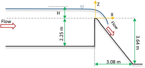
A schematic diagram of the ogee spillway considered in the current study is presented in Figure 6. The spillway follows the above-mentioned geometry. The height of the ogee crest top is 2.25 m from the reservoir bottom. The downstream channel bed is 3.64 m lower than crest apex.

Figure 6. Schematic diagram of the ogee spillway.

The particular aim of this paper is to study the flow over ogee crested spillways under high hydraulic head ratio. To achieve this purpose, the flow hydraulic were investigated at five head ratio ($H/H_d$) values ranging from 1 to 5, by an increment of one. Spillways have the same geometry in all cases.

In this hydraulic conditions, the head, H, was calculated by adding the water depth and the kinetic energy term. (19) $H=h+\frac{U^2}{2g}=h+\frac{Q^2}{2g{B}^2{\left(h+d_{uf}\right)}^2}$(19) where $h$ is the water depth above the crest; $U$ is the discharge velocity; $Q$ is the discharge at the inlet; $B$ is the width of the spillway and $d_{uf}$ is the height of the spillway at the upstream face.

Model evaluation

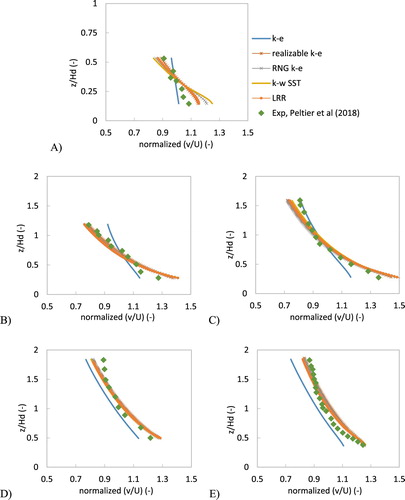
Vertical profiles of computed velocity magnitude at the top of the ogee crest under different head ratio values simulated with various turbulence models are compared with experimental data available in the literature (Peltier et al., 2018) in Figure 7.

Figure 7. Comparison between experimental data (Peltier et al., 2018) and calculated velocities at the top of the ogee crest under different head ratios: (A) $H/H_d=1$; (B) $H/H_d=2$; (C) $H/H_d=3$; (D) $H/H_d=4$; (E) $H/H_d=5$.

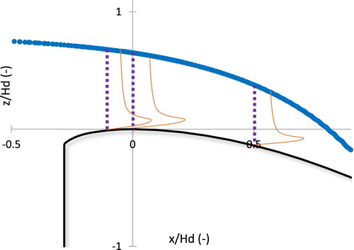
Furthermore, Figure 8 presents a comparison of calculated vertical profiles velocity under high head ratio ($H/H_d=5$) at three locations of slightly before, after and at the apex of ogee crest (indicated in Figure 9).

Figure 8. Comparison between experimental data (Peltier et al., 2018) and calculated velocities under head ratio of 5 at different locations: (A) $x/H_d=-0.1$; (B) $x/H_d=0$; (C) $x/H_d=0.5$.

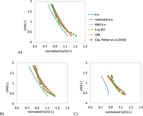
Figure 9. Sketch of positions of velocity profile data.

Figures 7 and 8 indicate that the agreement between measurements and simulations is quite good except for k−ε turbulence model. While, other turbulence models including realizable k–ε, RNG k–ε, k–ω SST and LRR follow the same trend in almost all cases.

To obtain a quantitative measure of the difference between experimental and numerical velocity results, a scatter plot was produced in Figure 10 and various measures of fit were calculated and summarized in Table 1. As shown in Figure 10, most of the simulated velocities were within 10% of the experimental data (Peltier et al., 2018), demonstrating that numerical models can provide reliable results of the flow field over an ogee spillway under high head ratios.

Figure 10. Comparison of the simulated normalized velocity magnitudes obtained by various turbulence models and those from the experimental data (Peltier et al., 2018).

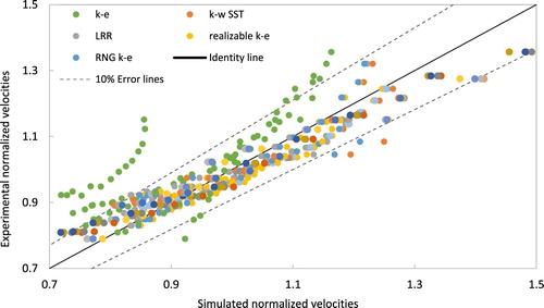
Table 1. Error analysis of calculated vertical profile of velocities on the ogee crest under different head ratios using various turbulence models.

Location	Head ratio	Turbulence model	RMSE	NRMSE	NMSE	R^2	p
$x/H_d=0$	$H/H_d=$1	k–ε	0.04	0.04	0.002	0.94	0.66
		Realizable k–ε	0.05	0.05	0.002	0.94	0.48
		RNG k–ε	0.08	0.07	0.005	0.94	0.51
		k–ω SST	0.09	0.09	0.008	0.93	0.51
		LRR	0.05	0.05	0.003	0.93	0.54
$x/H_d=0$	$H/H_d=2$	k–ε	0.08	0.07	0.006	0.97	0.83
		Realizable k–ε	0.05	0.05	0.002	0.97	0.88
		RNG k–ε	0.06	0.06	0.004	0.96	0.99
		k–ω SST	0.07	0.06	0.004	0.96	0.97
		LRR	0.06	0.06	0.004	0.96	0.94
$x/H_d=0$	$H/H_d=3$	k–ε	0.08	0.07	0.006	0.95	0.66
		Realizable k–ε	0.05	0.05	0.003	0.99	0.98
		RNG k–ε	0.06	0.05	0.003	0.99	0.97
		k–ω SST	0.05	0.05	0.003	0.99	0.78
		LRR	0.06	0.05	0.003	0.99	0.89
$x/H_d=0$	$H/H_d=4$	k–ε	0.07	0.07	0.006	0.95	0.23
		Realizable k–ε	0.04	0.04	0.002	0.97	0.92
		RNG k–ε	0.04	0.04	0.002	0.97	0.97
		k–ω SST	0.04	0.04	0.002	0.97	0.91
		LRR	0.04	0.04	0.002	0.97	0.99
$x/H_d=0$	$H/H_d=5$	k–ε	0.09	0.08	0.008	0.93	0.04
		Realizable k–ε	0.04	0.04	0.002	0.95	0.50
		RNG k–ε	0.04	0.04	0.001	0.96	0.57
		k–ω SST	0.04	0.04	0.001	0.97	0.70
		LRR	0.03	0.03	0.001	0.97	0.75
$x/H_d=-0.1$	$H/H_d=5$	k–ε	0.08	0.07	0.006	0.96	0.14
		Realizable k–ε	0.04	0.04	0.002	0.96	0.76
		RNG k–ε	0.04	0.03	0.001	0.97	0.89
		k–ω SST	0.03	0.03	0.001	0.98	0.99
		LRR	0.03	0.03	0.001	0.98	0.95
$x/H_d=0.5$	$H/H_d=5$	k–ε	0.20	0.20	0.053	0.82	0.00
		Realizable k–ε	0.04	0.04	0.002	0.94	0.84
		RNG k–ε	0.04	0.04	0.002	0.95	0.95
		k–ω SST	0.05	0.05	0.002	0.96	0.88
		LRR	0.05	0.05	0.002	0.96	0.87

Note: RMSE: root mean square error; NRMSE: normalized root mean square error; NMSE: normalized mean square error; R²: R-squared value; p: adjusted p-value of t-test.

A closer look at Figure 10 showed that the LRR, k–ω SST, RNG k–ε and realizable k–ε models provided better matches with the measurements, whereas the color corresponding to the velocities calculated by the k–ε model deviated farther from the line of agreement.

To measure the quality of numerical simulation, some statistical indicators are applied which are: (20) $\begin{array}{rl}\text{RMSE}& =\sqrt{\frac{\sum ^{{\left(v_{\mathrm{e}\mathrm{x}\mathrm{p}}-v_{\mathrm{c}\mathrm{a}\mathrm{l}\mathrm{c}}\right)}^2}}{n}}\end{array}$(20) (21) $\begin{array}{rl}\text{NRMSE}& =\frac{\text{RMSE}}{\text{Max}\left(v_{\exp }\right)+\text{Min}\left(v_{\exp }\right)/2}\end{array}$(21) (22) $\begin{array}{rl}\text{NMSE}& =\frac{\text{RMS}{\text{E}}^2}{\text{Ave}\left(v_{\exp }\right).\text{Ave}\left(v_{\mathrm{c}\mathrm{a}\mathrm{l}\mathrm{c}}\right)}\end{array}$(22)

The results of the error analysis presented in Table 1 suggested that the LRR model performed the best, especially with increasing the head ratio, as the indicators of the errors of its results were smaller and the R² value was larger. Besides, these statistical indicators showed that four turbulence models of realizable k–ε, RNG k–ε, k–ω SST and LRR show the same errors. This confirms that applying these four turbulence models will lead to similar results. At the same time, the k–ε model leads to errors much greater than other turbulence models, and as the head ratio increases, the error rate increases as well.

Moreover, a statistical significance test was performed to determine whether the results obtained by different methods were practically different. Herein, the t-Test is used to test the null hypothesis, $H_0$, that is: the means of two sets of parameters are equal. (23) $H_0:{\mu }_1-{\mu }_2=0$(23) where ${\mu }_1$ is the mean of numerical results and ${\mu }_2$ is the mean of experimental data.

The result of the t-test indicated whether we can reject the null hypothesis; or if it cannot be rejected, it means the null hypothesis should be accepted.

The test compared all possible pairs of results, and the adjusted p-values between the experimental data and numerical results were listed in Table 1, which should be larger than 0.05. Therefore, in almost every case, the null hypothesis is not rejected. And the observed difference between sample means is not convincing enough to say that the average number of simulated velocities and experimental data differ significantly. This essentially means that the comparison between the experimental data and numerical results is logical. So, all the modeled results except for the k–ε model predictions were not found to be statistically different from the experimental data.

For the next step of validation, calculated pressure along the spillway crest under different head ratio modeled with various turbulence models are compared with experimental data available in the literature (Peltier et al., 2018). An error analysis is performed to quantify the comparison between experimental and numerical pressure results, as summarized in Table 2.

Table 2. Error analysis of calculated pressure along the ogee crest centerline under different head ratios using various turbulence models.

Head ratio	Turbulence model	RMSE	NRMSE	NMSE	R^2	p
$H/H_d=1$	k–ε	0.13	0.41	3.43	0.01	0.00
	Realizable k–ε	0.04	0.21	0.60	0.02	0.08
	RNG k–ε	0.03	0.20	0.47	0.00	0.08
	k–ω SST	0.02	0.18	0.26	0.02	0.10
	LRR	0.04	0.22	0.67	0.01	0.07
$H/H_d=2$	k–ε	0.58	0.24	0.52	0.68	0.12
	Realizable k–ε	0.26	0.11	0.06	0.87	0.95
	RNG k–ε	0.26	0.11	0.07	0.87	0.92
	k–ω SST	0.26	0.11	0.07	0.87	0.99
	LRR	0.26	0.11	0.07	0.87	1.00
$H/H_d=3$	k–ε	0.32	0.15	0.12	0.96	0.40
	Realizable k–ε	0.15	0.07	0.02	0.95	0.91
	RNG k–ε	0.14	0.06	0.02	0.96	0.94
	k–ω SST	0.33	0.16	0.12	0.82	0.73
	LRR	0.22	0.10	0.05	0.90	0.88
$H/H_d=4$	k–ε	0.37	0.17	0.10	0.99	0.22
	Realizable k–ε	0.46	0.21	0.21	0.60	0.92
	RNG k–ε	0.50	0.22	0.27	0.63	0.79
	k–ω SST	0.50	0.22	0.24	0.63	0.80
	LRR	0.51	0.23	0.25	0.63	0.90
$H/H_d=5$	k–ε	1.65	0.72	1.10	0.99	0.00
	Realizable k–ε	0.78	0.34	0.40	0.80	0.02
	RNG k–ε	0.75	0.33	0.39	0.79	0.03
	k–ω SST	0.93	0.40	0.51	0.74	0.00
	LRR	0.31	0.14	0.10	0.88	0.91

Based on the statistical indicators in Table 2, although error values for different turbulence models do not follow a similar trend under various head ratios, it is obvious that the traditional k–ε model is not a proper method to simulate these cases. In addition, it can be concluded that, especially with increasing the head ratio, applying the LRR turbulence model is the best approach to simulate flow over ogee crests.

Discussion

As mentioned previously, eddy-viscosity based models like k–ε and k–ω models have significant shortcomings with respect to complex, real-life turbulent flows that are often encountered in engineering applications such as spillways and weirs. Performance of such models is less than satisfactory in the following circumstances: flows with high degrees of anisotropy; significant streamline curvature; flow separation; flows with zones of re-circulation; and flows influenced by mean rotational effects.

RSM turbulence models (like LRR model) were developed to cope with these main limitations of linear eddy viscosity models: the assumption of isotropic fluid. These models obviously have a great advantage over lower-order turbulence models for the flows that the transport of Reynolds stresses plays a significant role. Resolving this issue is accomplished by avoiding the eddy-viscosity hypothesis and by directly computing the individual components of the Reynolds stress tensor. The consideration of fluid anisotropy makes the model well capable of modeling certain flow features such as significant streamline curvature, flow separation and near-wall turbulence in fully developed boundary layer. Applying the LRR closure makes the numerical model more computationally expensive, but this added computational cost is worthwhile in cases dealing with flow separation or significant streamline curvature, where other linear eddy viscosity models do not do a sufficient job.

Turbulence characteristics

The flow field and the contours of the eddy viscosity are shown in Figures 11 and 12, respectively.

Figure 11. Velocity field ($m/s$) of simulated flow over ogee spillway under head ratio of 5 with LRR turbulence model (A) overall view (B) vicinity of ogee crest.

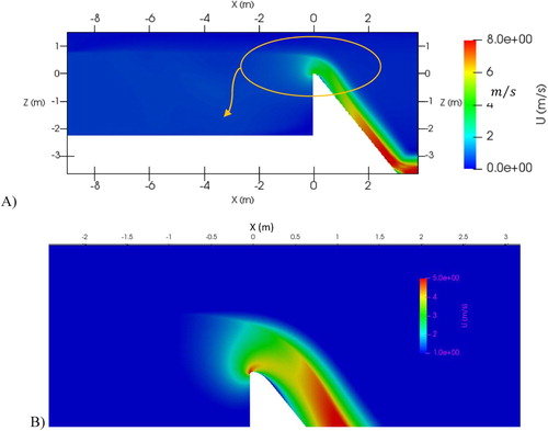
Figure 12. Eddy viscosity ($m^2/s$) contours of simulated flow over ogee spillway under head ratio of 5 with LRR turbulence model.

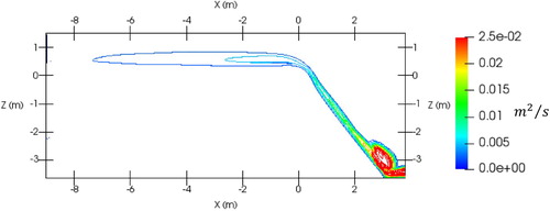
It can be seen from Figure 11 that in the reservoir, velocity is low and flow is not significantly turbulent; except that at the water’s surface of the reservoir, the velocity increases and eddy viscosity grows slowly (see Figure 12).

Passing over the ogee crest and flowing down the slope, velocity increases and consequently a turbulent area develops along the chute as shown in Figures 11 and 12. The areas of high viscosity formed at the downstream of the spillway are identified by the eddy viscosity contours and flow field. The maximum velocity, with a value of 9.4923 $\text{m}/\text{s}$, appears at the toe of the spillway, where the maximum eddy viscosity value of 0.0436 ${\text{m}}^2/\text{s}$ occurs.

Streamlines

For further investigation of the predictive capabilities of the numerical models in simulating the flow field over the ogee crest, the streamlines of flow under head ratio of 5 simulated by the numerical model are shown in Figure 13.

Figure 13. Streamlines of simulated flow over ogee spillway under head ratio of 5 (A) curvature of streamline in the vicinity of ogee crest (B) with LRR model (C) with k–ε model.

Considering that the flow over ogee spillway faces strong flow curvature, the LRR turbulence model is a worthy tool to demonstrate this phenomenon. This points out that the streamlines in the reservoir are mostly parallel; while the flow approaches the ogee crest, the streamlines become concentric and face strong curvature flowing over the spillway. The ability of LRR models in simulating this phenomenon is illustrated in Figure 13. In addition, the rotating flow at the heel of the spillway, which occurs due to no-slip wall resistance, is depicted in Figure 13. It can be seen that the k- ε model shows poor performance in predicting this rotation zone.

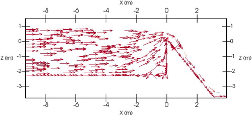
Figure 14 shows the velocity vectors of flow over the ogee spillway using the LRR model under a head ratio of 5. The changes in the direction of velocity vector, from parallel to curvature state, where flow passes over the crest and the rotating area at the corner of the reservoir, are clearly observed in this figure.

Figure 14. Velocity vector of simulated flow over ogee spillway under head ratio of 5 with LRR turbulence model.

Pressure field

In the high head ratio condition, the flow pressure falls below the water vapor pressure along the crest, which leads to negative pressure and the spillway becomes susceptible to cavitation and surface destruction.

In the above-mentioned turbulence models, LRR is the most suitable method to capture this phenomenon.

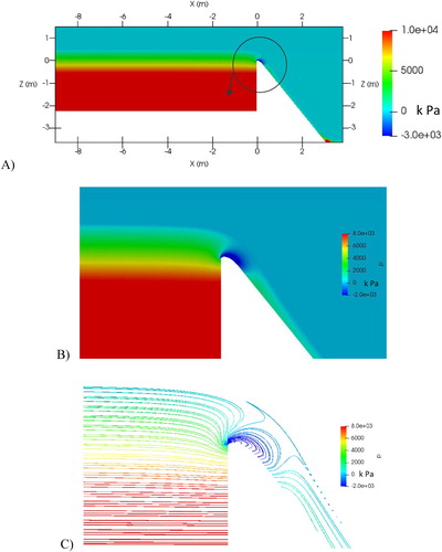
Pressure values over the entire domain and in the vicinity of the ogee crest are illustrated in Figure 15. As seen in Figure 15, a mild negative pressure zone was seen forming over the upstream crest profile in the numerical model with a head ratio of 5. This zone starts from the upstream arc of the ogee crest and stretches along the downstream section.

Figure 15. Pressure domain (kPa) of simulated flow over ogee spillway under head ratio of 5 with LRR turbulence model (A) overall view (B) vicinity of ogee crest (C) pressure contours.

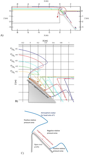
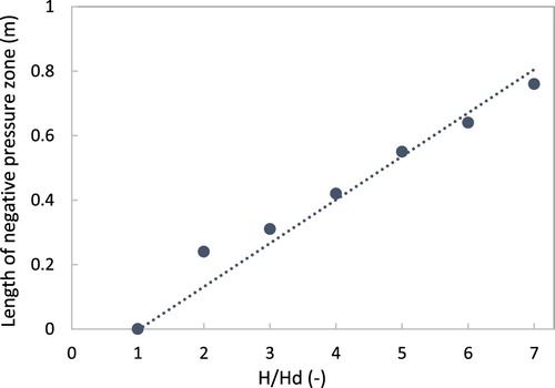
To have a better understanding of how head ratio affects negative pressure flow, the lengths of negative pressure zones computed in various cases are displayed in Figure 16.

Figure 16. Contour of zero relative pressure and negative pressure zone under different head ratio (results of LRR model) (A) overall view (B) closer view.

Since one of the main advantages of the LRR turbulence model is its capability in capturing this negative related pressure zone, all results are calculated by this model.

Figure 16(A) presents the calculated atmospheric isobar curve over the ogee crest profile. Different colors show contours of zero relative pressure for different head ratio.

A closer view of Figure 16(B) shows that it forms an area on the top of the ogee spillway in which relative pressure is negative, while in areas in the upstream and along the chute the pressure is above the atmospheric pressure.

That information is represented on the following schematic (Figure 16(C)), where the zero isobar is illustrated over the ogee crest profile. Also, negative and positive pressure areas and length of negative pressure area are demonstrated on it.

It can be seen from Figure 16(B) that when hydraulic head equals design head, the zero-pressure contour matches the water surface and no negative pressure has occurred, in accordance with expectation.

While the hydraulic head increases and becomes higher than the design head, the pressure dips slightly below water vapor pressure and increases the amplitude of the local negative peak. This strong decrease in pressure can be responsible for cavitation and nappe instabilities (Erpicum et al., 2018).

The length of negative pressure zone versus head ratio is depicted in Figure 17, which shows an ascending linear trend in the size of this zone ($R^2=0.96$).

Figure 17. Length of negative pressure zone versus head ratio (results of LRR model).

Discharge coefficient

The discharge coefficient is a quantitative tool that indicates the spillway efficiency. The discharge coefficient, $C_d$, is an important design parameter of ogee spillways and defined as (Corps of Engineering, 1977): (24) $q=C_d\sqrt{2g}{H}^{1.5}$(24) where $q$ is flow rate per unit width.

The discharge coefficient has a direct relationship with the pressure on the crest. For heads smaller than the design head, there is positive relative pressure over the crest and the discharge coefficient is less, compared to the situation in which the head is equal to the design head. When the head ratio is more than one, the relative pressure on the spillway is negative, resulting in suction and more flow passing over the spillway. This, in turn, causes the discharge coefficient to increase.

Discharge coefficient changes computed by LRR numerical model versus head ratio are depicted in Figure 18.

Figure 18. Discharge coefficient versus head ratio (results of LRR model).

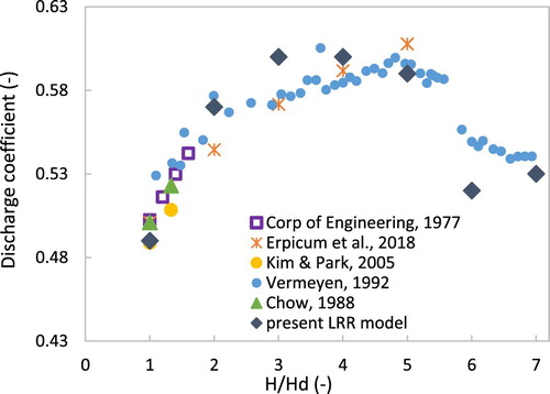
Most data available in the literature has focused on heads near the design head and has shown that generally, discharge coefficients increased with increasing head ratio (Corps of Engineering, 1977; Erpicum et al., 2018; Jafari-Nodoushan et al., 2016; Kim & Park, 2005).

In this paper, high head ratios are investigated and it is shown in Figure 18 that the discharge coefficient increases to a maximum value, it stays constant for some head ratios, then decreases considerably. Almost the same trend was reported by Vermeyen (1992). It could be explained in this way that growing hydraulic head, the water thickness over the ogee spillway increases and the curvature of streamlines reduce gradually. In that phase, the ogee crest tends to operate as a sharp crest and the pressure profile becomes moderately uniform.

To investigate more the reason of a drop in discharge coefficient value for head ratio above 5, the details of streamlines and potential flow detachment over the ogee crest are considered. The streamlines of simulated flow over ogee spillway under the head ratio of 6 are illustrated in Figure 19. The figure focused on the crest to have a better view of probable eddies and flow detachment phenomenon.

Figure 19. Streamlines of simulated flow over ogee spillway under head ratio of 6 (results of LRR model).

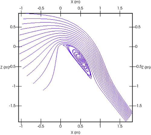
It can be seen from Figure 13(A) that in the case with head ratio equal to 5, while the flow approaches the ogee crest, the streamlines remain parallel to each other and no eddy is formed on the crest. Conversely, when head ratio is increased to 6 (see Figure 19), the flow curvature is no more able to follow up the downstream shape of the spillway. An eddy is formed on the crest and is developed along the downstream side of the spillway. This indicates the flow detachment is occurred on the ogee crest for heads 6 times greater than the design head.

It can be concluded from the simulated results that flow separation on the ogee crest is not occurred for head ratio less than 5, but it will happen for heads more than 6 times of the design head, which is consistent with the literature (Vermeyen, 1992) and observation of Erpicum et al. (2018).

In addition, the specification of the negative pressure zone on the ogee crest is considered to explain the drop in discharge coefficient. Figure 17 shows that the length of negative pressure zone for different head ratios. Moreover, minimum pressure in the negative pressure zone is calculated by numerical model for head ratios of 5 and 6 and presented in Table 3.

Table 3. Specification of the negative pressure zone over ogee crest.

Head ratio	$H/H_d=5$	$H/H_d=6$
Length of negative pressure zone (cm)	55	64
Minimum relative pressure $P_{rel}/H_d$ (–)	−5.9	−1.2

Details presented in Table 3 indicate that although negative pressure zone along the crest in head ratio of 6 is longer than the case of head ratio of 5, the minimum pressure is less negative than for case head ratio of 5. This behavior which is related to the flow detachment explains the drop in discharge coefficient value for head ratio above 5 in the present numerical simulation.

Conclusion

Many researchers have attempted to investigate the hydraulics of ogee crest structure under hydraulic heads near the design head. Herein, an ogee-crested spillway is studied at heads significantly higher than the design head. The efforts are undertaken to study velocity and pressure fields under high head ratio conditions using open-source software, OpenFOAM. The simulated results from a 2DV numerical model with five turbulence closures (standard k–ε, realizable k–ε, RNG k–ε, k–ω SST and LRR) were compared to the experimental data available in the literature.

The main conclusions of the present study are as follows:

• The comparisons of velocity profile and pressure domain over the ogee crest under different head ratios demonstrated that most of the models can provide reliable results of the flow fields over an ogee spillway under high head ratio, but the LRR model had the best performance, especially with increasing the head ratio. The strength of LRR closure is demonstrated in cases dealing with flow separation or significant streamline curvature, which are the limitations of other linear RANS turbulence models.

• The negative pressure zone formed under different high head ratios was examined, and its changes via head ratio were investigated. It was found that when increasing hydraulic head up to seven times that of the design head, the negative pressure zone grew linearly.

• The discharge coefficient as a practical parameter for spillways was studied. Discharge coefficients were calculated according to the results of the numerical model for a wide range of head ratios. It can be concluded that increasing the head ratio up to 5 leads to an increase in the discharge coefficient due to the decrease of the pressure immediately after the separation zone and flow suction. As the head ratio increases to greater values, the discharge coefficient drops suddenly and experiences significantly smaller values due to some changes in the pressure field.

The present research only focuses on the application of different RANS turbulence models in the flows over ogee spillways. Future study can investigate the performance of other advanced turbulence models such as LES.

Disclosure statement

No potential conflict of interest was reported by the authors.

ORCID

Hanifeh Imanian http://orcid.org/0000-0001-5022-1993

Abdolmajid Mohammadian http://orcid.org/0000-0001-5381-8189

References

- Bhajantri, M. R., Eldho, T. I., & Deolalikar, P. B. (2006). Two-dimensional free surface flow over a spillway-a numerical model case study. ISH Journal of Hydraulic Engineering, 12(2), 7–24. doi: 10.1080/09715010.2006.10514828
- Chanel, P. G., & Doering, J. C. (2008). Assessment of spillway modeling using computational fluid dynamics. Canadian Journal of Civil Engineering, 35(12), 1481–1485. doi: 10.1139/L08-094
- Chatila, J., & Tabbara, M. (2004). Computational modeling of flow over an ogee spillway. Computers & Structures, 82, 1805–1812. doi: 10.1016/j.compstruc.2004.04.007
- Chau, K. W., & Jiang, Y. W. (2001). 3D numerical model for Pearl River estuary. Journal of Hydraulic Engineering, 127(1), 72–82. doi: 10.1061/(ASCE)0733-9429(2001)127:1(72)
- Chau, K. W., & Jiang, Y. W. (2004). A three-dimensional pollutant transport model in orthogonal curvilinear and sigma coordinate system for Pearl River estuary. International Journal of Environment and Pollution, 21(2), 188–198. doi: 10.1504/IJEP.2004.004185
- Corps of Engineers. (1977). Hydraulic design criteria. US army engineer waterways experiment station. Retrieved from https://apps.dtic.mil/dtic/tr/fulltext/u2/a092237.pdf
- Erpicum, S., Blancher, B., Vermeulen, J., Peltier, Y., Archambeau, P., Dewals, B., & Pirotton, M. (2018, May). Experimental study of ogee crested weir operation above the design head and influence of the upstream quadrant geometry. 7th international symposium on hydraulic structures, Aachen.
- Farhadi, A., Mayrhofer, A., Tritthart, M., Glas, M., & Habersack, H. (2018). Accuracy and comparison of standard k-ε with two variants of k-ω turbulence models in fluvial applications. Engineering Applications of Computational Fluid Mechanics, 12(1), 216–235. doi: 10.1080/19942060.2017.1393006
- Fleit, G., Baranya, S., & Bihs, H. (2018). CFD modeling of varied flow conditions over an ogee-weir. Periodica Polytechnica Civil Engineering, 2(1), 26–32.
- Furbo, E. (2010). Evaluation of RANS turbulence models for flow problems with significant impact of boundary layers (master's thesis). Uppsala University, Uppsala.
- Greenshields, C. J. (2018). OpenFoam user guide. Version 6. The OpenFoam Foundation. Retrieved from https://cfd.direct/openfoam/user-guide/
- Hager, W. H. (1987). Continuous crest profile for standard spillway. Journal of Hydraulic Engineering, 113(11), 1453–1457. doi: 10.1061/(ASCE)0733-9429(1987)113:11(1453)
- Hekmatzadeh, A. A., Papari, S., & Amiri, S. M. (2018). Investigation of energy dissipation on various configurations of stepped spillways considering several RANS turbulence models. Iranian Journal of Science and Technology, Transactions of Civil Engineering, 42, 97–109. doi: 10.1007/s40996-017-0085-9
- Holzmann, T. (2017). Mathematics, numerics, derivations and OpenFOAM® (4th ed). Leoben: Holzmann CFD. Retrieved from https://holzmann-cfd.de/publications
- Jafari-Nodoushan, E., Hosseini, K., Shakibaeinia, A., & Mousavi, S. F. (2016). Meshless particle modelling of free surface flow over spillways. Journal of Hydroinformatics, 18(2), 354–370. doi: 10.2166/hydro.2015.096
- Johnsen, M. C., & Savage, B. M. (2006). Physical and numerical comparison of flow over ogee spillway in the presence of tailwater. Journal of Hydraulic Engineering, 132(12), 1353–1357. doi: 10.1061/(ASCE)0733-9429(2006)132:12(1353)
- Kanyabujinja, P. N. (2015). CFD modelling of ogee spillway hydraulics and comparison with physical model tests (master's thesis). Stellenbosch University, Stellenbosch.
- Kim, D. G., & Park, J. H. (2005). Analysis of flow structure over ogee-spillway in consideration of scale and roughness effects by using CFD model. KSCE Journal of Civil Engineering, 9(2), 161–169. doi: 10.1007/BF02829067
- Lee, C. (2018). Rough boundary treatment method for the shear stress transport k-ω model. Engineering Applications of Computational Fluid Mechanics, 12(1), 261–269. doi: 10.1080/19942060.2017.1410497
- Peltier, Y., Dewals, B., Archambeau, P., Pirotton, M., & Erpicum, S. (2018). Pressure and velocity on an ogee spillway crest operating at high head ratio: Experimental measurements and validation. Journal of Hydro-Environment Research, 19, 128–136. doi: 10.1016/j.jher.2017.03.002
- Pope, S. B. (2000). Turbulent flows. Cambridge: Cambridge University Press.
- Quezada, M., Tamburrino, A., & Nino, Y. (2018). Numerical simulation of scour around circular piles due to unsteady currents and oscillatory flows. Engineering Applications of Computational Fluid Mechanics, 12(1), 354–374. doi: 10.1080/19942060.2018.1438924
- Rahimzadeh, H., Maghsoodi, R., Sarkardeh, H., & Tavakkol, S. (2012). Simulating flow over circular spillways by using different turbulence models. Engineering Applications of Computational Fluid Mechanics, 6(1), 100–109. doi: 10.1080/19942060.2012.11015406
- Savage, B. M., & Johnson, M. C. (2001). Flow over ogee spillway: Physical and numerical model case study. Journal of Hydraulic Engineering, 127(8), 640–649. doi: 10.1061/(ASCE)0733-9429(2001)127:8(640)
- Shaheed, R., Mohammadian, A., & Kheirkhah Gildeh, H. (2018). A comparison of standard k–ε and realizable k–ε turbulence models in curved and confluent channels. Environmental Fluid Mechanics, 19(2), 543–568. doi: 10.1007/s10652-018-9637-1
- Turan, C., Carrica, P. M., Lyons, T., Hay, D., & Weber, L. (2008). Study of the free surface flow on an ogee-crested fish bypass. Journal of Hydraulic Engineering, 134(8), 1172–1175. doi: 10.1061/(ASCE)0733-9429(2008)134:8(1172)
- US Department of the interior. Bureau of Reclamation [USBR]. (1987). Design of small dams. Denver (CO).
- US Department of the interior. Bureau of Reclamation [USBR]. (2014). Appurtenant structures for dams (Spillways and outlet works). Design Standards. 14(3). Retrieved from https://www.usbr.gov/tsc/techreferences/designstandards-datacollectionguides/finalds-pdfs/DS14-3.pdf
- Vermeyen, T. B. (1992). Uncontrolled ogee crest research. US Department of the Interior. Bureau of Reclamation. Retrieved from http://www.usbr.gov/pmts/hydraulics_lab/pubs/PAP/PAP-0609.pdf
- Versteeg, H. K., & Malalasekera, W. (2007). An introduction to computational fluid dynamics: The finite volume method. New York, NY: Pearson Education.
- Wu, C. L., & Chau, K. W. (2006). Mathematical model of water quality rehabilitation with rainwater utilization – a case study at Haigang. International Journal of Environment and Pollution, 28(3–4), 534–545. doi: 10.1504/IJEP.2006.011227