Translation simulation of a cylinder in a horizontal pipe

Abstract

This article analyses the passive motion of a cylinder driven by flow in a horizontal pipe using the CFD method. In previous study by Yao et al. (2018) [A new openhole multistage hydraulic fracturing system and the ball plug motion in a horizontal pipe. Journal of Natural Gas Science and Engineering, Vol. 50, pp. 11–21], the motion of a cylinder in a horizontal pipe was investigated experimentally. The cylinder was observed contacting with the pipe bottom, meanwhile it behaved like a guided body with its axis parallel to that of the horizontal pipe. Apart from some observations, it was very hard to gain more knowledge about the flow distribution around the cylinder and the role played by the cylinder's eccentricity in the translation. In order to conduct an extended research, this article concentrates on a general model which considers eccentricity and cylinder–pipe interaction. Moreover, a novel yet efficient approach, which investigates the translation process in a control volume attached to the cylinder, is proposed to simulate the motion utilizing the moving reference frame technique. A series of numerical simulations, with various cylinder dimensions and eccentricities, are conducted to investigate the dynamics of the cylinder and fluid. Meanwhile, the validity of the simulations is proved by comparing the results of experiments with the simulations. Lastly, an error analysis is conducted, and the limitations of this study are highlighted.

Keywords:

• Cylinder
• horizontal pipe
• eccentricity
• translation

1. Introduction

Experiments are limited in terms of systematic and precise measurements. An analytical model for high-speed jet-impinging two-phase flow is difficult to solve precisely. However, the CFD method performs well on a complex flow field, especially in down-hole conditions. Therefore, it was used to investigate the mechanism and characteristics of annular helical flow and its sweeping efficiency on a sandbed.

Numerous engineering applications, ranging from down-hole plug pumping in oil wells to missile launching in a torpedo tube, can be modeled by a cylinder translating with fluid flow in a horizontal pipe. The instantaneous force that acts on the cylinder is often of interest during the translating process (Liu, Bau, & Hu, 2004). This kind of fluid–solid coupling flow is complex because it is inherently transient and affected by several physical parameters (Kartushinsky, Michaelides, Rudi, Tisler, & Shcheglov, 2011). For cylinder-shaped equipment running in a pipeline, the translating process may be affected by the eccentricity, which is characterized by the distance between the axes of the equipment and the pipeline, the equipment's aspect-ratio and equipment–pipeline interaction.

In an preliminary study (Yao, Ding, Hou, Liu, & Zhang, 2018), general pipeline-running equipment was simplified as a cylinder, and experimental means were adopted to investigate the cylinder's motion. In the experiments, terminal velocities of a certain number of cylinders under different flow rates were measured. Although the experiments were able to provide some useful practical/engineering information, they could provide hardly any knowledge about the flow around the cylinder. As for the theoretical method, the broad-ends of a cylinder make it hard to predict the flow precisely, especially when the cylinder's aspect-ratio is not large enough. Worse still, the role that eccentricity played in the experiments was not clear because it was challenging to adjust eccentricity without introducing adverse side effects. Meanwhile, the Computational Fluid Dynamics (CFD) method has a good performance (Ghalandari, Koohshahi, Mohamadian, Shamshirband, & Chau, 2018; Song, Li, Huang, Tian, & Shi, 2011). Therefore, in this article CFD is adopted to fetch more features of the flow, and it is also beneficial for a better understanding of the phenomena observed in the experiments.

In recent years, a number of numerical studies have been published focusing on investigating moving objects in a pipe, and these simulations were conducted either on a mesh or without a mesh.

In the meshed category, most of the simulations were performed with the Eulerian–Lagrange approach (Kartushinsky et al., 2011), whereas other simulations were operated using the Euler–Euler approach. A number of numerical studies published in recent years focus on multiphase flows in confined flow domains. They are performed mostly within the framework of Eulerian–Lagrange simulations. In the Euler–Euler approach, the dispersed object is generalized as a continuum, which is mutually interacting and able to penetrate the primary fluid. It also formulates two approaches with different treatments of the new continua – either a fluid or a material cloud (Göz, Sommerfeld, & Laín, 2006; Ishii & Hibiki, 2011; Reeks, 1993; Zaichik, 1997).

In the Eulerian–Lagrange approach, the flow field is obtained by calculating the Navier–Stokes (N-S) equation in the Euler frame, whereas every dispersed object is tracked with the Lagrangian approach by solving Newton's dynamic equation (Göz et al., 2006). To capture the total dynamic force applied on the object, the instantaneous surface of the object should be determined accordingly. There are also two specific methods to treat the moving surface. The first is the non-geometry-conforming grid method wherein the solid–fluid domain is computed with a fixed and uniform mesh to avoid frequent re-meshing, which is usually called the ‘fictitious domain method’ (Uhlmann, 2005; Uhlmann & Dušek, 2014). The second uses a dynamic fluid domain, subject to the no-slip condition at interfaces with solid objects (Uhlmann, 2005). In FLUENT® (Andy's, Inc. Canonsburg, PA, USA), it is called the dynamic mesh technique and it is widely used in the simulation of particle motion in pipes. It can be used to simulate the falling of a cylinder in a vertical tube (Schaschke, 2010), or to investigate the piston effect of a train in subway tunnel (Kim & Kim, 2007, 2009; López González, Galdo Vega, Fernández Oro, & Blanco Marigorta, 2014; Xue, You, Chao, & Ye, 2014).

In the mesh-free category, taking the Smoothed Particle Hydrodynamics (SPH) method for example (Sun, Sakai, & Yamada, 2013), both the fluid and the solid are tracked by the Lagrangian method and the particles carry the physical properties of a fluid. This method is promising in solving complex flow problems wherein both the fluid–particle interaction and free surface tracking are important (Nestor & Quinlan, 2010; Sun et al., 2013).

In this article, the cylinder translation in a horizontal pipe is simulated. As the cylinder is one single large particle, the dynamic mesh technique is an option for studying the cylinder translation at first sight. However, the simulation can be conducted in a simpler way if one takes the following experimental phenomena into consideration. Firstly, the pipe is very long compared with the cylinder. Secondly, the cylinder translates like a guided body.

Based on the first phenomenon, one is able to select a satellite Control Volume (CV) which is long enough to enclose the cylinder, and the velocity profile on the side-faces of the CV cannot feel the cylinder's existence. Based on the second phenomenon, the cylinder's freedom could be downgraded to 1. With these two simplifications, it is more desirable to conduct the simulation in a moving reference frame which is fixed on the cylinder, because the explicit mesh updating process could be canceled. The boundary condition of the CV could be determined by flow rate and the translating of cylinder. In FLUENT®, this can be done by the Moving Reference Frame (MRF) technique, which provides the built-in infrastructure to the transformation between the absolute laboratory frame and a moving frame.

Rather than specifying the cylinder a prescribed velocity, we are more interested in the case where the cylinder-tube interaction is given to calculate the kinematic of the cylinder and forces acting on it. As well as the present model, the accompanying analyses and computations will be beneficial to scientists and engineers who model the same/similar flows in horizontal pipes/channels.

2. Theoretical basis for this study

2.1. Simplified model for the physical problem

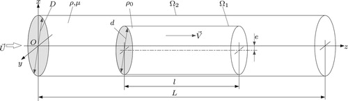
As concluded in previous study (Yao et al., 2018), a heavy cylinder driven by pipe flow will finally reach a terminal velocity with its bottom contacting with that of the pipe. Therefore, we could construct a model where a cylinder is in one-degree-of-freedom translation to depict the original problem, as shown in Figure 1. This problem is generalized from the cylinder–pipe contact case so that the eccentricity coefficient $\epsilon =2e/(D-d)$ could vary in [0,1], where e is the eccentricity, and D, d are the diameters of the pipe and cylinder, respectively. This simple model could describe many engineering practice such as cylinder-shaped deceives running in pipeline, and they are supported by thin legs whose disturbance on fluid is negligible. The length of pipe L is much larger than the cylinder's (l). Both of fluid and cylinder are incompressible continuum with density of ρ and ${\rho }_0$, respectively. Furthermore, the fluid is considered as homogeneous and isotropic with a constant viscosity of μ. $\overrightarrow{U}$ with norm U characterizes pipe flow rate and $\overrightarrow{V}$ with norm V features cylinder's translation velocity. Two dimensionless parameters defined as $\kappa =d/D$ and $\varphi =l/d$ are used to further characterize the physical model.

Figure 1. Schematic diagram of a cylinder translating in a horizontal pipe.

2.2. The fluid governing equations

The basis underlying MRF method is the equivalent description of governing equations in different reference frame, which is a necessary result of physical principle to be independent of the chosen reference frame. In a system that motion would be expressed in different reference frame, it is necessary to handle the motion transformation properly. In the following text, two expressions of a general motion in different frame are coupled by the Galileo transformation, and then the specification in our case is deduced.

Suppose that there is a fixed laboratory reference frame o–123, and the other frame $o^{\prime }$–$1^{\prime }{2}^{\prime }{3}^{\prime }$ moves and rotates relative to o–123, as shown in Figure 2. At an arbitrary time, the origin $o^{\prime }$ of $o^{\prime }$–$1^{\prime }{2}^{\prime }{3}^{\prime }$ is denoted by ${\overrightarrow{r}}_{o{o}^{\prime }}$, meanwhile, the translation and rotation velocity are ${\overrightarrow{u}}_{o{o}^{\prime }}$ and $\overrightarrow{\omega }$. Now, there is a mass point, represented by p, whose position is ${\overrightarrow{r}}_{op}$ in o–123 and ${\overrightarrow{r}}_{o^{\prime }p}$ in $o^{\prime }$–$1^{\prime }{2}^{\prime }{3}^{\prime }$. The velocity of p is expressed by ${\overrightarrow{u}}_{op}$ in o–123 and ${\overrightarrow{u}}_{o^{\prime }p}$ in $o^{\prime }$–$1^{\prime }{2}^{\prime }{3}^{\prime }$.

Figure 2. The motion of a mass point expressed in different frames.

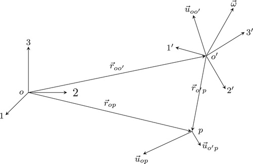
The velocities of p viewed in the two frames can be transformed to each other according to the following equation (1) ${\overrightarrow{u}}_{o^{\prime }p}={\overrightarrow{u}}_{op}-{\overrightarrow{u}}_l,$(1) where ${\overrightarrow{u}}_l$ is the linked velocity of the point fixed in the $o^{\prime }-1^{\prime }{2}^{\prime }{3}^{\prime }$ frame that coincides with p instantaneously, and ${\overrightarrow{u}}_l$ could be derived with the following equation (2) ${\overrightarrow{u}}_l={\overrightarrow{u}}_{o{o}^{\prime }}+\overrightarrow{\omega }\times {\overrightarrow{r}}_{o^{\prime }p}.$(2)

The governing equation of fluid is usually expressed in laboratory system. In system o−123, taking ${\overrightarrow{u}}_{op}$ as the independent variable to describe the motion of a flow element, the mass conservation equation for incompressible fluid with density ρ can be written as (3) $\mathrm{\nabla }\cdot {\overrightarrow{u}}_{op}=0,$(3) and the momentum equation can be written as (4) $\rho \frac{\mathrm{D}{\overrightarrow{u}}_{op}}{\mathrm{D}t}=-\mathrm{\nabla }p+\rho \overrightarrow{g}+\mu {\mathrm{\nabla }}^2{\overrightarrow{u}}_{op},$(4) where $\mathrm{D}/\mathrm{D}t$ is the material deviation.

As Equation (3(3) $\mathrm{\nabla }\cdot {\overrightarrow{u}}_{op}=0,$(3) ) is scalar, it is straightforward that it has the same form in system $o^{\prime }$–$1^{\prime }{2}^{\prime }{3}^{\prime }$ because a scalar is invariant in the transformation of coordinate system, therefore one has (5) ${\mathrm{\nabla }}^{\prime }\cdot {\overrightarrow{u}}_{op}=0\cdot$(5)

Combining Equations (1(1) ${\overrightarrow{u}}_{o^{\prime }p}={\overrightarrow{u}}_{op}-{\overrightarrow{u}}_l,$(1) ), (2(2) ${\overrightarrow{u}}_l={\overrightarrow{u}}_{o{o}^{\prime }}+\overrightarrow{\omega }\times {\overrightarrow{r}}_{o^{\prime }p}.$(2) ) and (5(5) ${\mathrm{\nabla }}^{\prime }\cdot {\overrightarrow{u}}_{op}=0\cdot$(5) ), one gets (6) ${\mathrm{\nabla }}^{\prime }\cdot {\overrightarrow{u}}_{o^{\prime }p}=0$(6) with ${\mathrm{\nabla }}^{\prime }\cdot (\overrightarrow{\omega }\times {\overrightarrow{r}}_{o^{\prime }p})\equiv 0$.

The acceleration of point p in the laboratory system and the moving reference frame has the following relationship: (7) ${\overrightarrow{a}}_a={\overrightarrow{a}}_r+{\overrightarrow{a}}_l+{\overrightarrow{a}}_c,$(7) where ${\overrightarrow{a}}_a$ is the acceleration viewed in the laboratory frame and is in accordance with $\mathrm{D}{\overrightarrow{u}}_{op}/\mathrm{D}t$ in the left-hand-side term in Equation (4(4) $\rho \frac{\mathrm{D}{\overrightarrow{u}}_{op}}{\mathrm{D}t}=-\mathrm{\nabla }p+\rho \overrightarrow{g}+\mu {\mathrm{\nabla }}^2{\overrightarrow{u}}_{op},$(4) ). ${\overrightarrow{a}}_r$ is the relative acceleration in the moving reference frame and ${\overrightarrow{a}}_r=\mathrm{D}{\overrightarrow{u}}_{o^{\prime }p}/\mathrm{D}t$. ${\overrightarrow{a}}_l$ is the link acceleration and ${\overrightarrow{a}}_l=\mathrm{D}\overrightarrow{\omega }/\mathrm{D}t\times {\overrightarrow{r}}_{o{}^{\prime }p}+\overrightarrow{\omega }\times (\overrightarrow{\omega }\times {\overrightarrow{r}}_{o{}^{\prime }p})+\mathrm{D}{\overrightarrow{u}}_{oo{}^{\prime }}/\mathrm{D}t$. ${\overrightarrow{a}}_c$ is Coriolis acceleration and ${\overrightarrow{a}}_c=2\overrightarrow{\omega }\times {\overrightarrow{u}}_{o{}^{\prime }p}$. The partial term of ${\mathrm{\nabla }}^2{\overrightarrow{u}}_{op}$ on the right-hand-side of Equation (4(4) $\rho \frac{\mathrm{D}{\overrightarrow{u}}_{op}}{\mathrm{D}t}=-\mathrm{\nabla }p+\rho \overrightarrow{g}+\mu {\mathrm{\nabla }}^2{\overrightarrow{u}}_{op},$(4) )), combine it with Equations (1(1) ${\overrightarrow{u}}_{o^{\prime }p}={\overrightarrow{u}}_{op}-{\overrightarrow{u}}_l,$(1) ) and (2(2) ${\overrightarrow{u}}_l={\overrightarrow{u}}_{o{o}^{\prime }}+\overrightarrow{\omega }\times {\overrightarrow{r}}_{o^{\prime }p}.$(2) ) one gets (8) ${\mathrm{\nabla }}^2{\overrightarrow{u}}_{op}={\mathrm{\nabla }}^2{\overrightarrow{u}}_{o^{\prime }p}.$(8)

Again, considering the invariance of Laplace operator in the transformation of coordinate system we have (9) ${\mathrm{\nabla }}^2{\overrightarrow{u}}_{o^{\prime }p}={\mathrm{\nabla }}^{\prime 2}{\overrightarrow{u}}_{o^{\prime }p},$(9) thus (10) ${\mathrm{\nabla }}^2{\overrightarrow{u}}_{op}={\mathrm{\nabla }}^{\prime 2}{\overrightarrow{u}}_{o^{\prime }p}.$(10)

Combining Equations (4(4) $\rho \frac{\mathrm{D}{\overrightarrow{u}}_{op}}{\mathrm{D}t}=-\mathrm{\nabla }p+\rho \overrightarrow{g}+\mu {\mathrm{\nabla }}^2{\overrightarrow{u}}_{op},$(4) ), (7(7) ${\overrightarrow{a}}_a={\overrightarrow{a}}_r+{\overrightarrow{a}}_l+{\overrightarrow{a}}_c,$(7) ) and (10(10) ${\mathrm{\nabla }}^2{\overrightarrow{u}}_{op}={\mathrm{\nabla }}^{\prime 2}{\overrightarrow{u}}_{o^{\prime }p}.$(10) ), we can derive the momentum equation in the moving reference frame: (11) $\begin{array}{rl}\rho \frac{\mathrm{D}{\overrightarrow{u}}_{o{}^{\prime }p}}{\mathrm{D}t}& =-\mathrm{\nabla }{}^{\prime }p+\rho \overrightarrow{g}+\mu \mathrm{\nabla }{{}^{\prime }}^2{\overrightarrow{u}}_{o{}^{\prime }p}-\rho \left[\frac{\mathrm{D}\overrightarrow{\omega }}{\mathrm{D}t}\times {\overrightarrow{r}}_{o{}^{\prime }p}\right.\\ & +\left.\overrightarrow{\omega }\times (\overrightarrow{\omega }\times {\overrightarrow{r}}_{o{}^{\prime }p})+\frac{\mathrm{D}{\overrightarrow{u}}_{oo{}^{\prime }}}{\mathrm{D}t}+2\overrightarrow{\omega }\times {\overrightarrow{u}}_{o{}^{\prime }p}\right].\end{array}$(11)

In this article, the moving reference frame is fixed on the cylinder. As mentioned above, the cylinder is in one-degree of freedom translation, so Equation (11(11) $\begin{array}{rl}\rho \frac{\mathrm{D}{\overrightarrow{u}}_{o{}^{\prime }p}}{\mathrm{D}t}& =-\mathrm{\nabla }{}^{\prime }p+\rho \overrightarrow{g}+\mu \mathrm{\nabla }{{}^{\prime }}^2{\overrightarrow{u}}_{o{}^{\prime }p}-\rho \left[\frac{\mathrm{D}\overrightarrow{\omega }}{\mathrm{D}t}\times {\overrightarrow{r}}_{o{}^{\prime }p}\right.\\ & +\left.\overrightarrow{\omega }\times (\overrightarrow{\omega }\times {\overrightarrow{r}}_{o{}^{\prime }p})+\frac{\mathrm{D}{\overrightarrow{u}}_{oo{}^{\prime }}}{\mathrm{D}t}+2\overrightarrow{\omega }\times {\overrightarrow{u}}_{o{}^{\prime }p}\right].\end{array}$(11) ) can be readily simplified with $\overrightarrow{\omega }\equiv \overrightarrow{0}$ such that (12) $\rho \frac{\mathrm{D}{\overrightarrow{u}}_{o{}^{\prime }p}}{\mathrm{D}t}=-\mathrm{\nabla }{}^{\prime }p+\rho \overrightarrow{g}+\mu \mathrm{\nabla }{{}^{\prime }}^2{\overrightarrow{u}}_{o{}^{\prime }p}-\rho \frac{\mathrm{D}{\overrightarrow{u}}_{oo{}^{\prime }}}{\mathrm{D}t}.$(12)

Equations (6(6) ${\mathrm{\nabla }}^{\prime }\cdot {\overrightarrow{u}}_{o^{\prime }p}=0$(6) ) and (12(12) $\rho \frac{\mathrm{D}{\overrightarrow{u}}_{o{}^{\prime }p}}{\mathrm{D}t}=-\mathrm{\nabla }{}^{\prime }p+\rho \overrightarrow{g}+\mu \mathrm{\nabla }{{}^{\prime }}^2{\overrightarrow{u}}_{o{}^{\prime }p}-\rho \frac{\mathrm{D}{\overrightarrow{u}}_{oo{}^{\prime }}}{\mathrm{D}t}.$(12) ) are the conservation equations that govern the motion of fluid observed in the moving reference frame. It is worth noting that the term $-\rho \mathrm{D}{\overrightarrow{u}}_{oo{}^{\prime }}/\mathrm{D}t$ contains ${\overrightarrow{u}}_{oo{}^{\prime }}$, which means that, to close the flow governing equation, the modeling of the instantaneous cylinder translation in the laboratory frame cannot be eliminated.

2.3. The cylinder governing equations

The cylinder motion obeys Newton's dynamic equations. In general, there are three kinds of force acting on the cylinder, as shown in Figure 3.

Figure 3. Schematic diagram of the force applied on a cylinder.

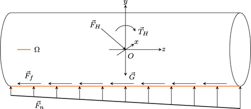
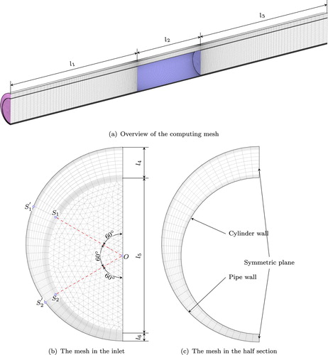
Figure 4. Schematic diagram of the computing mesh (a case of $\kappa =0.8$, $\varphi =3$, $\epsilon =0.6$ in point).

The first is the hydraulic force acting on the surface of the cylinder. This force accounts for the combined effect of the local mean field and the fluctuating turbulence component around the cylinder. This force is not prescribed but run-time calculated. Luckily, FLUENT® provides some macros to allow users to fetch surface force from the solver. So, the influence of hydraulic force could be equalized by net force ${\overrightarrow{F}}_H$ acting on the cylinder centroid O with a resulting torque ${\overrightarrow{T}}_H$.

The second is gravity $\overrightarrow{G}$, which applies at the center of gravity. In this article, the cylinder is treated as homogeneous, so the center of gravity coincides with O.

The third is the interaction between the pipe wall and the cylinder. It is usual practice for cylinder-like robots to use wheeled ‘legs’ across the body to support themselves in the pipeline, so one useful model assumes a linear interaction profile along the bottom line of the cylinder, as depicted in Figure 3. The interaction can be decomposed into a friction force ${\overrightarrow{F}}_f$ and a supporting force ${\overrightarrow{F}}_n$, whose intensity at the left-hand-side and right-hand-side ends of the cylinder could be characterized by $f_1$ and $f_2$, respectively. Hence, one can get ${\overrightarrow{F}}_n=l(f_1+f_2)/2$. Here, an interaction coefficient f between the cylinder and the pipe wall is defined. It could be seen as a generalization of the friction coefficient used when the cylinder contacts the pipe wall. Then, ${\overrightarrow{F}}_f$ and ${\overrightarrow{F}}_n$ are related by ${\overrightarrow{F}}_f=f{\overrightarrow{F}}_n$.

According to the equilibrium equation, one has (13a) $\begin{array}{rl}{\overrightarrow{F}}_H+\overrightarrow{G}+{\overrightarrow{F}}_f+{\overrightarrow{F}}_n+{\overrightarrow{F}}_i& =\overrightarrow{0},\end{array}$(13a) (13b) $\begin{array}{rl}{\overrightarrow{T}}_H+{\overrightarrow{T}}_G+{\overrightarrow{T}}_f+{\overrightarrow{T}}_n+{\overrightarrow{T}}_i& =\overrightarrow{0},\end{array}$(13b) where ${\overrightarrow{F}}_i$ and ${\overrightarrow{T}}_i$ are the inertia force and torque acting on the cylinder; ${\overrightarrow{T}}_G$, ${\overrightarrow{T}}_f$ and ${\overrightarrow{T}}_n$ are the torques produced by gravity, supporting and friction forces with respect to point O. If O is the centroid, one can get (14) ${\overrightarrow{T}}_G=\overrightarrow{0}.$(14)

From the linear interaction assumption, one can get (15a) $\begin{array}{rl}[{\overrightarrow{T}}_f{]}_x& =\frac{ld}{4}(f_1+f_2)f,\end{array}$(15a) (15b) $\begin{array}{rl}[{\overrightarrow{T}}_n{]}_x& =\frac{l^2}{12}(f_1-f_2),\end{array}$(15b) where the subscript x means the vector's x-component.

From force balance in the y-direction and torque balance in the x-direction, one can get (16a) $\begin{array}{rl}{f}_1& =-(6|{\overrightarrow{T}}_H{|}_x+|{\overrightarrow{F}}_H{|}_{y}l-3|{\overrightarrow{F}}_H{|}_{y}fd+mgl-3mgfd)/l^2,\end{array}$(16a) (16b) $\begin{array}{rl}{f}_2& =-(|{\overrightarrow{F}}_H{|}_{y}l-6|{\overrightarrow{T}}_H{|}_x+3|{\overrightarrow{F}}_H{|}_{y}fd+mgl+3mgfd)/l^2,\end{array}$(16b)

Furthermore, from the dynamic equation in the z-direction, the acceleration a of the cylinder can be expressed as (17) $a=|{\overrightarrow{F}}_H{|}_z/m-(f_1+f_2)lf/\left(2m\right).$(17)

The temporal evolution of the cylinder's translation velocity could be solved using Equation (17(17) $a=|{\overrightarrow{F}}_H{|}_z/m-(f_1+f_2)lf/\left(2m\right).$(17) ). The original cylinder motion problem is fully modeled, and the coupled system can be solved using the CFD technique.

3. CFD simulation setup

3.1. Calculating zone and mesh

In Figure 1, the physical domain is symmetric in the xOz plane, wherein the axes of the cylinder and the pipe also lie. The boundary conditions (discussed later) are also symmetric in the xOz plane. Without loss of generality, gravity is considered to be parallel to the xOz plane. Therefore, the mean flow field could be expected to be symmetric accordingly. As a result, a half computational domain, shown in Figure 4(a), is created to investigate the original physical problem. The domain is an internal space of pipe subtracted by that occupied by the cylinder. $l_1$ is the cylinder-inlet distance and $l_3$ is the cylinder-outlet distance. $l_2$ is the length of the cylinder. By trial and error, it is found that $\sum _{i=1}^3{l}_i\sim 5l_2$ is enough to make the simulation results independent of the CV's length. The inlet mesh is shown in Figure 4(b) and the mesh in the half section is shown in Figure 4(c). $l_6$ and $l_4$ are the minimum and maximum gaps between the cylinder and the pipe, respectively. $l_5$ characterizes the cylinder diameter. The left-hand-side face of the domain is assigned an inlet boundary condition where the velocity is uniformly distributed. The right-hand-side face is assigned an outlet boundary condition where the pressure is set to zero (as was done by Ramezanizadeh, Nazari, Ahmadi, & Chau, 2019). The symmetric face of the domain is assigned a symmetric boundary condition. The wall of the pipe and cylinder is assigned the no-slip wall boundary condition.

In order to solve the problem in an economic way, the elements should be dense where the flow gradient is large, and sparse where the flow changes gently. In addition, it is better for the domain to be meshed with structural elements. These features could be achieved by some face manipulation and meshing. Firstly, the end-faces of the cylinder are projected onto that of the pipe along the axial direction, as shown in Figure 4(b). The resulting four end/projection faces are linked and meshed with the same seeding pattern. The triangular cells are used in these end/projection faces and quadrilateral cells are used in the others. A similar operation is applied on the remaining portion of the pipe end-faces. Secondly, the two opposite arcs on the quadrilateral-like face are split with points $S_1$($S_1^{\mathrm{\prime }}$) and $S_2$($S_2^{\mathrm{\prime }}$). As the cylinder gets close to the pipe ($\epsilon \to 1$), the resulting narrow gap can thus be meshed properly by adjusting the mesh transition factor on each arc independently. The edges shown in Figure 4(a) with length $l_i$ $(i=1,2,3)$, and their opposite edges, are linked and meshed with a similar split technique.

These face and edge operations also provide a convenient way to attach boundary layer meshes in the vicinity wall zones. To model viscous effects in a boundary layer accurately, a high-density mesh is required. In the near wall model, there should be at least five mesh layers inside the viscous sub-layer so that the dimensionless wall distance ($y_{\mathrm{w}\mathrm{a}\mathrm{l}\mathrm{l}}^{+}$) is less than one. Here, $y_{\mathrm{w}\mathrm{a}\mathrm{l}\mathrm{l}}^{+}$ and the superscript plus sign are standard in the literature and indicate dimensionless law-of-the-wall variables (see Kundu, Cohen, & Dowling, 2012). For the wall function approach, a sufficient resolution of the boundary layer is also necessary for high quality simulation. On one hand, as shown in Figure 4(c), the boundary layer is attached on the cylinder side wall and pipe wall. On the other hand, the boundary layer can also be formulated along the side face of the cylinder by adjusting the mesh generating factor.

Finally, all of the faces are meshed with triangle or quadrilateral elements, and the computational domain is meshed with the prism elements with a total number of about 302,000.

In the previous experiments, the characteristic Reynolds number was defined by $\mathrm{R}\mathrm{e}=\rho UD/\mu \sim 2\times {10}^4$; therefore, the flow was thought to be turbulent. In this article, the transient 3D N-S equations are solved by a pressure-based solver (which decouples the pressure and velocity fields) in FLUENT®. The time step, which is shared by both the fluid solver and the cylinder motion equation, is set to $1\times {10}^{-4}$ s. It is determined by a trial and error process. Time steps ranging from ${10}^{-6}$ to ${10}^{-3}$ s have been tested, and ${10}^{-4}$ s is a good balance of performance and efficiency. It is short enough to resolve the fluid dynamics and cause no stability or accuracy issues in the calculation. The standard κ–ϵ turbulence model is used for its good performance in predicting highly turbulent pipe flow (Hand, Kelly, & Cashman, 2017). Enhanced Wall Treatment (EWT) is used to treat the near wall flow, as it allows a fine mesh without a deterioration of the results in the zone marked as $l_6$ in Figure 4(b).

In order to model the interactions between the flow and the cylinder, a sub-program, often referred as a ‘User-Defined Function’ (UDF) in FLUENT® (Akaydin, Elvin, & Andreopoulos, 2010), is developed to calculate the motion of the cylinder at every time step and update the boundary conditions for the next fluid solving cycle. The fluid governing equations (6(6) ${\mathrm{\nabla }}^{\prime }\cdot {\overrightarrow{u}}_{o^{\prime }p}=0$(6) ) and (12(12) $\rho \frac{\mathrm{D}{\overrightarrow{u}}_{o{}^{\prime }p}}{\mathrm{D}t}=-\mathrm{\nabla }{}^{\prime }p+\rho \overrightarrow{g}+\mu \mathrm{\nabla }{{}^{\prime }}^2{\overrightarrow{u}}_{o{}^{\prime }p}-\rho \frac{\mathrm{D}{\overrightarrow{u}}_{oo{}^{\prime }}}{\mathrm{D}t}.$(12) ) are solved by the flow solver, and the cylinder motion equation (17(17) $a=|{\overrightarrow{F}}_H{|}_z/m-(f_1+f_2)lf/\left(2m\right).$(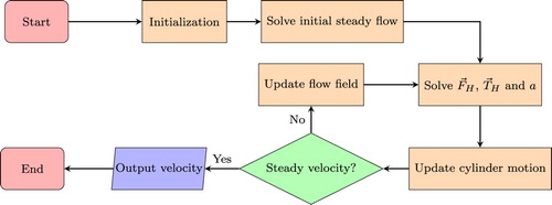17) ) is solved by the UDF, as done by Akaydin et al. (2010), Elvin, Lajnef, Elvin (2006) and Elvin Elvin (2009). The flow chart of this method is shown in Figure 5. A steady initial flow field is solved first as a starting point for the following transient calculation. Then, the calculation switches to an interaction cycle. As the pressure field can be extracted from the fluid solver, ${\overrightarrow{F}}_H$ and ${\overrightarrow{T}}_H$ are readily calculated by surface pressure integration in each calculating cycle; hence, the a in Equation (17(17) $a=|{\overrightarrow{F}}_H{|}_z/m-(f_1+f_2)lf/\left(2m\right).$(17) ) as well as the velocity of the cylinder can be determined. The velocity, pressure of the flow field and the updated cylinder velocity serve as the initial and boundary condition, respectively, for the next calculating cycle until the cylinder is determined to achieve a steady velocity.

Figure 5. Flow chart of the solution of the coupled system.

As stated in the above text, it is clear that the governing equations for the fluid and rigid body domains are solved asynchronously, and the solution data between them are exchanged periodically at every computation cycle (Akaydin et al., 2010). According to Kamakoti and Shyy (2004), this decoupling of the fluid–structure interaction is categorized in the ‘closely coupled’ class, in contrast with the ‘strongly coupled’ class. It is widely used for a good balance of efficiency and robustness in many applications (Kamakoti & Shyy, 2004).

4. Results and discussion

4.1. The cylinder could attain terminal velocity

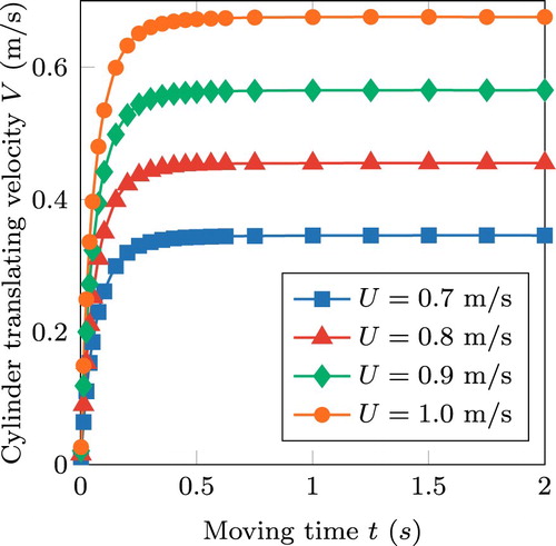
The cylinder will finally reach a constant velocity, $V_t$, which has usually been called the ‘terminal velocity’ in previous research work (Thiessen & Krantz, 1992; Zeng & Schaschke, 2009). Figure 6 shows the transience of the cylinder after releasing. There is a rapid growth of V in the initial stage of moving at a given incoming flow rate U. After that, the V–t curves tend to be flat, which means that $V_t$ has been reached. The shape of V–t curves stay the same but the stable values keep growing as U increases from 0.7 to 1.0 m/s, which means $V_t$ has a positive relationship with U within the scope of this research.

Figure 6. Cylinder transience with cases of $\kappa =0.8$, $\varphi =3$, $\epsilon =0.0$, f = 0.3845 in point.

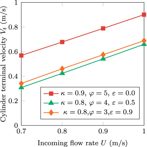
It further reveals the relationship of $V_t$ with U under the effect of some physical parameters, as shown in Figure 7. It is straightforward to deduce that $V_t$ has an obvious linear relationship with U. Additionally, the physical parameters, including κ, ϕ and ϵ, have an impact on the $V_t$–U relationship. Furthermore, for a given cylinder, there exists a $U_i$ to make $V_t/(U-U_i)$ a constant, and this means that the cylinder translation system is self-similar (Zhou, 2013). Therefore, the terminal velocity can be estimated by extrapolation of the linear relationship obtained in this simulation.

Figure 7. The effect of physical parameters on the $V_t$–U relationship.

The simulation results obtained so far also accord with the observations of previous work. Firstly, the existence of a terminal velocity, which is one of the major phenomena observed in the experiment, is reproduced here. Secondly, the linearity of the $V_t$–U relationship complies with the law derived from the experimental data. So, these are two preliminary confirmations of the simulation method, and further validation will be presented in Section 4.4. In the following text, additional flow detail will be extracted from the solver to gain more insight into the flow.

4.2. The effect of eccentricity on the flow field

In a practical/engineering sense, the positional parameters of the cylinder in the pipe are difficult to determine compared with the geometrical parameters. Taking a cylinder-like robot supported by flexible legs in the pipeline, for example, it is hard to measure the orientation of the moving robot with the usual in situ observation equipment because the supporting legs will result in eccentricity, pitch and/or swing of the cylinder. The effect of eccentricity on the flow field and the translation velocity is of special interest and deserves reasonable effort to discover. In the following text, the influence of eccentricity is investigated from the perspective of the flow pattern and streamlines.

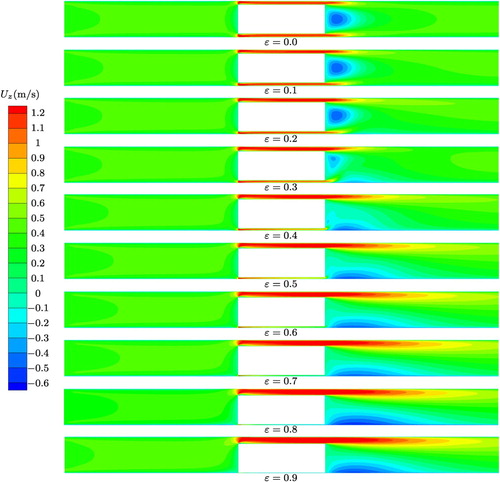
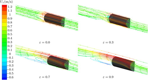
Figure 8 shows the effect of eccentricity on the pattern of $u_z$ (the axial component of the velocity vector) in the plane of symmetry. Here, ϵ varies from 0.0 to 0.9 with a step size of 0.1. In the annular region, the $u_z$ of the pressure driven flow is large at the wide end and small at the narrow end. Thereafter, the annular flow penetrates into the wake zone by convection. It can be seen that the flow pattern is symmetric when the cylinder is concentric with the pipe ($\epsilon =0.0$). Meanwhile, the flow reverses in the wake zone indicating that a vortex ring curls, which is referred to as the ‘original-vortex’ in the following text. The original-vortex is consistent until ϵ reaches 0.3, where it is compressed and distorted. At the same time, a sub-vortex appears below the original-vortex. As ϵ increases from 0.4 to 0.9, the original-vortex gradually collapses, and the sub-vortex stretches and becomes the dominating flow structure.

Figure 8. The effect of eccentricity on the velocity distribution in the half plane (cases of $\kappa =0.8$ and $\varphi =3$ in point).

The streamlines originating from the inlet of the pipe are shown in Figure 9. As $\epsilon =0$, the streamlines shrink and leave the wake zone after passing through the cylinder, which means that the original-vortex can hold itself intact without mass exchange with the outer flow. In other words, a fluid pack is captured by the cylinder to move along with it. Furthermore, the original-vortex must fetch energy from the mean flow through a shear process to balance the inner viscous dissipation. When ϵ reaches 0.3, a few streamlines are captured by the original-vortex to form the complex flow pattern shown in the sub-figure with the same ϵ in Figure 8. Both external energy and momentum are input to the vortex zone through convection. Meanwhile, the streamlines at the bottom are bent up a little as a result of the weak compression effect of the sub-vortex. When ϵ is as large as 0.7 and 0.9, the flow resistance grows considerably near the narrow gap, so a few streamlines are driven upward. It is worth noting that there are some reversed streamlines in the wake zone. The incoming flow participates in the formation of the sub-vortex with length scale that is about the same as the length of the cylinder.

Figure 9. The effect of eccentricity on the stream-trace in the computing zone (with cases of $\kappa =0.8$ and $\varphi =3$ in point).

From the discussion of the flow pattern in the half plane and the streamline distribution around the cylinder, one can safely draw the conclusion that the flow field and the features of the flow structure are dramatically affected by the eccentricity of the cylinder.

4.3. The effect of eccentricity on cylinder terminal velocity

The dynamics of the cylinder are determined by combining the fluid system and the rigid body system. Although the detail of the flow has an apparent relationship with the positional parameter of the cylinder, the terminal velocity of the cylinder, as a result of the overall surface integration of the surface flow variable, is not necessarily influenced by the fluid to such an extent as the detail of the flow.

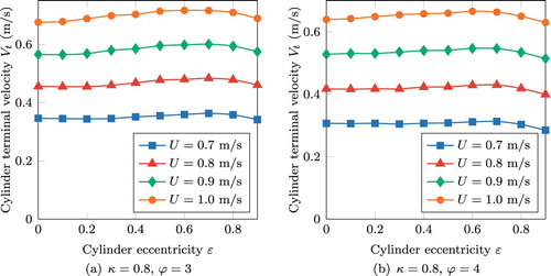
Figure 10 shows the terminal velocity of cylinder at different values of eccentricity. When ϵ increases from 0 to 0.9, the terminal velocity first increases and then decreases a little. It is interesting to note that the curve is convex and the peak velocity is obtained neither in the concentric case nor in the highly eccentric case, but near $\epsilon =0.7$. This accords with the results of the study of Thiessen Krantz (1992) into bimodal terminal velocities using a falling needle viscometer. The difference is that the falling needle will be slow near the wall because of the considerable solid wall shear force. This tendency is independent of the incoming flow velocity. Furthermore, comparing the data in Figure 10(a) where $\varphi =3$ with that in Figure 10(b), this tendency is independent of the cylinder's physical dimensions.

Figure 10. The effect of eccentricity on cylinder terminal velocity.

It is noteworthy that the concentric case is a good approximation of the highly eccentric case. As is well known, the simulation of highly eccentric cases is a challenge because of the wide length scale range. In order to model the whole flow domain, a fine mesh is required in the narrow gap of the annulus, and the resulting number of elements is usually very large. Fortunately, the flow in the narrow gap is usually not of interest. Thus, in some circumstances, it is an effective and time-efficient practice to approximate the motion of a cylinder with any eccentricity using the concentric case without losing much precision. To prove this prospect further, the following study compares simulations of high eccentricity with experiments of full eccentricity.

4.4. Comparison of simulation and experimental results

In the previous study (Yao et al., 2018), the cylinder was observed to lie at the bottom of the pipe, so ϵ should have been one, theoretically. However, some quadrilateral elements in this case have edges of zero length, which is unphysical because it will make the equation discretization invalid. Thus, the simulation results for cases with $\epsilon =0.9$ are used instead.

A series of simulations are carried out. The simulation parameters, including κ, ϕ and f, are the same as those in the experiments. f is very stochastic even when two cylinders have the same nominal roughness on the side surface. So the f in each simulation employs the measured value in the corresponding experiment to eliminate the influence of model-independent factors. Furthermore, the robustness of the simulation will be more evident when it survives the tests wherein the parameter space spans a larger context, just as f does.

Figure 11 shows a comparison of the results of the simulations described in this article and the experimental data. As one can see, most of the experimental data are in the vicinity of simulation lines, i.e. the simulation lines have good predicting performance. Furthermore, the Goodness Of Fit (GOF) $R^2\in (0,1]$, which is usually used to evaluate experimental data fitting quantitatively, is calculated for each comparison group. This is done with the consideration that, if our simulation method is a valid description of the physical problem, the simulation lines should be an effective fitting of the experimental data. As depicted in Figure 11, the GOF varies from 0.8884 to 0.9420, with larger values implying better description.

Figure 11. Numerical and experimental terminal velocities of the cylinder.

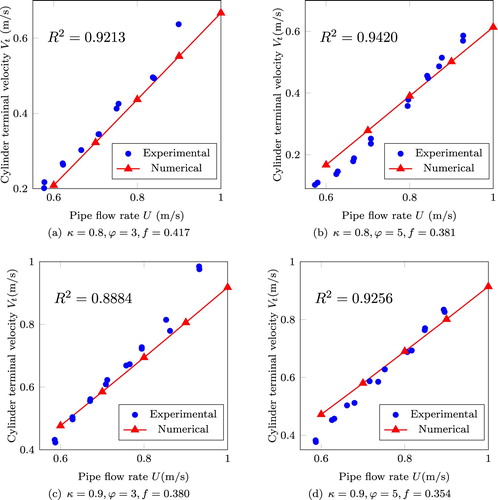
However, it has to be admitted that the experiment data seem to be scattered alongside the simulation line in a non-random manner; in the other words, this implies some systematic errors. Also, some wild data points exist, especially when U is high. Assuming that there are some fitting curves of the experimental data in a least squares sense, they would intersect with the corresponding simulation lines. Furthermore, the former slopes are less than the latter ones – which is where the systematic errors lie. These mismatches could originate from both the modeling process and the conduct of the experiment.

Misinterpretation of the flow may be responsible for errors in the modeling process. For one thing, the standard k–ϵ turbulence model as well as the EWT used to model the fluid may cause errors in resolving the flow around the cylinder. For another, ignorance of a small chamfer of the cylinder will affect the flow pattern. But how these two factors contribute to the systematic error is not yet clear.

As for the experimental procedure, a dimensional analysis has shown that the slope should be determined by κ and ϕ. Because these two parameters can be measured with high precision, not measurement error but ignorance of some other experimental condition could account for the simulation error. These include the unevenness of the pipe/cylinder surface, transience of the incoming flow, system vibration, and so forth. Furthermore, finite stiffness of the mechanical characteristics of the centrifugal pumps is to blame for the larger slope of the fitting lines of the experiment data. In the experiment, flow rate is measured before the cylinder is released; after that, the pump flow rate will rebound a little, which is not taken into consideration in the final determination of the flow rate. As a larger flow rate results in a larger cylinder terminal velocity, the slope of the fitting curve of the experimental data is raised. This phenomenon is more prominent in high-U situations, and it also explains the existence of wild points when U is high.

5. Conclusions

In this article, the simulation of a cylinder translating in a horizontal pipe is conducted. The coupled system is solved by the moving reference frame technique. The flow is solved by the Reynolds-averaged Navier–Stokes method with a turbulence model and the cylinder translation with Newtonian mechanics. Some conclusions can be made, as follows.

• In the simulation, a cylinder could reach terminal velocity after translation, which recasts the experimental phenomena. The terminal velocity varies linearly with the incoming flow rate, and this tendency is independent of the physical properties of the cylinder.

• The flow pattern is strongly dependent on the eccentricity of the cylinder, while the terminal velocity varies a little with the eccentricity. So the terminal velocity attained in the concentric case is a good approximation of that attained in the more highly eccentric case.

• The simulation results accord well with the experimental data obtained in the previous study. The effectiveness and credibility of the simulation and experiment are strengthened by mutual authenticating. Some fluid modeling processes and the conduct of the experiment explain the discepancies found between the simulations and the experimental data.

This study also has limitations. Firstly, the cylinder motion is treated as having strictly one-degree-of-freedom in the proposed method, which limits its application. Secondly, the proposed method is not able to simulate flow where the cylinder is in contact with the pipe wall. Thirdly, the proposed method is not able to simulate the translation of a cylinder in a very short pipe, as the end effects of the pipe cannot be handled properly by the proposed model. In the future, a more capable meshing scheme should be developed to deal with the case where the cylinder is in contact with the pipe. Furthermore, the frozen freedoms of the cylinder in this article should be activated in order to capture more complex translational behavior of a cylinder translating in a horizontal pipe.

Acknowledgments

Consistent help from Mr Tan Quan with writing the manuscript is greatly appreciated.

Disclosure statement

No potential conflict of interest was reported by the authors.

ORCID

Benchun Yao http://orcid.org/0000-0002-2290-0136

Additional information

Funding

This work is supported by the National Natural Science Foundation of China [No. 51509259]; the Fundamental Research Funds for the Central Universities [No. 2462018YJRC017].

References

- Akaydin H. D., Elvin N., & Andreopoulos Y. (2010). Energy harvesting from highly unsteady fluid flows using piezoelectric materials. Journal of Intelligent Material Systems and Structures, 21(13), 1263–1278.
- Elvin N. G., & Elvin A. A. (2009). A general equivalent circuit model for piezoelectric generators. Journal of Intelligent Material Systems and Structures, 20(1), 3–9.
- Elvin N. G., Lajnef N., & Elvin A. A. (2006). Feasibility of structural monitoring with vibration powered sensors. Smart Materials and Structures, 15(4), 977–986.
- Ghalandari M., Koohshahi E. M., Mohamadian F., Shamshirband S., & Chau K. W. (2018). Numerical simulation of nanofluid flow inside a root canal. Engineering Applications of Computational Fluid Mechanics, 13(1), 254–264. doi:10.1080/19942060.2019.1578696
- Göz M. F., Sommerfeld M., & Laín S. (2006). Instabilities in Lagrangian tracking of bubbles and particles in two phase flow. AIChE Journal, 52(2), 469–477.
- Hand B., Kelly G., & Cashman A. (2017). Numerical simulation of a vertical axis wind turbine airfoil experiencing dynamic stall at high Reynolds numbers. Computers and Fluids, 149, 12–30.
- Ishii M., & Hibiki T. (2011). Thermo-fluid dynamics of two-phase flow [Adobe Digital Editions version]. New York: Springer. doi:10.1007/978-1-4419-7985-8
- Kamakoti R., & Shyy W. (2004). Fluid–structure interaction for aeroelastic applications. Progress in Aerospace Sciences, 40(8), 535–558.
- Kartushinsky A. I., Michaelides E. E., Rudi Y. A., Tisler S. V., & Shcheglov I. N. (2011). Numerical simulation of three-dimensional gas–solid particle flow in a horizontal pipe. AIChE Journal, 57(11), 2977–2988.
- Kim J. Y., & Kim K. Y. (2007). Experimental and numerical analyses of train-induced unsteady tunnel flow in subway. Tunnelling and Underground Space Technology, 22(2), 166–172.
- Kim J. Y., & Kim K. Y. (2009). Effects of vent shaft location on the ventilation performance in a subway tunnel. Journal of Wind Engineering and Industrial Aerodynamics, 97(5–6), 174–179.
- Kundu P. K., Cohen I. M., & Dowling D. R. (2012). Wall-bounded turbulent shear flows. In Fluid mechanics (5th ed.) (pp. 581–591). Waltham, MA: Academic Press.
- Liu H., Bau H. H., & Hu H. (2004). On the translation of a cylinder in a long tube. Physics of Fluids, 16(4), 998–1007.
- López González M., Galdo Vega M., Fernández Oro J. M., & E. Blanco Marigorta (2014). Numerical modeling of the piston effect in longitudinal ventilation systems for subway tunnels. Tunnelling and Underground Space Technology, 40, 22–37.
- Nestor R. M., & Quinlan N. J. (2010). Incompressible moving boundary flows with the finite volume particle method. Computer Methods in Applied Mechanics and Engineering, 199(33–36), 2249–2260.
- Ramezanizadeh M., Nazari M. A., Ahmadi M. H., & Chau K. K. (2019). Experimental and numerical analysis of a nanofluidic thermosyphon heat exchanger. Engineering Applications of Computational Fluid Mechanics, 13(1), 40–47.
- Reeks M. W. (1993). On the constitutive relations for dispersed particles in nonuniform flows. I: Dispersion in a simple shear flow. Physics of Fluids A: Fluid Dynamics, 5(3), 750–761. doi:10.1063/1.858658
- Schaschke C. (2010). High pressure viscosity measurement with falling body type viscometers. International Review of Chemical Engineering – Rapid Communications, 2(5), 564–576.
- Song X., Li G., Huang Z., Tian S., & Shi H. (2011). A numerical simulation on characteristics of annular helical flow in horizontal wellbore cleanout. Energy Sources, Part A: Recovery, Utilization, and Environmental Effects, 33(19), 1832–1844.
- Sun X., Sakai M., & Yamada Y. (2013). Three-dimensional simulation of a solid–liquid flow by the DEM–SPH method. Journal of Computational Physics, 248(5), 147–176. doi:10.1016/j.jcp.2013.04.019
- Thiessen D. B., & Krantz W. B. (1992). Bimodal terminal velocities using the falling needle viscometer. Review of Scientific Instruments, 63(9), 4200–4204.
- Uhlmann M. (2005). An immersed boundary method with direct forcing for the simulation of particulate flows. Journal of Computational Physics, 209(2), 448–476.
- Uhlmann M., & Dušek J. (2014). The motion of a single heavy sphere in ambient fluid: A benchmark for interface-resolved particulate flow simulations with significant relative velocities. International Journal of Multiphase Flow, 59, 221–243.
- Xue P., You S., Chao J., & Ye T. (2014). Numerical investigation of unsteady airflow in subway influenced by piston effect based on dynamic mesh. Tunnelling and Underground Space Technology, 47, 174–181.
- Yao B., Ding Q., Hou Y., Liu S., & Zhang S. (2018). A new openhole multistage hydraulic fracturing system and the ball plug motion in a horizontal pipe. Journal of Natural Gas Science and Engineering, 50, 11–21.
- Zaichik L. I. (1997). Modelling of the motion of particles in non-uniform turbulent flow using the equation for the probability density function. Journal of Applied Mathematics and Mechanics, 61(1), 127–133.
- Zeng M., & Schaschke C. (2009). High pressure falling sinker liquid viscosity determination without supplementary density data: A new approach. International Journal of Chemical Engineering, 2009, 1–8. Article ID 747592, doi:10.1155/2009/747592
- Zhou Q. (2013). Temporal evolution and scaling of mixing in two-dimensional Rayleigh–Taylor turbulence. Physics of Fluids, 25(8), 1–18. Article ID 085107, doi:10.1063/1.4818554