Experimental estimation of temporal and spatial resolution of coefficient of heat transfer in a channel using inverse heat transfer method

Abstract

In this research, a novel method to investigate the transient heat transfer coefficient in a channel is proposed, in which the water flow, itself, is considered both single-phase and two-phase. The experiments were designed to predict the temporal and spatial resolution of the Nusselt number. The inverse technique method is non-intrusive, in which time history of temperature is measured, using some thermocouples within the wall to provide input data for the inverse algorithm. The Tikhonov method is used as an inverse method. Error for estimation heat flux is around 0.06q_mean. The temporal and spatial changes of heat flux, Nusselt number, vapor quality, convection number, and boiling number have all been estimated, showing that the estimated local Nusselt numbers of flow for without and with phase change are close to those predicted previously. This study suggests that the extended inverse technique can be successfully utilized to calculate the local time-dependent heat transfer coefficient of boiling flow.

KEYWORDS:

• Heat transfer
• inverse method
• boiling flow
• local Nusselt number
• time resolution
• computational fluid dynamics

Nomenclature

Bo	=	Boiling number, dimensionless
Co	=	Convection number, dimensionless
D	=	bias error
G	=	Mass flux, kg/(m2.s)
Gz	=	Graetz number, dimensionless
H	=	height of channel, m
h	=	convective heat transfer coefficient, $\text{W}/({\text{m}}^2\text{K})$
K	=	thermal conductivity, $\text{W}/(\text{mK})$
E	=	length of plate, m
L	=	thickness of plate, m
N	=	measurements number
Np	=	unknown parameter numbers
Ns	=	sensor numbers
Nu	=	Nusselt number, dimensionless
Nusp	=	single-phase Nusselt number, dimensionless
$\dot{m}$	=	mass flow rate, kg/s
Pr	=	Prandtl number, dimensionless
q	=	heat flux, W/m2
qw	=	Heater’s heat flux, W/m2
Re	=	Reynolds number, dimensionless
RMS	=	root mean square error
T	=	calculated temperatures, K
Tsat	=	saturation temperature, K
Tf	=	local fluid temperature, K
V	=	variance error
Xv	=	quality of vapor
Y	=	measurements, K
W	=	width of channel, m

Greek symbols

ρ	=	density, kg.m−3
α	=	thermal diffusivity,m2/s
ε	=	value of noise

Introduction

The boiling flow of a tube takes place in a variety of equipment such as power plants (steam, solar, and cooling), chemical industries, refrigeration, and air conditioning systems. Therefore, accurate knowledge of this phenomenon is important. In two-phase flow, the relative distribution of the liquid phase and gas in the tube flow is required to describe the flow. Many works have been conducted on the pattern of boiling flow (Frances Viereckl, Christoph, Wolfgang, & Hurtado, 2019; Kuznetsov, 2019; Thome & El Hajal, 2003). Tibiriça and Ribatski (2011) performed experimental tests to study boiling heat transfer of R245a in a tube. Bohdal (2001) studied a bubbly boiling flow regime in the channel and determined its wavy character. In the narrow rectangular channel, Kim and Mudawar (2013) found out that in addition to the convection, nucleate boiling has a considerable result in the boiling heat transfer. Boiling heat transfer of hydrocarbon fluids in a vertical tube is experimentally studied by Wadekar (2012). He observed pressure drop had been affected by subcooled boiling in the region where almost the relative distribution of gas to liquid is close to zero. Saisorn, Wongpromma, and Wongwises (2018) investigated the boiling flow R134A in a mini-channel with an internal diameter of 0.53 mm respectively for horizontal and vertical flow orientations. The importance of flow direction shows in their results. When the two-phase refrigerant flows towards the vertically downward direction, the boiling coefficient is higher. In addition, there has been extensive research to understand the effect of adding nanoparticles: Al₂O₃ water (Buongiorno, 2006), CuO water (Lee et al., 1999) and Fe₂O₃Ag water (Ahmadi et al., 2019; Ghahremannezhad & Vafai, 2018) to fluids in boiling flow. Boudouh, Gualous, and Labachelerie (2010) studied the boiling flow with nanofluid in the mini-channel, finding out that Nusselt number and vapor quality increased with nanofluid, in comparison to the base fluid. Chen and Li (2018) studied the two-phase flow of R410A inside two EHT tubes (2EHT) and one smooth tube. According to their findings, the heat transfer coefficient and frictional pressure loss increase with increasing mass flux. Under the same operating conditions, the 2EHT tube shows superior heat transfer performance. In addition, the higher boiling coefficient was found at a relatively low wall superheat. Huang, Lamaison, and Thome (2017)studied transient thermal analysis of electronic tools under a variable heat flux in a multi-micro-channel evaporator. They considered two and three-dimensional thermal models.

Nonetheless, very few works have been performed, dedicated to the local time-dependent changes of the Nusselt number and the quality of vapor. It is possible that, more information can be obtained about the heat transfer of boiling phenomenon (contribution of the convection and boiling component) by using time variations of local heat transfer coefficient and quality. Keeping these in mind, the estimation of the time history of local convective heat transfer coefficient of fluid flow in a rectangular channel by using the standard method (Frances et al., 2019; Kuznetsov, 2019; Thome & Hajal, 2003) is not possible but can be done by considering this problem as an inverse problem. The objective of the inverse problem is to predict the unknown using the temperatures measured within the body. These unknowns (Tikhonov, 1975) can be temperature, thermal flux, thermal properties, heat source or part of the body’s geometry and inverse design (Beck, Blackwell, & Clair, 1985). The inverse heat conduction problem is difficult because it is extremely sensitive to measurement errors and small changes in measurement would make large changes in the estimation such as heat flux. Thus, the inverse problem is ill-posed. Regularization techniques are utilized to alleviate this problem (Babu & Kumar, 2010; Ozisik & Orlande, 2000; Rao, 1996). One of the regularization methods for direct prediction of Nusselt number (Farahani & Kowsary, 2014) is the conjugate gradient method with an adjoint equation. The inverse problem of predicting heat flux is a linear problem, Farahani and Kowsary (2014) directly estimated local Nusselt number in mini-channel numerically, utilizing the inverse technique. Giedt (1949) investigated variations in the Nusselt number of the airflow perpendicular to a cylinder using an inverse technique. Aiba and Yamazaki (1976) conducted an experiment to investigate changes in heat transfer using an inverse method in a series of cylinders exposed to airflow. Taler (2007) predicted the values of the Nusselt number on the pipe circumference by using the inverse method. The heat transfer in the twisted pipes is investigated using the inverse technique, in the fully developed laminar flow by Bozzoli, Cattani, Rainieri, Bazán, and Borges (2014) and in the transitional regime by Cattani, Bozzoli, and Rainieri (2017). Rouizi, Al Hadad, Maillet, and Jannot (2015) predicted the bulk temperature in a mini-channel using two inverse techniques.

Closer examination of the boiling phenomenon needs to find a precise distribution of the heat transfer coefficient. This method, a non-intrusive one, has been utilized to predict convective heat transfer coefficient(h), using K-type thermocouples, inserted in specific locations within the channel, to measure the time history of the temperatures, therefore, it provides inputs for the inverse procedure. The measured data contains information about the convective heat transfer coefficient, which can be achieved by the decoding method. The Tikhonov method as the inverse technique has been used to retrieve this information. The temperatures are measured inside the plate using the thermocouples. These measurements are as input in the inverse technique. The most important point of this technique is that no information is required from the fluid flow field. For solving the direct problem, the finite-element technique in ANSYS commercial software has been utilized with inverse algorithm code, written in ANSYS parametric design language (APDL). The flow with and without phase change is considered in the channel for investigation. The transient two-dimensional thermal model is utilized to study the heat flux, surface temperature, Nusselt number, vapor quality, convection number, and boiling number.

Test set up

A plan of the test set up in this research is illustrated in Figure 1. The fluid in the tank is pumped and the impurities are separated from the fluid by a filter and a regulating valve is employed to set the mass flux. The uncertainty in the measured flow rate is 5%. According to Figure 1, the fluid enters the test section and is heated by a heater surrounding the channel. Outflow from the test section returned to the tank. According to Figure 1, the fluid flows through the test section, then passes through a pressure gage, and then enters a heat exchanger. Before returning to the tank, if outflow from the test section is in the two-phase state, the working fluid is cooled in the heat exchanger and becomes liquid.

Figure 1. A schematic diagram of the experiment set up.

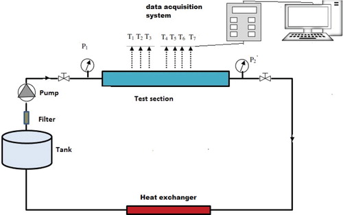
The test section (Figure 2) is a stainless steel duct, its length is 1.2 m. Its cross-section is a rectangle (40 × 25 mm²). Each wall, 10 mm thick, is heated by a rectangular heating panel to provide uniform heating. To reduce heat dissipation, three layers of thermal insulation have been taken into consideration. The first layer is asbestos with a thickness of 5 mm (k_asbestos= 0.15 W/(mK)) which is directly positioned on the thermal heater; the second layer is fiberglass with a thickness of 30 mm (with k_fiberglass= 0.04 W/(mK)) which is applied around the duct; and finally, the third layer is nylon tape (2 mm thick and 50 mm wide with thermal conductivity of 0.25 W/(mK)) to hold all the other layers together. These layers of insulation ensure those heat losses are kept below 5%.

Figure 2. Thermocouple locations in the channel (The dimension is mm).

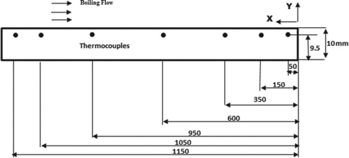
The total power of the input heating panels is 3000 W. A power supply has been used to control the input heating panel. Power supply accuracy is about 1%. The inner wall temperatures are measured with seven K-type thermocouples, located along the duct at axial distances of 50, 150, 350, 600, 950, 1050, and 1150 mm from the duct inlet. They are placed inside the holes and drilled into the duct, 0.5 mm from the upper surface.

Table 1 shows the uncertainty input variables. Applying the proposed method in (Kline & McClintock, 1953), it is estimated that the general uncertainty for measuring the convective heat transfer coefficient is within the range of 1.6% ± 0.8%.

Table 1. Uncertainty in the measured input variables.

Variable $(\chi )$	Uncertainty
Temperature	±0.1°C
Thermal conductivity	±2%
Specific Heat capacity	±2%
Density	±0.5%
Overall uncertainty in the Convective heat transfer coefficient $\frac{\mathrm{\partial }h}{h}=({\sum }_i(\frac{\mathrm{\partial }h}{\mathrm{\partial }{\chi }_i}\frac{\mathrm{\partial }{\chi }_i}{h}{)}^2{)}^{1/2}$

Problem description

The Tikonov technique has been employed to predict heat fluxes into the fluid in a rectangular channel. The channel is made of AISI 313. The heat flux is equal to the heater power. Temporal and spatial variations of heat flux and surface temperature at y = E (Figure 3(a)) are unknown. Around the channel is insulated to minimize heat dissipation. The heat losses which estimated to be lower than 7%. It has been assumed that the loss of heat is negligible with the governing equation of the plate (Farahani & Kowsary, 2014), written as: (1) $\begin{array}{rl}& T_{xx}+T_{yy}={\alpha }^{-1}{T}_t\\ & T_x|{}_{x=0,L}=0\\ & T_y|{}_{y=0}=-q_w{k}^{-1}\\ & T_y|{}_{y=E}=-q(x,t)k^{-1}\\ & T(x,y,0)=T_i\end{array}$(1) where $T_i$, L, E, and $q_w$are the initial temperature, length, and thickness of the plate, and heater power, respectively. $q(x,t)$ is unknown; thus, instead of the heat flux, the measured temperatures by the thermocouples are available from the experimental test. The temperature of the channel wall is affected by the changes in the Nusselt number. We used this matter and solved the problem to predict indirectly the convective heat transfer coefficient (h). First, the $q(x,t)$ is estimated and then $h$ is estimated by using Newton’s cooling law and estimated $q(x,t)$. Thus, we modeled the heat conduction equation (Equation (1)) in the channel wall and the convection term has appeared in the boundary condition. This term is unknown. The measured data contains information about $h$, which can be achieved by the decoding method. The Tikhonov method as the inverse technique, has been used to retrieve this information. The temperatures are measured inside the plate using the thermocouples. These measurements are as input in the inverse technique. The most important point of this technique is that no information is required from the fluid flow field.

Figure 3. (a) Boundary conditions in problem and (b) Inverse algorithm.

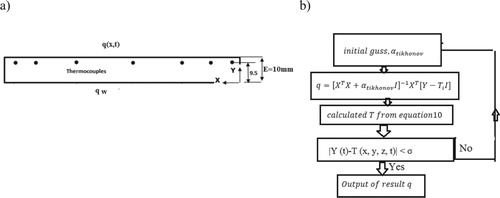
In order the heat conduction equation (Equation (1)) solving, the Finite-Element Method has been used in ANSYS software. In the direct thermal problems, all boundary conditions and material properties (Table 2) are known. The specific heat capacity of the plate was measured by a differential scanning calorimeter (Mettler Toledo DSC-1) in the range of 10–100°C. The bulk density of the plate was measured by dividing its mass per its volume. The thermal conductivity of the plate was measured with a heat flow meter device (Taurus TCA 200). Table 3 shows the location of thermocouples within the plate. The inverse method, the Tikhonov method, estimates the $q(x,t)$, using the temperatures that are recorded from specified positions in the plate. The details of the Tikhonov algorithm have been presented in (Tikhonov, 1975), thus, they will not be brought here. The inverse method employs a parameter, called the sensitivity coefficient, in fact indicating the temperature sensitivity of the unknown parameter. The sensitivity coefficient (Beck, Blackwell, & Clair, 1985) is calculated as: (2) $X(x_m,y_m,t)=\frac{\mathrm{\partial }T(x_m,y_m,t)}{\mathrm{\partial }q}m=1,2,\cdots ,Ns$(2) where x_m and y_m are the sensor location within the channel wall, and P is the number of sensors. It must be noticed that the number of unknowns should be smaller or equal to the number of thermocouples in IHCP (Beck, Blackwell, & Clair, 1985). No functions have been employed to predict the heat flux components. One of the principles of inverse heat transfer is that we have no knowledge about the unknowns. The flow chart of which is illustrated in Figure 3(b), showing an inverse method. Also, See Beck, Blackwell, and Clair (1985) for more details. The regularization parameter in the Tikhonov method is ${\alpha }_{\text{tikhonov}}$. In this study, ${\alpha }_{\text{tikhonov}}$ is ${10}^{-5}$. In this study utilizes seven thermocouples. At least one thermocouple is required to estimate each heat flux component in IHCP (Farahani & Kowsary, 2014). In order to describe heat flux on the heat exchange surface, this study estimates seven parameters, q₁, q₂, … , and q₇, which vary with time. Error analysis is done to determine the accuracy of the proposed algorithm. As such, this analysis is performed, considering AISI304 as plate material and $q_w=cte$. Moreover, a known heat flux at the heat exchange surface (i.e. $q_{\text{exact}}$) and the initial workpiece temperature of 25°C.

Table 2. Thermal property of work material.

Thermal property	Value
Specific heat,$C_p$ (J/(kg.K))	460
$k$ (W/(m.k))	28.6
Density,$\rho (kg/m^3)$	7760

Table 3. Thermocouple position coordinates.

Thermocouple no.	X (mm)	Y (mm)
T1	50	−0.5
T2	150	−0.5
T3	350	−0.5
T4	600	−0.5
T5	950	−0.5
T6	1050	−0.5
T7	1150	−0.5

Temperatures, obtained as a result of a known imposed $q_{\text{exact}}$, are perturbed by noise with (σ = 0.1°C). These temperatures were used to predict the $q$ on each interval. Root mean square error, bias error, and variance error are calculated in error analysis of the inverse technique. The mean squared error is used to check the accuracy of the estimation. This error (Farahani & Kowsary, 2014) is calculated as (3) $\text{RMS}=\sqrt{\frac{1}{N}\sum _{i=1}^N{({\hat{q}}_{i,\text{noisydata}}-q_i)}^2}$(3) where ${\hat{q}}_{i,\text{noisydata}}$ is the predicted heat flux. Bias error (Farahani & Kowsary, 2014) is because of the regularization method and can be calculated as follows: (4) $D=\sqrt{\frac{1}{N}\sum _{i=1}^N{({\hat{q}}_{i,\text{nonoise}}-q_i)}^2}$(4)

In which ${\hat{q}}_{i,\text{nonoise}}$ is estimated using temperatures with$\sigma =0$. The inverse method’s sensitivity to the measurement errors in the data is called the variance error (Farahani & Kowsary, 2014) and can be calculated as: (5) $V=\text{RM}{\text{S}}^2-D^2$(5) For better comparison, the errors have the same scale; hence the second root of the variance is used here. It is necessary for every experimental test that an experimental design should be carried out. This work is also done in this study. In the inverse problem, it is quite clear that the sensors should be closer to the active surface (i.e. boiling surface), and the accuracy of this approach is higher due to the high sensitivity coefficient. In this experiment, the temperature sensors were located at $y=E-0.5\text{mm}$ due to the precision of the machining equipment. In IHCP (Farahani & Kowsary, 2012, 2014), a small-time step causes an increase in the variance error, and a very large time step increases the bias error. We are looking for a suitable time step that the RMS error is low, and we can reach more details about the unknown parameter over time. The time step is determined according to the RMS. The time step is considered 0.01, 0.05, 0.1 and 0.5 s and using the numerical simulation experiments, the error is calculated and is equal to values 0.8 q_mean, 0.05 q_mean, 0.069 q_mean and 0.072 q_mean, respectively. According to the results, 0.1 s is selected. It should be noted that the smallness of the sensitivity coefficient has a direct effect on the increase of RMS error.

Table 4 presents the error analysis for estimated heat flux on the heat exchange surface. Results show that the proposed method has a low error, estimating heat flux. This error is almost 0.06 q_mean. In the proposed method, firstly, the $q(x,t)$ is predicted, and then, using Newton’s cooling law, $h$ is calculated; therefore, the $h$ is estimated indirectly. The proposed algorithm is simple and easy to use, with its results showing it has good accuracy.

Table 4. Error analysis for the purposed inverse method.

Error	RMS(W/m^2)	Bias(W/m^2)	variance(W/m^2)
Estimated heat flux	0.069 × qmean	2.4e−14 × qmean	0.069 × qmean

Results

The $h(x,t)$ is calculated using the $q(x,t)$, itself estimated by the inverse method $(q(x,t))$ and the calculated local surface temperature $(T_s(x,t))$ as follows as: (6) $h(x,t)=\frac{q(x,t)}{T_s(x,t)-T_f(x,t)}$(6) where $T_f(x,t)$ is the bulk temperature and is calculated, using the energy balance equation: (7) $T_f(x,t)=T_f(x-\mathrm{\Delta }x,t)+\frac{q(x,t)(2H+2W)\mathrm{\Delta }x}{\dot{m}{C}_P}$(7)

In which q and T_s are estimated through solving IHCP, $H$ is channel height, and $W$ channel width. The heat transfer coefficient $(\text{Nusselt number})$ (Frances et al., 2019) is specified as follow as: (8) $\text{Nu}(x,t)=\frac{h(x,t)}{k}\left(2\frac{HW}{H+W}\right)$(8)

This study investigates $h(x,t)$ for flow with and without phase change. Several experiments were tested in this study. Considering the number of thermocouples and time-steps, millions of temperatures were acquired as raw data, which we couldn’t present here. Figure 4 illustrates the measured temperatures at x = 0.05, 0.5 and 1.5 m in the flow without phase change (Re = 770) and in liquid–vapor phase flow $\text{G}=355$ kg/(m².s). An increase in temperature is observed with increasing$x$. Also, temperature increases over time.

Figure 4. The measured temperatures for (a)single-phase (Re = 770) and (b) two-phase flow(G = 355 kg/(m².s)).

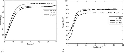
As the flow of fluid enters the channel $(\text{at}x=0)$, the thermal boundary layer forms and develops. The Nusselt number in the channel entrance $(\text{at}x=0)$, is very large. With the growth of the thermal boundary layer along the channel, the Nusselt number reduces until the flow (thermal and hydrodynamic) is fully developed. At this time, the heat transfer coefficient does not change with$x$ and is constant. It can be seen that the flow (Re = 770) reached a steady state after 30 min. Figure 4(b) shows that after 20 min $\mathrm{\partial }T/\mathrm{\partial }t$ is almost constant and is close to zero. However, we have reached a steady state. Slight fluctuations can be seen in this area, which is due to bubble and liquid flows in two-phase flow. During the two-phase flow, the temperature increases along the channel. First, the temperature increases with the time it starts to boil and the bubble is generated inside the stream; in this case, the temperature reaches a constant value. In fact, measurements emphasize this issue the essence of the flow inside the channel strongly affects surface temperature variations.

Single-phase flow

The effect of $Re$ changes on $\text{Nu}(x.t)$ in the single-phase flow has been studied. The obtained results for single-phase flow are validated with Equation (10). Churchill and Ozoe (1973) used experimental results to find a correlation to predict the Nusselt number in a fully developed plug flow in a pipe with $q=cte$. A closed-form expression (Churchill & Ozoe, 1973) for the $\text{N}{\text{u}}_x$, covering both the developing and developed flow in a tube with $q=cte$is:

(9) $\begin{array}{rl}& \frac{\text{N}{\text{u}}_x}{4.364{[1+{(Gz/29.6)}^2]}^{1/6}}\\ & ={[1+{\left(\frac{Gz/19.04}{{[1+{(Pr/0.0207)}^{2/3}]}^{1/2}{[1+{(Gz/29.6)}^2]}^{1/3}}\right)}^{3/2}]}^{1/3}\\ & Gz=\pi /(4x/\mathrm{Re}Pr),\mathrm{Re}=4\dot{m}/\pi \mu D_h,\end{array}$(9) For all Gz, this equation agrees within 5% error in developing flow, and a 3.5% error developed a flow for Pr = 0.7 and Pr = 10. In calculating the Nusselt number for non-circular cross-sections, a hydraulic diameter is utilized. In these cross-sections, the Wall-Stream effect must be considered in calculating the Nusselt number based on the hydraulic diameter $(D_h=(2HW/H+W))$. This correction (Bejan, 2013) is done using the coefficient of $\beta =((\pi D_h^2)/4)/A_{duct}$. Based on the modification of obtained $\text{N}{\text{u}}_x$ extracted from Equation (9), it could be rephrased as (Bejan, 2013): (10) $\text{N}{\text{u}}_x=\text{N}{\text{u}}_x\times \beta$(10)

The importance of β can be seen in Equation (10).

Also, Figure (5) illustrates the estimated time distribution of the heat transfer coefficient at the location of sensors for Re = 1165. $\text{N}{\text{u}}_1,\text{N}{\text{u}}_2,\text{N}{\text{u}}_3,\text{N}{\text{u}}_4,\text{N}{\text{u}}_5,\text{N}{\text{u}}_6\text{and}\text{N}{\text{u}}_7$ is Nusselt number at x = 0.05, 0.15, 0.35, 0.6, 0.95, 1.05 and 1.15 m, respectively. Table 5 gives the difference of estimated $\text{Nu}$ values with the values calculated from Equation (10), showing the highest and lowest difference to be 18% and 0.4%, respectively. The deviation in the Table 5 is $\frac{\text{Estimated}\text{Nu}\text{ - }\text{Extracted}\text{Nu}}{\text{Extracted}\text{Nu}}\ast 100$. A comparison of the estimated single-phase Nu with one predicted (Equation (10)) for laminar flow in rectangular channels is shown in Figure 6(a), wherein time-averaged estimated Nu is compared with the values, obtained from Equation (10). At the present work, and the difference of values calculated from the two correlations is about 7%, and the results are approximately one. Perhaps because the geometry is simple and this affects the flow structure. The $\text{N}{\text{u}}_x$ for Re = 770, 1165 and 1800 is illustrated in Figure 6. Furthermore, the averaged deviation percentage of estimated Nusselt number with the results of Equation (10) for Re = 770, 1165 and 1800 is given in Table 6. The relative deviation is about 2%. Quite obviously, the reason for the deviations is the method for the prediction of the$\text{Nusselt number}$. Table 6 shows where the predicted values fully agree with Equation (10). The mentioned method has good accuracy to estimate the heat transfer coefficient. It shows that the proposed method can successfully estimate the Nusselt number for flow without phase change.

Figure 5. The estimated time history of Nusselt number of single-phase flow at the position of sensors for Re = 1165.

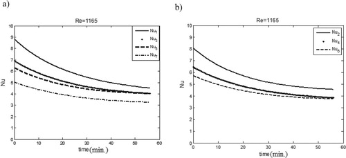
Figure 6. The local Nusselt number along the channel length for (a) Re = 770, (b) Re = 1165 and (c) Re = 1800.

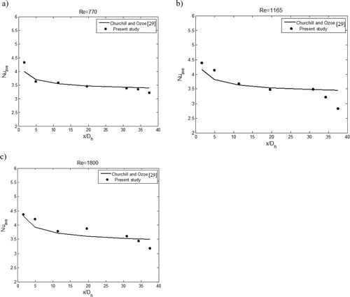
Table 5. Deviation between the extracted Nu from Equation (10) and estimated Nu.

No.	Location (m)	$\text{Extracted Nu}$	$\text{Estimated Nu}$	Deviation (%)
1	0.050	4.450	4.220	−5.4
2	0.150	4.197	3.870	−8.4
3	0.350	3.729	3.680	−1.3
4	0.600	3.523	3.588	1.8
5	0.950	3.537	3.523	−0.4
6	1.050	3.270	3.510	6.8
7	1.150	2.873	3.499	17.8

Table 6. Mean deviation between the estimated Nu and calculated Nu from Equation (10).

	Re = 1165	Re = 1800	Re = 770
Equation (10)	3.60	3.78	3.56
Estimated	3.64	3.73	3.56
Error	0.011	−0.014	−0.001

Boiling flow

Table 7 gives the experimental conditions for boiling flow. The mass flux $(G=\dot{m}/(HW))$ varies between 118.1 and 355 kg/(m2.s), whereas the $q_w$ is from 0 to 19.2 kW/m². Figure 7 shows time variations of the estimated $q(x,t)$ on the heat exchange surface for G = 234 kg/(m² s). Nusselt number for boiling flow is calculated using Equation (6), in which $T_f(x.t)$ will be equal to saturation temperature, $T_{sat}$.

Figure 7. The time history of the local heat flux along the channel length.

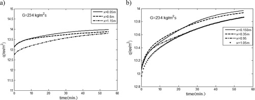
Table 7. Mass flux and heat flux for two-phase flow.

G(kg/(m2.s))	118.1	234	355
qw(kW/m2)	7.9	14	18.9

To compare the Nusselt number of boiling flow inside the tube, it has been applied to the correlation that Kandlikar (1990) has been given. Kandlikar’s correlation is (11) $\begin{array}{rl}\text{Nu}& =\text{N}{\text{u}}_{\text{sp}}[0.6683C{o}^{-0.2}{\left(25\frac{G^2}{{\rho }_L^{2}g{D}_h}\right)}^{0.3}\\ & +1058{\left(\frac{q}{G{h}_{fg}}\right)}^{0.7}]\end{array}$(11) where Nu_sp is the Nusselt number in the single-phase state and is calculated by assuming that all flow inside the channel is liquid and Co is the convection number, defined by Kandlikar (1990): (12) $Co={\left(\frac{1-x_v}{x_v}\right)}^{0.8}{\left(\frac{{\rho }_G}{{\rho }_L}\right)}^{0.5}$(12)

In which $x_v.{\rho }_L.\text{and}{\rho }_G$ are the local vapor quality, the density of liquid and vapor, respectively. Kandlikar’s correlation (Equation (11)) is further refined by expanding the database to 5246 data points from 24 experimental investigations with 10 fluids. This correlation gives a mean deviation of 15.9 percent with water data, and 18.8 percent with all refrigerant data (Kandlikar, 1990). In order to specify the quality of vapor, the energy equilibrium equation for every section between the input and the output is employed. The vapor mass qualities (Kandlikar,1990) is calculated as: (13) $\begin{array}{rl}{X}_v(x,t)& =X_v(x-\mathrm{\Delta }x,t)+\frac{1}{h_{fg}}[2\frac{q(x,t)(H+W)}{\stackrel{.}{m}}\mathrm{\Delta }x\\ & -C_P(T_{sat}-T_f(x,t))\phantom{2\frac{q(x,t)(H+W)}{\stackrel{.}{m}}\mathrm{\Delta }x}]\end{array}$(13) Figure 8(a) shows the time-averaged Nu decreases with increasing $x$ and the experimental results are close to the predictions of Kandlikar. Near the entrance of the channel is the difference between the estimated values and the reference values (Kandlikar, 1990) at about 19% and in the rest of the regions, this difference is insignificant. The reason for this difference between the empirical correlations with the present work can be attributed to how the heat flux is calculated at the $y=E$, in these two empirical correlations, the authors have assumed that$q(x.t)=q_w$. Another reason may be that the curve fitting of the experimental data has errors and the results of the correlation on the test data are not fully matched.

Figure 8. (a) The local convective heat transfer coefficient along the channel length, and (b) time variation of local vapor quality along the channel length.

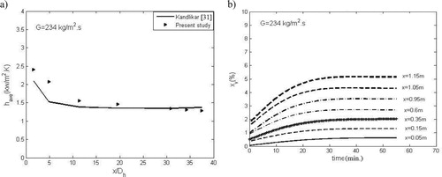
The time distribution of vapor quality along the channel is illustrated in Figure 8(b). The quality of the vapor increases in the flow direction along the channel, thanks to the bubble coalescence mechanism; therefore, the frequency of the bubbles is reduced. This explains why heat transfer is reduced when the quality of steam is increased. It can be determined when the vapor generation along channel length starts, as it is one of the findings of the proposed method. The heat transfer of boiling flow consists of the convective and the nucleate boiling terms. Using the proposed method, the role of each component can be determined.

Figures (9) and (10) demonstrate the variations of $Co\text{number}$ and $Bo\text{number}$ with time. Convection number decreases with time, similar to the trend of changes in Convection number along the channel, which descends as well. The maximum amount of Co corresponds to the 50 mm distance from the channel entrance. The boiling number at the measurement points increases with time. Temporal and spatial Variations of Boiling number is similar to the variations of the predicted heat flux. The nucleate boiling heat transfer is dominant when the $Co$ number is too large. In the nucleate boiling region, the $\text{Nu }$ is a weak function of the convection number because the mechanism of convection has little effect in this area and is not the dominant mechanism. In the area where the convective boiling mechanism is dominant, the amount of convection number is small. The contribution of the convective boiling decreases when the Boiling number is increased. Figure 11 illustrates the variations in the time-averaged of Nusselt number for G = 118.1, 234, and 355 kg/(m².s) with the quality of vapor. As the figure shows the Nusselt number reduces with an enhancement in$X_v$. 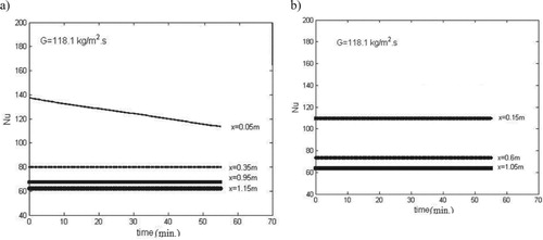The $X_v$ is low when the nucleate boiling is dominant. This mechanism and convective heat transfer help to enhance the heat transfer. The time distribution of local Nusselt number for G = 118.1 kg/(m².s) is presented in Figure 12. At x = 50 mm, the number varies with time but does not change much in other measurement points.

Figure 9. The variations of Boiling number (Bo) with time along the channel.

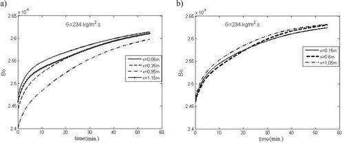
Figure 10. The variations of convection number (Co) with time along the channel.

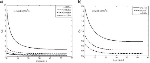
Figure 11. Time-averaged heat transfer coefficient with the vapor quality.

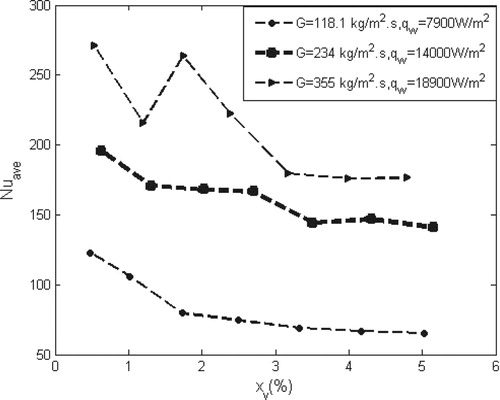
Figure 12. The time variation of local Nusselt number for G = 118.1 kg/(m².s).

Conclusions

This research conducted a laboratory investigation of water flow with and without phase change in a channel. The temperatures within the wall were experimentally measured, providing the input data for the inverse method to predict the $q(x,t)$. The transient analysis was performed. First, the experiment was designed and error analysis carried out to determine the accuracy of the proposed method. RMS error for estimation heat flux was around 0.06 q_mean. Using Newton’s cooling law and estimated values of heat flux, temporal and spatial distribution of Nusselt number was predicted. The time-averaged local Nusselt number estimated for flow with and without phase change was close to those, predicted by the correlations of Churchill and Ozoe (1973) and Kandlikar (1990), respectively. It was seen in boiling flow that local quality of vapor and the boiling number increased and local convection number decreased with time. Also, along the length of channel time-averaged Nusselt number decreased with the quality of vapor. The temporal and spatial changes of the Convective number and the Boiling number can be determined using the proposed method. The maximum amount of Co corresponds to the 50 mm distance from the channel entrance. This helps better understanding the boiling phenomenon. For future research employing artificial intelligence methods, in particular, machine learning techniques (e.g. Farzaneh-Gord et al., 2019; Ghalandari, et al., 2019a, 2019b; Menad et al., 2019; Mosavi, Shamshirband, Salwana, Chau, & Tah, 2019; Mou, He, Zhao, & Chau, 2017) is encouraged considering higher accuracy and lower computational costs.

Disclosure statement

No potential conflict of interest was reported by the authors.

References

- Ahmadi, M. H., Ghahremannezhad, A., Chau, K., Seifaddini, P., Ramezannezhad, M., & Ghasempour, R. (2019). Development of simple-to-use predictive models to determine thermal properties of Fe2O3/water-ethylene glycol nanofluid. Computation, 7(1), 18. doi: 10.3390/computation7010018
- Aiba, S., & Yamazaki, Y. (1976). An experimental investigation of heat transfer around a tube in a bank. Journal of Heat Transfer, 98(3), 503–508. doi:10.1007/BF00997314 doi: 10.1115/1.3450583
- Babu, K. T., & Kumar, S. P. (2010). Mathematical modeling of surface heat flux during quenching. Metallurgical and Materials Transactions B: Process Metallurgy and Materials Processing Science, 41(1), 214–224. doi: 10.1007/s11663-009-9319-y
- Beck, J. V., Blackwell, B., & Clair, C. R. S. (1985). Inverse heat conduction: Ill-posed problems. New York, NY: Wiley Interscience.
- Bejan, A. (2013). Convection heat transfer (4th ed.). Cleveland, OH, USA: John Wiley & Sons, Inc.
- Bohdal, T. (2001). Development of bubbly boiling in channel flow. Experimental Heat Transfer, 14(3), 199–215. doi: 10.1080/08916150121317
- Boudouh, M., Gualous, H. L., & Labachelerie, M. D. (2010). Local convective boiling heat transfer and pressure drop of nano fluid in narrow rectangular channels. Applied Thermal Engineering, 30, 2619–2631. doi: 10.1016/j.applthermaleng.2010.06.027
- Bozzoli, F., Cattani, L., Rainieri, S., Bazán, F. S. V., & Borges, L. S. (2014). Estimation of the local heat-transfer coefficient in the laminar flow regime in coiled tubes by the Tikhonov regularization method. International Journal of Heat and Mass Transfer, 72, 352–361. doi: 10.1016/j.ijheatmasstransfer.2014.01.019
- Buongiorno, J. (2006). Convective transport in nanofluids. Journal of Heat Transfer, 128(3), 240–250. doi: 10.1115/1.2150834
- Cattani, L., Bozzoli, F., & Rainieri, S. (2017). Experimental study of the transitional flow regime in coiled tubes by the estimation of local convective heat transfer coefficient. International Journal of Heat and Mass Transfer, 112, 825–836. doi: 10.1016/j.ijheatmasstransfer.2017.05.003
- Chen, J., & Li, W. (2018). Local flow boiling heat transfer characteristics in three-dimensional enhanced tubes. International Journal of Heat and Mass Transfer, 121, 1021–1032. doi:10.1016/ j.ijheatmasstransfer. 2018.01.065 doi: 10.1016/j.ijheatmasstransfer.2018.01.065
- Churchill, S. W., & Ozoe, H. (1973). Correlations for force convection with uniform heating in flow over a plate and in developing a fully developed flow in a tube. Journal of Heat Transfer, 95, 78–84. doi: 10.1115/1.3450009
- Farahani, S. D., & Kowsary, F. (2012). Estimation local convective boiling heat transfer coefficient in mini channel. International Communications in Heat and Mass Transfer, 39, 304–310. doi: 10.1016/j.icheatmasstransfer.2011.11.007
- Farahani, S. D., & Kowsary, F. (2014). Direct estimation local convective boiling heat transfer coefficient in mini channel by using conjugated gradient method with adjoint equation. International Communication Heat and Mass Transfer, 3, 4–10. doi: 10.1016/j.icheatmasstransfer.2014.03.004
- Farzaneh-Gord, M., Faramarzi, M., Ahmadi, M. H., Sadi, M., Shamshirband, S., Mosavi, A., & Chau, K. W. (2019). Numerical simulation of pressure pulsation effects of a snubber in a CNG station for increasing measurement accuracy. Engineering Applications of Computational Fluid Mechanics, 13(1), 642–663. doi: 10.1080/19942060.2019.1624197
- Frances Viereckl, F., Christoph, E. S., Wolfgang, S., & Hurtado, A. L. (2019). Experimental and theoretical investigation of the boiling heat transfer in a low-pressure natural circulation system. Experimental and Computational Multiphase Flow, 1(4), 286–299. doi: 10.1007/s42757-019-0023-0
- Ghahremannezhad, A., & Vafai, K. (July 2018). Thermal and hydraulic performance enhancement of microchannel heat sinks utilizing porous substrates. International Journal of Heat and Mass Transfer, 122, 1313–1326. doi:10.1016/j.ijheatmasstransfer.2018.02.02 doi: 10.1016/j.ijheatmasstransfer.2018.02.024
- Ghalandari, M., Bornassi, S., Shamshirband, S., Mosavi, A., & Chau, K. W. (2019a). Investigation of submerged structures’ flexibility on sloshing frequency using a boundary element method and finite element analysis. Engineering Applications of Computational Fluid Mechanics, 13(1), 519–528. doi: 10.1080/19942060.2019.1619197
- Ghalandari, M., Ziamolki, A., Mosavi, A., Shamshirband, S., Chau, K. W., & Bornassi, S. (2019b). Aeromechanical optimization of first row compressor test stand blades using a hybrid machine learning model of genetic algorithm, artificial neural networks and design of experiments. Engineering Applications of Computational Fluid Mechanics, 13(1), 892–904. doi: 10.1080/19942060.2019.1649196
- Giedt, W. H. (1949). Investigation of variation of point unit heat-transfer coefficient around a cylinder normal to an air stream. ASME Transaction, 71, 375–381.
- Huang, H., Lamaison, N., & Thome, J. R. (2017). Transient data processing of flow boiling local heat transfer in a multi-microchannel evaporator under a heat flux disturbance. Journal of Electronic Packaging, 139, 11005–11010. doi: 10.1115/1.4035386
- Kandlikar, S. G. (1990). A general correlation for saturated two-phase flow boiling heat transfer inside horizontal and vertical tubes. ASME Journal of Heat Transfer, 112, 219–228. doi: 10.1115/1.2910348
- Kim, S., & Mudawar, I. (2013). Universal approach to predicting saturated flow boiling heat transfer in mini/micro-channels – Part II. Two-phase heat transfer coefficient. International Journal of Heat and Mass Transfer, 64, 1239–1256. doi: 10.1016/j.ijheatmasstransfer.2013.04.014
- Kline, S. J., & McClintock, F. A. (1953). Describing experimental uncertainties in single sample experiment. Mechanical Engineering, 75(1), 3–8.
- Kuznetsov, V. V. (2019). Fundamental issues related to flow boiling and two-phase flow patterns in microchannels – Experimental challenges and opportunities. Heat Transfer Engineering, 40, doi: 10.1080/01457632.2018.1442291
- Lee, S., Choi, S. U. S., Li, S., & Eastman, J. A. (1999). Measuring thermal conductivity of fluids containing oxide nanoparticles. Journal of Heat Transfer, 121(2), 280–289. doi: 10.1115/1.2825978
- Menad, N. A., Noureddine, Z., Hemmati-Sarapardeh, A., Shamshirband, S., Mosavi, A., & Chau, K. W. (2019). Modeling temperature dependency of oil-water relative permeability in thermal enhanced oil recovery processes using group method of data handling and gene expression programming. Engineering Applications of Computational Fluid Mechanics, 13(1), 724–743. doi: 10.1080/19942060.2019.1639549
- Mosavi, A., Shamshirband, S., Salwana, E., Chau, K. W., & Tah, J. H. (2019). Prediction of multi-inputs bubble column reactor using a novel hybrid model of computational fluid dynamics and machine learning. Engineering Applications of Computational Fluid Mechanics, 13(1), 482–492. doi: 10.1080/19942060.2019.1613448
- Mou, B., He, B. J., Zhao, D. X., & Chau, K. W. (2017). Numerical simulation of the effects of building dimensional variation on wind pressure distribution. Engineering Applications of Computational Fluid Mechanics, 11(1), 293–309. doi: 10.1080/19942060.2017.1281845
- Ozisik, M. N., & Orlande, H. R. B. (2000). Inverse heat transfer-foundation and applications. San Francisco, California: Taylor & Francis, USA state.
- Rao, S. (1996). Engineering optimization: Theory and practice (3rd ed.). San Francisco, California: Wiley.
- Rouizi, Y., Al Hadad, W., Maillet, D., & Jannot, Y. (2015). Experimental assessment of the fluid bulk temperature profile in a mini channel through inversion of external surface temperature measurements. International Journal of Heat and Mass Transfer, 83, 522–535. doi: 10.1016/j.ijheatmasstransfer.2014.12.031
- Saisorn, S., Wongpromma, P., & Wongwises, S. (2018). The difference in flow pattern, heat transfer and pressure drop characteristics of mini-channel flow boiling in horizontal and vertical orientations. International Journal of Multiphase Flow, 101, 97–112. doi:10.1021/i260019a023 doi: 10.1016/j.ijmultiphaseflow.2018.01.005
- Taler, J. (2007). Determination of local heat transfer coefficient from the solution of the inverse heat conduction problem. Forschung im Ingenieurwesen, 71(2), 69–78. doi: 10.1007/s10010-006-0044-2
- Thome, J. R., & El Hajal, J. (2003). Two – phase flow pattern map for evaporation in horizontal tubes: Latest version. Heat Transfer Engineering, 24(6), 3–10. doi: 10.1080/714044410
- Tibiriça, C. B., & Ribatski, G. (2011). Two-phase frictional pressure drop and flow boiling heat transfer for R245fa in a 2.32 mm tube. Heat Transfer Engineering, 32(13), 1139–1149. doi: 10.1080/01457632.2011.562725
- Tikhonov, A. N. (1975). Inverse problems in heat conduction. Journal of Engineering Physics, 29, 816–820. doi: 10.1007/BF00860616
- Wadekar, V. V. (2012). Hydraulic characteristics of flow boiling of hyrdocarbon fluids: Two phase pressure drop. Heat Transfer Engineering, 33(9), 786–791. doi: 10.1080/01457632.2012.646865