Large eddy simulations of wind loads on an external floating-roof tank

Abstract

Wind load of an external floating-roof tank is analyzed using large eddy simulation (LES). First, the governing equations and a LES solution procedure employing FLUENT software are presented. Subsequently, using two benchmark tank models, the accuracy of LES is examined and the advantages of LES over wind Reynolds-averaged Navier-Stokes (RANS) method in computing the unsteady wind loads and vortex structures around a tank are validated. Finally, using LES, the turbulent flows and wind loads around an external floating-roof tank at varying Reynolds numbers and liquid levels are analyzed. The DSM SGS model was found to have better accuracy when LES is applied to the tank flow. For an external floating-roof tank, the Reynolds number has little influence on the wind load at Re > 10⁶, while the liquid level affects significantly both the wind loads on the tank and the vortex structures in the flow, and the wind pressure on the internal wall distributes more evenly than that on the external wall, due to the recirculation of the flow in the cavity above the roof. In all cases, the pressure on the external floating-roof tank oscillates apparently with time, which indicates the necessity of applying LES to the wind load analysis of tanks.

KEYWORDS:

• Floating-roof tank
• wind load
• liquid level
• large eddy simulation
• numerical simulation

1. Introduction

For the purpose of energy security, a great number of state oil strategic reserves have been built worldwide. In aboveground oil storage reserves, external floating-roof tanks with capacities above 10⁵m³ are usually used to store the crude oil. As the name implies, an external floating-roof tank is mainly constructed by a metal cylindrical shell and a steel floating roof. Compared with the fixed roof tanks used widely in stations of oil fields and oil pipelines, the cylindrical shell of external floating-roof tanks has much larger radius to thickness ratio, which is usually in an order of 1000∼2000. As a typical thin-walled structure, the external floating-roof tanks, especially for those located in the coastal area, usually experience the buckling problem under wind load. In strong winds such as typhoon and tornado, buckling-induced deflection of the cylindrical shell might incline significantly the floating roof or even destroy the whole tank (Godoy, 2007; Portela, Virella, & Godoy, 2006). To reveal the buckling characteristics of an external floating-roof oil storage tank, investigating first the features of wind load, as well as the unsteady flow around it, is of vital importance.

In the past decades, many experimental or numerical studies have been conducted on the wind loads of tanks or shells of various shapes. In experimental investigations, the boundary layer wind tunnels are usually employed to test the pressure distribution and the flow field around the small-scale models. Acheinbach (1968, 1972) investigated the effects of the Reynolds number (Re), turbulence intensity and surface roughness on the wind load of a two-dimensional (2D) cylinder model in the wind tunnel. The experiments showed that there is a critical Reynolds number of about 10⁵, above which the pressure distribution on the cylinder surface is almost independent of Re. Later, this finding was confirmed by Mulhearn, Banks, Finnigan, and Annis (1976) and Macdonald, Kwok, and Holmes (1988). Greiner and Derler (1995) carried out experiments on cylindrical shells with H/D = 10 and 0.5. They observed that, compared with the short shell, the pressure on the external wall of the long shell varies more significantly in the axial direction. Probert, Hasoon, and Lee (1973) and Holroyd (1983) employed the visualization technique to analyze flow features around the tanks with H/D = 0.345 and 0.87 at Re = 3.5×10⁶∼2.7×10⁷. It was found that the angle of the wake behind the tank is changed with the height to diameter ratio and the Reynolds number. Holroyd (1983) also observed that the flow outside the tank and below its rim is hardly affected by the height of the roof. Lin and Zhao (2014) studied the effect of the roof configuration on the wind load of a tank with H/D = 0.275. They indicated that the pressure distribution on the tank body is not affected much by the roof configuration. Uematsu, Koo, and Yasunaga (2014) conducted a wind tunnel experiment for an open-topped tank model with H/D = 0.25, 0.5 and 1.0 at Re = 1.6×10⁵. They reported that the time-averaged pressure coefficient on the internal wall is fluctuating between −0.5 and −0.9.

With rapid developments of computer and computational fluid dynamics (CFD), numerical simulation is playing an increasingly important role in various engineering applications such as the aircraft design (Hannat, Weiss, Garnier, & Morency, 2014), building design (Mou, He, Zhao, & Chau, 2017), power engineering (Akbarian et al., 2018), clean energy (Ardabili et al., 2018), nanotechnology (Ghalandari, Koohshahi, Mohamadian, Shamshirband, & Chau, 2019; Ramezanizadeh, Nazari, Ahmadi, & Chau, 2019), etc. Numerical studies on the wind loads of various tanks were also conducted. Pasley and Clark (2000) employed the Reynolds-averaged Navier-Stokes (RANS) and k-ε turbulence model to simulate the flow structure around an external floating-roof oil storage tank with H/D = 0.5 at Re = 1.3×10⁵∼3.4×10⁷. It was found that the flow structures around an empty tank and a full tank are very distinct. For an empty tank, the flow circulates in the cavity on the top of the tank, while for a full tank the flow re-attaches to the tank roof. Using similar numerical method, Falcinelli, Elaskar, and Godoy (2011) computed the pressure coefficients on the external wall of a conical roof tank with H/D = 0.4 at Re = 3.2×10⁶, 4.27×10⁶ and 6.4×10⁶. In their work, the unstructured grids in the leeside of the tank are not fine enough to capture the high-pressure gradient near the tank wall, and the computed wind pressure is only qualitatively similar to those measured from experiments (Macdonald et al.,1988).

In previous experimental studies, effects of height to radius ratio, roof configuration and Reynolds number on the wind loads of the flat-roof and open-topped tanks are investigated extensively, but less work has been done on the external floating-roof tanks. In the numerical study of Pasley and Clark (2000), the flow field around an external floating-roof tank was simulated. However, since the RANS equations and k-ε turbulence model were employed, only the time-averaged pressure and vortex structures were obtained while the transient flow features were not captured. Recently, a high accuracy algorithm called large eddy simulation (LES) is developed rapidly and applied in various engineering problems (Montazeri & Blocken, 2013; Murakami & Mochida, 1995). Different from the RANS method, which only computes the time-averaged flow parameters, the LES method is capable of capturing the unsteady evolution process of the wind loads and large-scale vortex structures. If LES is employed to analyze the turbulent flow and wind pressure of oil tanks, more accurate and reliable numerical results could be obtained and more unsteady flow features could be revealed. To the best of our knowledge, however, little work has been done on this subject.

The purpose of the present paper is twofold. One is to extend the LES method to the wind flow around a tank, and the other is to study the effects of the Reynolds number and the liquid level on the wind load and vortex structures of an external floating-roof tank. Using the LES method, unsteady flow features of an external floating-roof tank such as the pressure oscillation on the wall and the transient vortex structures in the flow, which have not been captured in previous RANS computations, are revealed. The paper is organized as follows. First, the governing equations and subgrid-scale (SGS) models for the LES method are introduced in Section 2. Section 3 discusses the numerical method. In Section 4, the effects of the SGS model and grid density on the wind load are analyzed employing a benchmark tank model having experimental results, and the numerical results from RANS and LES are compared. Section 5 investigates the wind loads and flow fields of an external floating-roof tank at different Reynolds numbers and liquid levels. Finally, Section 6 is dedicated to the concluding remarks.

2. Governing equations

Considering the Mach number of the natural wind is below 0.3 while the Reynolds number with respect to the tank diameter is usually high, the wind flow around an external floating-roof tank is assumed to be three-dimensional, incompressible and turbulent. Considering the air density is very low, the effect of the gravity is ignored. As is well-known, turbulent flows are characterized by eddies with a wide range of length and time scales. The large-scale eddies are typically comparable in size to the characteristic length of the mean flow, while the small-scale eddies are responsible for the dissipation of the turbulence kinetic energy. In the LES method, the large-scale eddies are resolved directly while the small-scale eddies are modeled, so that the dominant vortex structures in the turbulence flow can be computed with limited computational expense. Based on these assumptions, the governing equations of LES can be obtained as follows by filtering the incompressible Navier-Stokes equations (Pope, 2000) (1) $\begin{array}{rl}\frac{\mathrm{\partial }{\overline{u}}_i}{\mathrm{\partial }{x}_i}& =0\end{array}$(1) (2) $\begin{array}{rl}\frac{\mathrm{\partial }{\overline{u}}_i}{\mathrm{\partial }t}\text{ + }\frac{\mathrm{\partial }{\overline{u}}_i{\overline{u}}_j}{\mathrm{\partial }{x}_j}& =-\frac{1}{\rho }\frac{\mathrm{\partial }\overline{p}}{\mathrm{\partial }{x}_i}+\nu \frac{{\mathrm{\partial }}^2{\overline{u}}_i}{\mathrm{\partial }{x}_j\mathrm{\partial }{x}_j}\text{ + }\frac{\mathrm{\partial }{\tau }_{ij}}{\mathrm{\partial }{x}_j}\end{array}$(2) where ‘¯’ indicates the filtered variables, u_i is the velocity component, x_i is the coordinate component, t is the time, ρ is the air density, p is the pressure, ν is the kinematic viscosity of air and ${\tau }_{ij}$ is the subgrid-scale (SGS) stress tensor, which can be expressed as (3) $\begin{array}{r}{\tau }_{ij}={\overline{u}}_i{\overline{u}}_j-\overline{u_i{u}_j}\end{array}$(3) Because the term $\overline{u_i{u}_j}$ in Equation (3) is unknown and cannot be expressed explicitly by the filtered variables ${\overline{u}}_i$ and $\overline{p}$, Equations (1) and (2) are not closed. To solve this problem, the Boussinesq hypothesis (Hinze, 1975) is employed and the SGS stress is expressed as (4) $\begin{array}{r}{\tau }_{ij}=2{\nu }_{SGS}{\overline{S}}_{ij}-\frac{1}{3}{\tau }_{kk}{\delta }_{ij}\end{array}$(4) where ${\tau }_{kk}$ is the isotropic part of the SGS stress, ${\delta }_{ij}$ is the Kronecker delta, ${\nu }_{SGS}$ is the SGS eddy viscosity and ${\overline{S}}_{ij}$ is the rate-of-strain tensor for the resolved scale, which can be written as (5) $\begin{array}{r}{\overline{S}}_{ij}\text{ = }\frac{1}{\text{2}}\left(\frac{\mathrm{\partial }{\overline{u}}_i}{\mathrm{\partial }{x}_j}+\frac{\mathrm{\partial }{\overline{u}}_j}{\mathrm{\partial }{x}_i}\right)\end{array}$(5) Finally, the effect of the SGS eddy viscosity ${\nu }_{SGS}$ in Equation (4) on the large scales is modeled to close the governing equations. Table 1 presents four SGS models used widely in LES, including the Smargorinsky-Lilly Model (SM), Dynamic Smargorinsky-Lilly Model (DSM), Wall-Adapting Local Eddy-Viscosity Model (WALE) and Algebraic Wall-Modeled LES Model (WMLES). In Table 1, $L_s$ is the mixing length for subgrid scales, $\kappa$ is the von Karman constant, $d$ is the distance to the closest wall, $C_s$ is the Smagorinsky parameter, $\mathrm{\Delta }$ is the local grid scale, ‘^’ indicates the second filtering operation, subscript f is the first filter, subscript g is the second filter, ${\mathrm{\Delta }}_1$ is the first grid filter width, ${\mathrm{\Delta }}_2$ is the second grid filter width, $L_{ij}$ can be computed from the resolved large eddy field, $C_D$ is the dynamic Smagorinsky parameter, $C_w$ is the WALE model coefficient, $d_w$ is the wall distance, $y^{+}$ is the dimensionless wall distance, $h_{max}$ is the maximum edge length for rectilinear hexahedral cell, and $h_{wn}$ is the wall-normal grid spacing. More details about these SGS models refer to Smagorinsky (1963), Erlebacher (1990), Germano, Piomelli, Moin, and Cabot (1991), Lilly (1992), Nicoud and Ducros (1999) and Shur, Spalart, Strelets, and Travin (2008).

Table 1. SGS models used widely in LES.

SGS model	Equations
SM	${\nu }_{SGS}\text{ = }\rho {L_s}^2\sqrt{2{\overline{S}}_{ij}{\overline{S}}_{ij}}$; $L_s=min\left(\kappa d,C_s\mathrm{\Delta }\right)$
DSM	$({\nu }_{SGS}{)}_f=\left(C_D{{\mathrm{\Delta }}_1}^2\sqrt{2{\overline{S}}_{ij}{\overline{S}}_{ij}}\right)$; $({\nu }_{SGS}{)}_g=\left(C_D{{\mathrm{\Delta }}_2}^2\sqrt{2{\hat{S}}_{ij}{\hat{S}}_{ij}}\right)$; $L_{ij}=(\tau {}_{ij}{)}_{fg}-[{\left({\tau }_{ij}\right)}_f{]}_g$; $L_{ij}+\frac{1}{3}{L}_{kk}{\delta }_{ij}=C_D{M}_{ij}$; $M_{ij}=2\left[{{\mathrm{\Delta }}_2}^2\sqrt{2{\hat{S}}_{ij}{\hat{S}}_{ij}}{\hat{S}}_{ij}-{{\mathrm{\Delta }}_1}^2\stackrel{ˆ}{\sqrt{2{\overline{S}}_{ij}{\overline{S}}_{ij}}{\overline{S}}_{ij}}\right]$; $C_D=\frac{⟨M_{ij}{L}_{ij}⟩}{⟨M_{ij}{M}_{ij}⟩}$
WALE	${\nu }_{SGS}=\rho {L_s}^2\frac{{\left({S_{ij}}^d{S_{ij}}^d\right)}^{3/2}}{{\left({\overline{S}}_{ij}{\overline{S}}_{ij}\right)}^{5/2}+{\left({S_{ij}}^d{S_{ij}}^d\right)}^{5/4}}$; $L_s=min\left(kd,C_w{V}^{1/3}\right)$ ; ${S_{ij}}^d=\frac{1}{2}\left({{\overline{g}}_{ij}}^2+{{\overline{g}}_{ji}}^2\right)-\frac{1}{3}{\delta }_{ij}{{\overline{g}}_{kk}}^2$; ${\overline{g}}_{ij}=\frac{\mathrm{\partial }{\overline{u}}_i}{\mathrm{\partial }{x}_j}$
WMLES	${\nu }_{SGS}=min\left[{\left(\kappa d_w\right)}^2,{\left(C_{S_{mag}}\mathrm{\Delta }\right)}^2\right]\sqrt{2{\overline{S}}_{ij}{\overline{S}}_{ij}}\left\{1-\exp \left[-{\left(\frac{y^{+}}{25}\right)}^3\right]\right\}$; $\mathrm{\Delta }=min\left[max\left(C_w{d}_w,C_w{h}_{max},h_{wn}\right),h_{max}\right]$

3. Numerical method

The commercial CFD code FLUENT is employed to solve the governing equations Equations (1) and (2). In FLUENT, the LES solver with the SM, DSM, WALE and WMLES SGS models is available for turbulent flow simulation. To increase the reliability and accuracy, a high-order finite volume scheme and the high-quality structured mesh are used in the present computation. The pressure-implicit with splitting of operators (PISO) scheme is applied for pressure-velocity coupling, the least squares cell-based scheme is employed for gradient discretization, the finite-volume discretization with bounded central differencing scheme is utilized for the filtered momentum equation, the standard scheme is used for pressure interpolation, and the temporal discretization is performed using the bounded second-order implicit scheme. The residuals of x, y, z velocity components and continuity are taken as the convergence monitors. The convergence criteria for them are all set as 10⁻⁵. The dimensionless time step is set as $\mathrm{\Delta }{t}^{\ast }=\mathrm{\Delta }t{u}_{\mathrm{\infty }}/D\approx 0.1$, the maximum iterations in each time step is 200 and the stable solutions are obtained near $t=50\mathrm{\Delta }{t}^{\ast }$. Because the flows around the tanks are turbulent and unsteady in the Reynolds number range considered in this paper, the stable solutions do not mean the steady solutions, but correspond to the results when the oscillating amplitude of each convergence monitor is not changed much with the computing time. Moreover, the data for time statistics are sampled after the stable oscillation of the flow field is achieved.

4. Validation

Before studying the wind load on the external floating-roof tanks, two benchmark tank models with experimental results proposed by Macdonald et al. (1988) are computed first for the purpose of validation. In the experiments of Macdonald et al. (1988), the wind pressures on a flat roof tank and an open-topped tank were tested in the wind tunnel. For the flat roof tank model (M1), the height to diameter ratio is H/D = 1, wall thickness is b = 0.025D, and the Reynolds number with respect to the tank diameter, free-stream velocity and kinematic viscosity of air is Re = 2.9×10⁵. For the open-topped tank model (M2), the height to diameter ratio is H/D = 0.5, wall thickness is b = 0.025D and Reynolds number is Re = 2.5×10⁵.

Figure 1 displays the computational model for two benchmark models. As shown in the figure, the inlet is placed at 5D upstream of the tank and a uniform free-stream velocity is imposed on it. The two side boundaries are located 2.5D from the tank center, where the symmetry boundary conditions are applied. The outlet is 10D downstream and the outflow boundary condition is utilized. The tank is placed on the bottom wall, and the no-slip boundary condition is imposed on the bottom wall and tank surface. The top boundary of the solution domain is 4H high from the bottom wall and the slip boundary condition is applied. The turbulence intensity on the inlet is set at 1.3%, which is exactly the same as that in Macdonald et al. (1988). In all simulations, the turbulence of 1.3% is applied directly on the inlet of the flow domain, not as a combination of turbulent kinetic energy and dissipation.

Figure 1. A computational model for the turbulent flow around the flat roof and open-topped tank models (Macdonald et al., 1988).

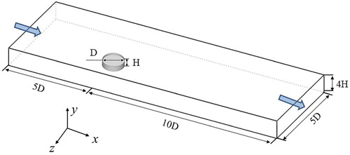
Figure 2 illustrates the computational meshes generated by ICEM CFD for the tank models M1 and M2 (M1-2, M2-2). As seen in the figure, the structured hexahedral grids are utilized to discretize the solution domain. On the surfaces of the tank and bottom wall, the body-fitted grids are used to capture the boundary layer and near-wall vortices. To meet the requirements of LES on computational mesh, the maximum y⁺ of the first layer mesh attached to the surfaces of the tank and bottom wall is set as $y^{+}\approx 1$ and the maximum stretching ratios of the hexahedral grid elements is set as $r=1.2$, which is less than the required stretching ratio $r\le 1.3$ for LES suggested by Tominaga et al. (2008). To test the effect of grid density on the computed wind load on the tank, another two meshes are generated for each tank model (M1-1, M1-3 for the flat roof tank and M2-1, M2-3 for the open-topped roof tank). One (M1-1 and M2-1) is coarser while the other (M1-3 and M2-3) is finer than the mesh presented in Figure 2. To examine the effect of solution domain size, another two meshes, namely M1-4 and M2-4, are generated for the flat roof tank and the open-topped roof tank models, respectively. For M1-4 an M2-4, the inlet of the flow domain is placed at 8D upstream, the two side boundaries are located 4D from the tank center, the outlet is 10D downstream, and the top boundary is 5H high from the bottom wall. The grid densities of M1-4 and M2-4 are similar with those of M1-2 and M2-2, respectively. Using LES along with the DSM SGS model, turbulent flows around the flat and open-topped roof tank models are simulated using different meshes, and the computed wind pressures on the tanks are compared with the experimental results reported by Macdonald et al. (1988). Table 2 summarizes the total grid node number, tank geometry parameters, SGS model, height at which the pressure on the tank is compared (y), Reynolds number and y⁺ corresponding to each mesh.

Figure 2. Computational meshes for the benchmark tank models (Macdonald et al., 1988): (a) flat roof tank, (b) open-topped tank.

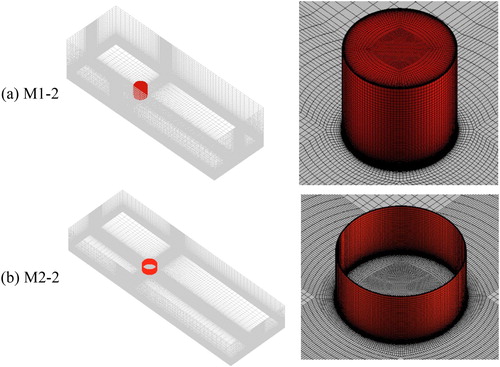
Table 2. A summary of the grid-independence test parameters.

Case	Number of grid nodes	H/D	b/D	SGS model	y/H	Re	y^+
M1-1	434,816	1	0.025	DSM	57%	2.9×10^5	0∼3.5
M1-2	1078,266	1	0.025	DSM	57%	2.9×10^5	0∼1.3
M1-3	1585,436	1	0.025	DSM	57%	2.9×10^5	0∼0.7
M1-4	1393,796	1	0.025	DSM	57%	2.9×10^5	0∼1.2
M2-1	1436,532	0.5	0.025	DSM	62%	2.5×10^5	0∼1.0
M2-2	2046,492	0.5	0.025	DSM	62%	2.5×10^5	0∼0.9
M2-3	4363,652	0.5	0.025	DSM	62%	2.5×10^5	0∼0.7
M2-4	4441,072	0.5	0.025	DSM	62%	2.5×10^5	0∼1.0

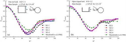
Figure 3 displays the time-averaged pressure coefficients (C_p,mean) on the flat roof and open-topped tank models computed from different meshes using LES and DSM SGS model, where the pressure coefficient C_p is defined as $C_p=2\left(p-p_{\mathrm{\infty }}\right)/\rho u_{\mathrm{\infty }}^2$. For the flat roof tank and open-topped tank, the wind pressures at y = 57%H and 62%H are sampled, respectively, and the numerical results are compared with the experimental results reported by Macdonald et al. (1988). As shown in Figure 3(a), for the flat roof tank, the wind pressure computed from mesh M1-2 is very close to those from the finer mesh (M1-3) and larger solution domain (M1-4), while the numerical results from the coarser mesh M1-1 deviate a lot from those from meshes M1-2, M1-3 and M1-4 in $\theta \in \left[{80}^{\circ },{135}^{\circ }\right]$. This indicates that sufficiently high grid density is necessary for LES. The pressure coefficients on the flat roof tank computed from M1-2, M1-3 and M1-4 agree well with the experimental data in most regions while deviate slightly in $\theta \in \left[{65}^{\circ },{95}^{\circ }\right]$ near the separation point. In the experiments of Macdonald et al. (1988), the tank is made of acrylic material and has surface roughness inevitably, which increases perturbation in the boundary layer, delays flow separation and promotes momentum transfer between the near-wall flow and main flow. Therefore, the wall pressures measured from the experimental tank model are higher than those computed from the smooth thank model used in the present numerical simulation. For the open-topped tank, similar results are obtained. As seen in Figure 3(b), the computed wind pressure coefficient from mesh M2-2 is very close to those from the finer mesh M2-3 and larger solution domain M2-4, while the numerical result from the coarser mesh M2-1 exhibits apparent discrepancy in $\theta \in \left[{120}^{\circ },{160}^{\circ }\right]$. Again, the wind loads computed from M2-2, M2-3 and M2-4 show a good agreement with the experiments.

Figure 3. Time-averaged pressure coefficients on the two tanks using different meshes: (a) flat roof tank, (b) open-topped tank.

To examine the effect of the SGS model on the numerical results from LES, turbulent flows around the flat roof tank and open-topped tank models are further simulated using mesh M1-2 and mesh M2-2, respectively, and SM, WALE and WMLES SGS models. Figure 4 presents the time-averaged wind pressure coefficients on the two tanks computed from different SGS models. As seen in the figure, when the SM SGS model is employed, the separation points on both tanks are moved forward a lot to $\theta \approx {\text{90}}^{\circ }$comparing with those observed in experiments and from the other SGS models. This deviation is associated with the pre-defined parameter C_s in the SM model, which has been found to introduce excessive damping to large-scale fluctuations in the presence of mean shear or in transitional flows near solid boundaries (Lilly, 1992). To solve this problem, in the DSM model C_s is computed dynamically based on the information provided by the resolved scales of flow motion. As a result, no excessive damping is generated and the separation points computed by the DSM SGS model agree very well with the experimental results. When the WALE and WMLES SGS models are used, the separation points of the two tanks models are also predicted correctly. However, the wind pressures computed from the WALE and WMLES models have larger discrepancies with the experimental results compared with those from the DSM model.

Figure 4. Time-averaged pressure coefficients on the two tanks from different SGS models: (a) flat-roof tank, (b) open-topped tank.

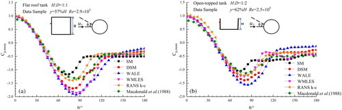
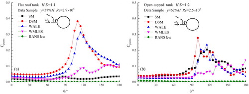
Figure 5 shows the root-mean-square of the instantaneous pressure coefficients relative to the time-averaged values, which indicates the oscillation of the wind pressure on each sample point. As shown in the figure, for both tank models the wind pressure on the windward side of the tank does not oscillate much. On the lee side of the tank, however, large oscillation of the wind pressure is observed due to the unsteady flow separation. The maximum pressure oscillation occurs near the separation point. Among four SGS models, the DSM SGS model attains the largest pressure oscillation, which means that this SGS model has the best sensitivity to the unsteadiness in the flow field. Therefore, the DSM SGS model is recommended when the LES method is applied to solve the turbulent flow around a tank.

Figure 5. Root-mean-square of the wind pressure coefficients on the two tanks from different SGS models: (a) flat-roof tank, (b) open-topped tank.

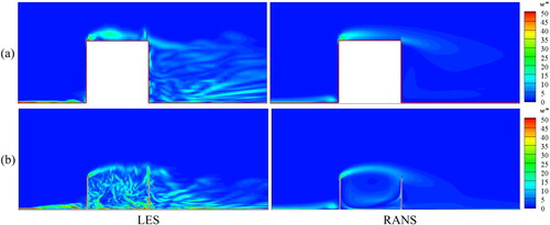
For the purpose of comparison, the numerical results computed from mesh M1-2 and mesh M2-2 using RANS with k-ε turbulence model are also presented in Figures 4 and 5. As seen in Figure 4, the time-averaged pressure coefficients computed from RANS have an overall good agreement with the experimental data, although it does not predict correctly the separation point of the flat-roof tank. As seen in Figure 5, however, the RANS method is a failure to simulate the unsteady oscillation of the wind pressure on the tank. To further compare the numerical results from RANS and LES, the instantaneous vorticity fields on the plane z = 0 are displayed in Figure 6. As shown in the figure, when the LES method is used, both large-scale and small-scale vortex structures are captured. When the RANS method is employed, however, the small-scale vortices are smoothed and the unsteady nature of the turbulence flow is not revealed. These results confirm the advantage of LES over RANS in simulating the unsteady turbulent flow around tanks.

Figure 6. Instantaneous vorticity fields around two tanks at t = 5 computed from LES and RANS: (a) flat-roof tank, (b) open-topped tank.

5. Numerical results and discussions

5.1 Computational model

Using LES with the DSM SGS model, the turbulent flow and wind load around an external floating-roof tank are further analyzed. The external floating-roof tank mainly consists of an open-topped cylindrical steel shell equipped with a flat roof that floats on the surface of the stored liquid. As the liquid level in the tank increases or decreases, the flat roof rises or falls accordingly. Taking the geometric scale of the 10⁵m³ external floating-roof tank used widely in oil strategic reserves into consideration, a simplified external floating-roof tank model is established. As shown in Figure 7, the external diameter of the tank is D, the height of the tank is H = 0.275D, and the maximum liquid level is H* = 0.25D. Considering the thickness of the floating roof is much smaller than H, the height of the top surface of the floating roof relative to the tank base is assumed equal to the liquid level h in the tank. To study effects of the liquid level and the Reynolds number, turbulent flows around this tank model at h = 25%H*, 50%H*, 75%H*, H* and Re = 5.47×10⁵, 1.09×10⁶, 1.64×10⁶, 2.19×10⁶ are simulated. The wall pressures at y = 2/3H of the external surface and y = h of the internal surface are sampled. For this tank model, the solution domain and boundary conditions are set the same with those used for the flat roof tank model as displayed in Figure 1, and the computational meshes are generated using the grid density similar with M1-2. Moreover, the turbulence intensity of the free stream is also set as 1.3%, which is the same as that in the experiments of Macdonald et al. (1988). Table 3 summaries the 16 simulating cases conducted for the external floating-roof tanks.

Figure 7. A schematic of the external floating-roof tank model at the maximum liquid level.

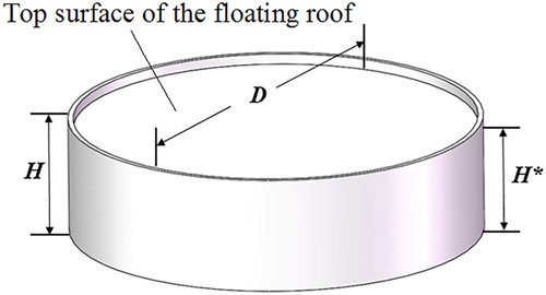
Table 3. A summary of the computations conducting for the external floating-roof tank.

				Re
Model	h/H*	Grid nodes	SGS	Case1	Case2	Case3	Case4
TANK 1	25%	2,101,168	DSM	5.47×10^5	1.09×10^6	1.64×10^6	2.19×10^6
TANK 2	50%	1,089,488	DSM	5.47×10^5	1.09×10^6	1.64×10^6	2.19×10^6
TANK 3	75%	1,058,368	DSM	5.47×10^5	1.09×10^6	1.64×10^6	2.19×10^6
TANK 4	100%	1,076,264	DSM	5.47×10^5	1.09×10^6	1.64×10^6	2.19×10^6

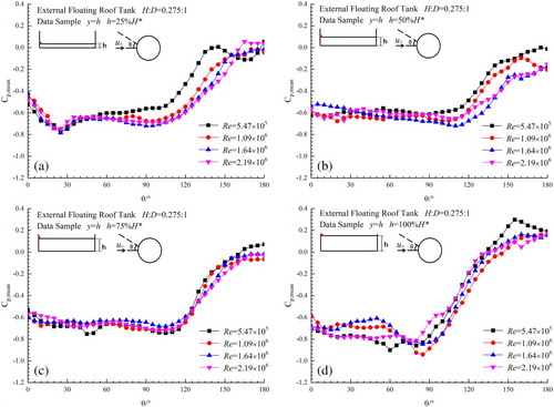
5.2. Effect of Reynolds number

Figure 8 compares the time-averaged pressure coefficients on the external wall of the tank at different Reynolds numbers. As seen in the figure, when the Reynolds number increases from 5.47×10⁵ to 1.09×10⁶, 1.64×10⁶ and 2.19×10⁶, the external wind loads of the tank at four liquid levels are not changed much on the windward side ($\theta \le {\text{90}}^{\circ }$) while increased slightly on the leeside (${\text{90}}^{\circ }\theta \le {180}^{\circ }$). Above Re = 10⁶, the pressure distribution on the external wall of the tank is almost independent of the Reynolds number. Figure 9 compares the time-averaged pressure coefficients on the internal wall of the tank at different Reynolds numbers. As seen in the figure, the wind load on the internal wall is essentially different from that on the external wall. At four liquid levels considered, the time-averaged wind pressures on the internal surface are negative in most regions and distributed more evenly than the external wind pressures. With the increase of θ from $0^{\circ }$ to ${180}^{\circ }$, the wind pressure on the internal wall is not changed much first while then increased when θ exceeds a critical value, which is reduced with the liquid level. At liquid levels of h = 25%H* and h = 50%H*, the internal pressures of the tank at higher θ drop a little bit at larger Reynolds numbers, while at h = 75%H* and 100%H* the internal pressures of the tank do not vary much with the Reynolds number, especially at Re > 10⁶.

Figure 8. Time-averaged pressure coefficients on the external wall of the tank at different Reynolds numbers: (a) h = 25%H*, (b) h = 50%H*, (c) h = 75%H*, (d) h = 100%H*.

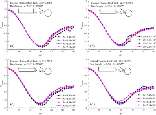
Figure 9. Time-averaged pressure coefficients on the internal wall of the tank at different Reynolds numbers: (a) h = 25%H*, (b) h = 50%H*, (c) h = 75%H*, (d) h = 100%H*.

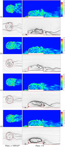
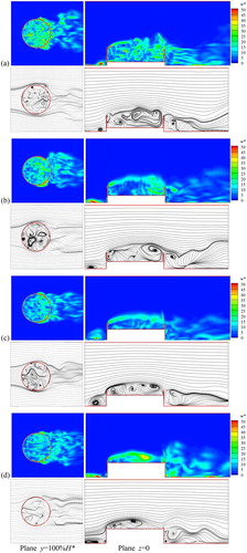
To show the effect of Reynolds number on the flow structures around the external floating-roof tank at low liquid level, Figure 10 displays the instantaneous vorticity fields and streamlines on the planes z = 0 and y = 100%H* at h = 25%H*. At the lower liquid level of h = 25%H*, a large cavity is formed above the roof of the tank. When airflow with lower speed (Re = 5.47×10⁵) is flowing around the tank, the flow is separated from the rim of the tank shell and many small-scale vortices are generated in the cavity, as shown in Figure 10(a). Considering there exists vortices on both of the z = 0 and y = 100%H* planes, the vortices in the cavity are three-dimensional. Moreover, vortices in the cavity have a larger scale on the plane z = 0 than on the plane y = 100%H*. Under the transport effect of these vortices, the pressure in the cavity is distributed more uniformly. Therefore, the wind pressure distribution on the internal wall of the tank is more uniform than that on the external wall, as seen in Figures 8(a) and 9(a). When the Reynolds number increases gradually from 5.47×10⁵ to 1.09×10⁶, 1.64×10⁶ and 2.19×10⁶, both strength and scale of the vortices in the cavity and around the tank are increased, as shown in Figure 10(b–d); in particular, the small-scale vortices in the cavity merge into a large one at higher Reynolds numbers, which makes the pressure on the internal wall distribute more uniformly, as seen in Figure 9(a).

Figure 10. Instantaneous vorticity fields and streamlines at t = 5 around the external floating-roof tank at h = 25%H* and different Reynolds numbers: (a) Re = 5.47×10⁵, (b) Re = 1.09×10⁶, (c) Re = 1.64×10⁶, (d) Re = 2.19×10⁶.

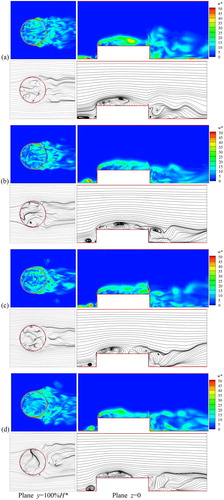
To study the effect of Reynolds number on the flow structures around the external floating-roof tank at high liquid level, Figure 11 displays the instantaneous vorticity fields and streamlines on the planes z = 0 and y = 100%H* at h = 100%H*. In this case, the cavity above the tank roof is very small and the roof is close to the main flow. As shown in Figure 11(a), when the airflow is flowing around the tank with maximum liquid level, the flow is separated from the front rim of the tank and then reattached to the roof near $\theta ={90}^{\circ }$. As a result, vortices are generated and evolved above the floating roof near the front rim of the tank and then shed into the downstream flow along the roof. In this process, the floating roof near the front rim of the tank is covered by vortices in most of the time. Therefore, the internal wind pressure is distributed more evenly in ${\text{0}}^{\circ }\le \theta \le {90}^{\circ }$, as shown in Figure 9(d). When the Reynolds number is increased from 5.47×10⁵ to 1.09×10⁶, 1.64×10⁶ and 2.19×10⁶, the strength of the vortices above and around the tank is increased gradually while the topology of the vortices is not changed much. Accordingly, the wind pressures on the external and internal walls of the external floating-roof tank at h = 100%H* are also not altered much, as shown in Figures 8(d) and 9(d).

Figure 11. Instantaneous vorticity fields and streamlines at t = 5 around the external floating-roof tank at h = 100%H* and different Reynolds numbers: (a) Re = 5.47×10⁵, (b) Re = 1.09×10⁶, (c) Re = 1.64×10⁶, (d) Re = 2.19×10⁶.

5.3. Effect of liquid level

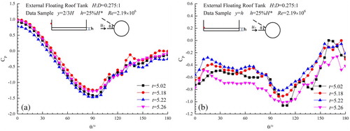
Figures 12 and 13 illustrate variations of the time-averaged pressure coefficients on the external and internal walls of the external floating-roof tank with respect to the liquid level, respectively. As the effect of the Reynolds numbers on the wind loads is very small at Re > 10⁶, only the numerical results at Re = 5.47×10⁵ and Re = 2.19×10⁶ are presented. As seen in Figure 12, the wind pressure on the external wall of the tank is not influenced much by the liquid level in the tank (position of the floating roof). The wind pressure on the internal wall of the tank, however, is affected significantly by the liquid level. As shown in Figure 13, the internal wind pressure at h = 100%H* is very different from that at h = 75%H*, 50%H* and 25%H*. At h = 100%H*, the pressure on the internal wall surface is lower near the front rim of the tank while higher near the back rim of the tank, than those at the lower liquid levels. Moreover, at h = 100%H* the region where the internal wall pressure is distributed quite evenly is $\theta \le {90}^{\circ }$, while at h = 75%H*, 50%H* and 25%H* the corresponding region is $\theta \le {120}^{\circ }$. This indicates that the pressure distribution on the floating roof is more nonuniform near the full liquid level, which raises the risk of roof inclination. Figure 14 displays the instantaneous wall pressure coefficients of the external floating-roof tank at 25%H* and Re = 2.19×10⁶. Because the flow around the tank is highly turbulent, the wall pressure of the tank oscillates significantly. Comparing Figure 14(a) with Figure 14(b), it can be found that the inner wall above the roof has much larger pressure oscillation than the external wall. This indicates that the cylindrical shell above the floating roof experiences significantly oscillating wind load, which could lead to vibration or fatigue of the structure.

Figure 12. Time-averaged pressure coefficients on the external wall of the tank at different liquid levels: (a) Re = 5.47×10⁵, (b) Re = 2.19×10⁶.

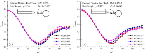
Figure 13. Time-averaged pressure coefficients on the internal wall of the tank at different liquid levels: (a) Re = 5.47×10⁵, (b) Re = 2.19×10⁶.

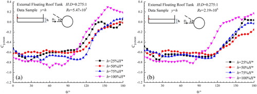
Figure 14. Instantaneous wall pressure coefficients of the tank at h = 25%H* and Re = 2.19×10⁶: (a) external wall, (b) internal wall.

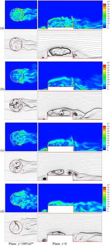
To understand the effect of the liquid level on the wind loads on the external floating-roof tank, Figures 15 and 16 display the instantaneous vorticity fields and streamlines on the planes z = 0 and y = 100%H* at Re = 5.47×10⁵ and Re = 2.19×10⁶, respectively. As shown in Figure 15, at Re = 5.47×10⁵ the flow structure around the tank does not change much with the liquid level, resulting in similar pressure lines on the external wall surface at different liquid levels, as shown in Figure 12(a). In the cavity above the tank, however, the situation is somewhat different. As shown in Figure 15(a), the cavity above the roof is filled with small vortices at the low liquid level of h = 25%H*, which generates the uniform distribution of the internal pressure. With an increase of the liquid level from h = 25%H* to 50%H* and 75%H*, the volume of the cavity above the floating roof is decreased continuously. Although the number of vortices in the cavity above the roof is decreased, the whole cavity is still covered by vortices, as seen in Figure 15(b and c). Therefore, the wind pressure distributions on the internal wall at h = 50%H* and 75%H* are similar with that at h = 25%H* as presented in Figure 13(a). At h = 100%H*, however, vortices no longer fill the whole cavity but only cover the region near the front rim of the tank, as seen in Figure 15(d). This has resulted in the apparent change of the pressure distribution on the internal wall at h = 100%H*, as shown in Figure 13(a).

Figure 15. Instantaneous vorticity fields and streamlines at t = 5 around the external floating-roof tank at Re = 5.47×10⁵ and different liquid levels: (a) h = 25%H*, (b) h = 50%H*, (c) h = 75%H*, (d) h = 100%H*.

At high Reynolds number of 2.19×10⁶, the effect of liquid level on the flow field of the external floating-roof tank is similar with that at Re = 5.47×10⁵. As shown in Figure 16, the flow structure around the tank does not vary much with the liquid level. Therefore, the wind loads on the external wall of the tank are similar at different liquid levels as seen in Figure 12(b). In the cavity above the floating roof, a large-scale vortex is formed at h = 25%H*, which makes the wind pressure on the internal wall surface distributed uniformly in $\theta \le {120}^{\circ }$, as seen in Figures 16(a) and 13(b). When the liquid level rises from 25%H* to 50%H* and 75%H*, the large-scale vortex is split into several smaller ones, as shown in Figure 16(b and c). However, because the cavity is still filled with vortices, this change in flow structure does not bring remarkable influence on the wind pressure on the internal wall at h = 50%H* and 75%H*, as shown in Figure 13(b). At h = 100%H*, again, the region in the cavity which is always covered by vortices shrinks as seen in Figure 16(d), which decreases the area with uniform pressure distribution on the internal wall as shown in Figure 13(b).

Figure 16. Instantaneous vorticity fields and streamlines at t = 5 around the external floating-roof tank at Re = 2.19×10⁶ and different liquid levels: (a) h = 25%H*, (b) h = 50%H*, (c) h = 75%H*, (d) h = 100%H*.

6. Conclusions

Using large eddy simulation with high accuracy, effects of Reynolds number and liquid level on the flow structure and wind load of an external floating-roof tank model are investigated numerically. Based on the numerical results obtained, several conclusions can be made as follows:

1. The RANS method with k-ε turbulence model is capable of solving the time-averaged wind pressure on the tank but is unable to compute the pressure oscillation and small-scale vortex structures, while the LES method is able to describe both of the time-averaged and transient flow features.

2. When LES is employed to compute the flow field and wind pressure of a tank, the DSM subgrid-scale eddy viscosity model has a better performance than the SM, WALE and WMLES subgrid-scale eddy viscosity models.

3. With the increase of the Reynolds number, the strengths of vortices in the cavity above the floating roof and around the tank are increased while the topologies of these vortices are not altered significantly. Therefore, the wind pressure coefficients on the external and internal walls of an external floating-roof tank are not changed much with the Reynolds numbers, especially at Re > 10⁶.

4. The liquid level has a great effect on the flow field and wind load of an external floating-roof tank. At lower liquid levels, the cavity above the floating roof of the tank is filled with vortices, which makes the wind pressure on the internal wall distribute uniformly in $\theta \le {120}^{\circ }$. Near the full liquid level, the vortices generated from the front rim reattach to the roof and only part of the roof is always covered by vortices, which reduces the region on the internal wall where the wind pressure is distributed evenly.

As our first attempt at applying LES to the flow around a tank, only the wind load and the vortex structure of the external floating-roof tank are focused, while the response of the structure components such as the floating roof and cylindrical shell is not considered. Based on wind loads and flow structures obtained, responses of the structure components and dissipation of the oil vapor from the roof seal can be estimated qualitatively. Additionally, considering the transient, not time-averaged, flow field can be solved by LES, the LES solver presented here can be further combined with the structural solvers concerning static deformation, buckling or vibration, to assess the structure safety of a tank in strong wind.

Acknowledgements

The authors would like to thank for the kind support of the two fundings.

Disclosure statement

No potential conflict of interest was reported by the author(s).

Additional information

Funding

This work is supported by the National Key Research and Development Program of China (No.2017YFC0805801) and the National Natural Science Foundation of China (No.51374224).

References

- Acheinbach, E. (1968). Distribution of local pressure and skin friction around a circular cylinder in cross-flow up to Re = 5×10⁶. Journal of Fluid Mechanics, 34, 625–669. doi: 10.1017/S0022112068002120
- Achenbach, E. (1972). Experiments on flow past spheres at very high Reynolds numbers. Journal of Fluid Mechanics, 54, 565–575. doi: 10.1017/S0022112072000874
- Akbarian, E., Najafi, B., Jafari, M., Ardabili, S. F., Shamshirband, S., & Chau, K. W. (2018). Experimental and CFD-based numerical simulation of using natural gas in a dual-fuelled diesel engine. Engineering Applications of Computational Fluid Mechanics, 12(1), 517–534. doi: 10.1080/19942060.2018.1472670
- Ardabili, S. F., Najafi, B., Shamshirband, S., Bidgoli, B. M., Deo, R. C., & Chau, K. W. (2018). Computational intelligence approach for modeling hydrogen production: A review. Engineering Applications of Computational Fluid Mechanics, 12(1), 438–458. doi: 10.1080/19942060.2018.1452296
- Erlebacher, G. (1990). Toward the large-eddy simulation of compressible turbulent flows. Journal of Fluid Mechanics, 238, 155–185. doi: 10.1017/S0022112092001678
- Falcinelli, O. A., Elaskar, S. A., & Godoy, L. A. (2011). Influence of topography on wind pressures in tanks using CFD. Latin American Applied Research, 41(4), 379–388.
- Germano, M., Piomelli, U., Moin, P., & Cabot, W. H. (1991). A dynamic subgrid-scale eddy viscosity model. Physics of Fluids A: Fluid Dynamics, 3, 1760–1765. doi: 10.1063/1.857955
- Ghalandari, M., Koohshahi, E. M., Mohamadian, F., Shamshirband, S., & Chau, K. W. (2019). Numerical simulation of nanofluid flow inside root canal. Engineering Applications of Computational Fluid Mechanics, 13(1), 254–264. doi: 10.1080/19942060.2019.1578696
- Godoy, L. A. (2007). Performance of storage tanks in oil facilities following hurricanes Katrina and Rita. ASCE Journal Performance of Constructed Facilities, 21(6), 441–449. doi: 10.1061/(ASCE)0887-3828(2007)21:6(441)
- Greiner, R., & Derler, P. (1995). Effect of imperfections on wind-loaded cylindrical shells. Thin-Walled Structures, 23(1–4), 271–281. doi: 10.1016/0263-8231(95)00016-7
- Hannat, R., Weiss, J., Garnier, F., & Morency, F. (2014). Application of the dual Kriging method for the design of hot-air-based aircraft wing anti-icing system. Engineering Applications of Computational Fluid Mechanics, 8(4), 530–548. doi: 10.1080/19942060.2014.11083305
- Hinze, J. O. (1975). Turbulence. New York: McGraw-Hill.
- Holroyd, R. J. (1983). On the behaviour of open-topped oil storage tanks in high winds, Part I. Aerodynamic aspects. Journal of Wind Engineering and Industrial Aerodynamics, 12, 329–352. doi: 10.1016/0167-6105(83)90054-5
- Lilly, D. K. (1992). A proposed modification of the Germano subgrid-scale closure method. Physics of Fluids A: Fluid Dynamics, 4(4), 633. doi: 10.1063/1.858280
- Lin, Y., & Zhao, Y. (2014). Wind loads on fixed-roof cylindrical tanks with very low aspect ratio. Wind and Structures: An International Journal, 18(6), 651–668. doi: 10.12989/was.2014.18.6.651
- Macdonald, P. A., Kwok, K. C. S., & Holmes, J. D. (1988). Wind loads on circular storage bins, silos and tanks: Point pressure measurements on isolated structures. Journal of Wind Engineering and Industrial Aerodynamics, 31, 165–188. doi: 10.1016/0167-6105(88)90003-7
- Montazeri, H., & Blocken, B. (2013). CFD simulation of wind-induced pressure coefficients on buildings with and without balconies: Validation and sensitivity analysis. Building and Environment, 60(2), 137–149. doi: 10.1016/j.buildenv.2012.11.012
- Mou, B., He, B. J., Zhao, D. X., & Chau, K. W. (2017). Numerical simulation of the effects of building dimensional variation on wind pressure distribution. Engineering Applications of Computational Fluid Mechanics, 11(1), 293–309. doi: 10.1080/19942060.2017.1281845
- Mulhearn, P. J., Banks, H. J., Finnigan, J. J., & Annis, P. C. (1976). Wind forces and their influence on gas loss from grain storage structures. Journal of Stored Products Research, 12(3), 129–142. doi: 10.1016/0022-474X(76)90001-1
- Murakami, S., & Mochida, A. (1995). On turbulent vortex shedding flow past 2D square cylinder predicted by CFD. Journal of Wind Engineering and Industrial Aerodynamics, 54–55, 191–211. doi: 10.1016/0167-6105(94)00043-D
- Nicoud, F., & Ducros, F. (1999). Subgrid-scale stress modeling based on the square of the velocity gradient tensor. Flow Turbulence & Combustion, 62(3), 183–200. doi: 10.1023/A:1009995426001
- Pasley, H., & Clark, C. (2000). Computational fluid dynamics study of flow around floating-roof oil storage tanks. Journal of Wind Engineering and Industrial Aerodynamics, 86(1), 37–54. doi: 10.1016/S0167-6105(99)00138-5
- Pope, S. (2000). Turbulent flows. Cambridge: Cambridge University Press.
- Portela, G., Virella, J. C., & Godoy, L. A. (2006). Buckling of unanchored tanks under wind. XXIII South Eastern Conference on Theoretical and Applied Mechanics, Puerto Rico, pp. 167–176.
- Probert, S. D., Hasoon, M. A., & Lee, T. S. (1973). Boundary layer separation for winds flowing around large fixed-roof oil-storage tanks with small aspect ratios. Atmospheric Environment, 7(6), 651–654. doi: 10.1016/0004-6981(73)90022-X
- Ramezanizadeh, M., Nazari, M. A., Ahmadi, M. H., & Chau, K. W. (2019). Experimental and numerical analysis of a nanofluidic thermosyphon heat exchanger. Engineering Applications of Computational Fluid Mechanics, 13(1), 40–47. doi: 10.1080/19942060.2018.1518272
- Shur, M. L., Spalart, P. R., Strelets, M. K., & Travin, A. K. (2008). A hybrid RANS-LES approach with delayed-DES and wall-modelled LES capabilities. International Journal of Heat and Fluid Flow, 29, 1638–1649. doi: 10.1016/j.ijheatfluidflow.2008.07.001
- Smagorinsky, J. (1963). General circulation experiments with the primitive equations. Monthly Weather Review, 91(3), 99–164. doi: 10.1175/1520-0493(1963)091<0099:GCEWTP>2.3.CO;2
- Tominaga, Y., Mochida, A., Yoshie, R., Kataoka, H., Nozu, T., Yoshikawa, M., & Shirasawa, T. (2008). AIJ guidelines for practical applications of CFD to pedestrian wind environment around buildings. Journal of Wind Engineering and Industrial Aerodynamics, 96, 1749–1761. doi: 10.1016/j.jweia.2008.02.058
- Uematsu, Y., Koo, C., & Yasunaga, J. (2014). Design wind force coefficients for open-topped oil storage tanks focusing on the wind-induced buckling. Journal of Wind Engineering and Industrial Aerodynamics, 130, 16–29. doi: 10.1016/j.jweia.2014.03.015