Hydraulic transport flow law of natural gas hydrate pipeline under marine dynamic environment

Abstract

The work simulates the transport pipeline movement of the marine dynamic environment based on the computational fluid dynamics research method. The present work also studies the influence of the marine dynamic environment on the solid–liquid two-phase flow field in the pipeline. An experimental study on the hydraulic transport flow law of natural gas hydrate pipeline is performed on the experimental platform of deep-sea mining metallogenic system fluctuation. Results show a large disturbance of the transverse swing convection field of pipelines and a small influence of axial vibration. The flow field distribution characteristics in the conveyor pipeline are consistent with the steady-state working conditions when the amplitude of transverse oscillation is less than 0.5 m. When the oscillation amplitude is larger than 2 m, the vibration has a considerable influence on the solid-phase distribution, solid–liquid two-phase velocity, dynamic and static pressure, and pressure loss of the flow field in the conveying system. The flow field distribution is chaotic when the transverse oscillation period of the pipeline is small. This condition becomes highly evident when the oscillation amplitude is large. 

KEYWORDS:

• Marine dynamic environment
• natural gas hydrate
• hydraulic conveying
• flow law
• CFD

1. Introduction

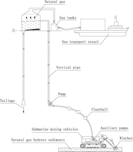
Natural gas hydrates are regarded as promising new energy sources because of their wide distribution and large reserves on earth. Moreover, the burning of natural gas does not produce harmful gases similar to fossil fuels. At present, the suction mining method is the most promising method for the commercial exploitation of submarine natural gas hydrate. However, the core problem of this method lies in the hydraulic conveying of solid particles through the pipeline (Zou & Huang, 2006). In mining systems, vertical pipelines are complex under the influence of dynamic environmental factors, such as current, wave, machine movement collection, and mining vessel tug (Osorio, Ortega, & Arango-Aramburo, 2015). Thus, simulating the marine dynamic environment via experiment or simulation is difficult. Figure 1 shows a sketch of the natural gas hydrate mining system.

Figure 1. Brief map of natural gas hydrate mining systems.

The current research results in this field mainly include the following. Felippa & Chung(1981) statically analyzed pipeline deformation under the action of gravity, sea flow force, fluid force in the tube, and mining ship towing by using a nonlinear finite element model. Chung (1998) conducted a transient analysis of the vertical vibration of the ore pipeline. Wang, Liu, Abdelkefi, Wang, and Dai (2017) established the 5000 m deep-sea conveying pipeline model by using finite element analysis software. They also analyzed the geometrical nonlinear static and dynamic characteristics of deep-sea mining pipes under the influence of dynamic environmental factors, such as wave, current, and mining ship towing. Their results demonstrate the production of a large offset through the deep-sea mining tube under the action of ocean dynamics, and the offset distance is related to the environment.

Liu, Hu, and Dai (2017) established the fluid–solid coupling model of deep-sea mining conveying hose and studied the variation law of the spatial configuration of conveyor hose under the influence of ocean power and mining. They also developed a fluid–solid coupling model for the hard tubes and outflows of deep-sea mining mines to analyze the influence of ocean dynamics on the transverse migration of conveying pipelines by using the finite element method. Payne, Kiprakis, Ehsan, Rampen, and Wallace (2007), Camenen (2007), and Song, Xiao, and Feng (2010) summarized the results of the existing research and found that the transverse oscillation amplitude of deep-sea mining pipelines under the action of ocean power is 0.7–110 m and the transverse oscillation period is 1.25–120 s. The influence of transverse oscillation and axial vibration of conveying pipelines on their pressure loss slope is studied via testing. Pei, Wang, and Yuan (2014) combined experimental and theoretical analyses and concluded that the pressure loss is larger than the static state when the pipeline swings but obtained no specific influence law.

Overall, studies on the marine dynamic environment of the deep-sea mining pipeline transport mainly involving the transport pipeline space configuration, overall migration, and other issues regarding the marine dynamic environment on the flow field of the conveyor pipeline research are limited. In the present work, the combination of numerical simulation and experimental research will be used to analyze the influence of deep-sea ore transportation systems on fluid flows in pipelines under the marine dynamic environment.

To study the influence of marine dynamic environment on the internal flow field of natural gas hydrate pipeline transmission. Firstly, the paper construct a numerical model of the analysis field of the internal flow field in the pipeline. Then, the influences of different vibration conditions on the solid phase concentration of the pipeline outlet, the solid phase distribution of the flow field in the pipeline, the velocity distribution and the pressure loss are numerically simulated. On the basis of numerical simulation, the numerical results are verified by means of the marine dynamic environment simulation wave experiment platform.

Under the marine dynamic environment, due to the non-directional oscillation of the pipeline, there is a high coupling between the momentum equation of the fluid in the pipeline, and the internal flow field is prone to a large pressure gradient. It makes the vortex redistribution in the flow field. These couplings easily lead to the instability of the calculation process. In order to avoid the above problems, the method of coupling non-steady state solution is used in numerical simulation, the velocity subslack factor is reduced, and the multiphase flow is defined as the Mixture model.

In addition, when Computational Fluid Dynamics (CFD) numerically simulates the flow field in a oscillating pipe, there is a lack of relevant modules that externally excited vibrations are applied to the flow field. The paper intends to use the C language and the Define macro command provided by CFD to write the program required for externally excited vibration to be applied to the flow field (that is, UDF program, UDF is the abbreviation of User-Defined Function). Use the macro commands provided by the CFD user-defined function to specify the motion area of the mesh. Write a transient Profile file to specify the motion mode for the motion area. In the numerical simulation, the UDF program and the analysis data are passed to the solver, and the CFD solver dynamically loads it to complete the simulation calculation.

2. Geometric model and kinematic condition

2.1. Geometric models

The working condition of 4500 m sea depth is used as the research object in this study. Simulating the full length of the pipe is inconvenient because the entire conveying system is long; the slurry enters the pipeline at a certain distance to reach a stable conveying state, and the flow field law remains unchanged after entering the stable state (Xu, Chen, Wu, & Yang, 2016). Therefore, one of these factors can be intercepted for study in numerical calculation.

The pipe diameter (0.3 m) of the conveyor pipeline is used as the research representative to determine the appropriate length of the simulation model. The pipeline models with lengths of 10, 15, 20, and 30 m are intercepted, and the same method is used to divide the pipelines with different lengths. The actual working conditions indicate that the slurry flow rate at the entrance is 2 m/s, the particle size is 20 mm, and the volume concentration is 0.1 kg/L. The four models are used to simulate and analyze the same working condition.

Table 1 and Figure 2 show the numerical results. Table 1 is the solid-phase average concentration and solid–liquid two-phase velocity at the outlet of the four models. Figure 2 shows the solid-phase velocity distribution at the outlet of the four model pipelines.

Figure 2. Comparison of solid-phase outlet velocity of the fourpipeline model lengths.

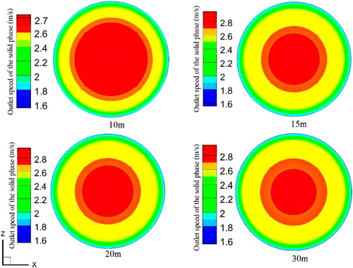
Table 1. Comparison of export parameters of the four pipeline model lengths.

Model length/m	10	15	20	30
Average outlet concentration of solid phase/(kg/L)	0.11274	0.11286	0.11299	0.11291
Average outlet speed of solid phase/(m/s)	2.72453	2.72362	2.72349	2.72225
Average outlet speed of liquid phase/(m/s)	3.14776	3.14453	3.14875	3.14986

Table 1 demonstrates the similarity of the simulation results of the four models. Compared with the solid-phase velocity distribution in Figure 2, the distribution law of solid-phase velocity of the four models is similar. Consequently, the annular distribution decreases from the center of the circle to the circumference. Further analysis shows that the maximum velocity of the solid phase of the 10 m model is 2.7 m/s, and the maximum speed of 15, 20, and 30 m models is 2.4 m/s. The solid-phase velocity distribution of 15, 20, and 30 m models is the same, and the solid-phase velocity of the 10 m model is quite different. The area of the central high-speed area on the outlet surface of the 10 m model is significantly larger than that of 15, 20, and 30 m models. This finding shows that the flow field in the 0–10 m flow section of the slurry has not been fully developed and has not reached a stable state. By contrast, the flow field in the 10–15 m flow section is gradually stable and remains unchanged after 20 m.

Considering the calculation time and accuracy requirements, the selection of the 20 m pipeline model as the research object is studied in this paper.

2.2. Kinematic equation

The movement state of submarine gas hydrate pipelines under the action of the marine dynamic environment is complicated (Ihle, 2013). The conveyor pipeline is assumed to have a simple harmonic motion under the action of the marine dynamic environment. This assumption facilitates the effective use of the dynamic mesh model of CFD software for the moving state simulation of pipelines.

The distance–time function of motion is: (1) $s=A\cdot \cos \left(\frac{2\pi }{T}t+\pi \right).$(1) The speed–time function of motion is: (2) $v=\frac{2\pi A}{T}\cdot \sin \left(\frac{2\pi }{T}t\right).$(2) The acceleration–time function of motion is: (3) $a=\frac{4{\pi }^{2}A}{T^2}\cdot \cos \left(\frac{2\pi }{T}t\right).$(3) In formulas (1)–(3), s is the moving distance, m; v is the movement speed, m/s; a is the motion acceleration, m/s²; A is the motion amplitude, m; T is the motion period, s; and t is the time, s.

When the flow field in the conveyor pipeline is numerically simulated in the marine dynamic environment, no external excitation vibration is applied to the correlation module of the flow field in the CFD interface(Mohebbi & Behbahani, 2014; Rajnauth & Barrufet, 2012; Ramezanizadeh, Alhuyi Nazari, Ahmadi, & Chau, 2019; Van Wijk, Talmon, & Van Rhee, 2016). The article uses the C language and combines the defined macro-commands provided by CFD to write the required program (UDF). The motion area of the grid is identified through the DEFINE_ZONE_MOTION command provided by the CFD user custom function, and the transient profile file is written to specify the motion mode for the motion area(Mosavi, Shamshirband, Salwana, Chau, & Tah, 2019). In the numerical calculation, the UDF program and data are passed to the solver, and the CFD Solver completes the required calculation in this study after dynamic loading.

3. Numerical simulation

3.1. Control equations

A relative slip is observed between the solid–liquid two-phase control field in the pipeline of natural gas hydrate. This slip indicates a strong interaction due to the action of gravity. The Eulerian model in the multiphase flow model is selected for numerical simulation. The solid–liquid two-phase flow control equation based on the Eulerian model mainly includes continuity and momentum equations (Li, Xu, & Yang, 2015; Makogon, 2010; Wu, Wang, Liu, & Xu, 2015).

1. Liquid-phase control equation

Continuous equations: (4) $\frac{\mathrm{\partial }(1-{\phi }_v)}{\mathrm{\partial }t}+\frac{\mathrm{\partial }[(1-{\phi }_v){\mathbf{\text{u}}}_{\mathbf{\text{li}}}]}{\mathrm{\partial }{x}_i}=0.$(4) Momentum equation: (5) $\begin{array}{rl}& \frac{\mathrm{\partial }}{\mathrm{\partial }t}[(1-{\phi }_v){\mathbf{\text{u}}}_{\mathbf{\text{l}}}]+\mathrm{\nabla }\cdot [(\text{1}-{\phi }_v){\mathbf{\text{u}}}_{\mathbf{\text{l}}}{\mathbf{\text{u}}}_{\mathbf{\text{l}}}]=(\text{1}-{\phi }_v)F_{\text{l}}\\ & -\frac{1}{{\rho }_{\text{l}}}\mathrm{\nabla }\cdot [(\text{1}-{\phi }_v)P]+\frac{1}{{\rho }_{\text{l}}}\mathrm{\nabla }\cdot [(\text{1}-{\phi }_v){\mathit{\tau }}_{\mathbf{\text{l}}}]+\frac{M_{\text{l}}}{{\rho }_{\text{l}}},\end{array}$(5) Where ${\phi }_v$ is the solid-phase volume concentration, u_l is the liquid-phase velocity vector, ${\rho }_{\text{l}}$ is the liquid phase density, τ_l is the stress tensor of the liquid phase, $F_1$ is the external force of the liquid phase unit mass, $M_{\text{l}}$ is the interphase force, and P is the equivalent pressure.

1. (2) Solid-phase control equation

Continuity equation: (6) $\frac{\mathrm{\partial }{\phi }_v}{\mathrm{\partial }t}+\frac{\mathrm{\partial }{\phi }_{\text{v}}{\mathbf{\text{u}}}_{\mathbf{\text{si}}}}{\mathrm{\partial }{x}_i}=0.$(6) Momentum equation: (7) $\begin{array}{rl}& \frac{\mathrm{\partial }}{\mathrm{\partial }t}({\phi }_v{\mathbf{\text{u}}}_s)+\mathrm{\nabla }\cdot ({\phi }_v{\mathbf{\text{u}}}_s{\mathbf{\text{u}}}_s)\\ & ={\phi }_v{F}_s-\frac{1}{{\rho }_s}\mathrm{\nabla }\cdot ({\phi }_{v}P)+\frac{1}{{\rho }_s}\mathrm{\nabla }\cdot ({\phi }_v{\mathit{\tau }}_s)+\frac{M_s}{{\rho }_s},\end{array}$(7) Where u_s is the solid-phase velocity vector, ρ_s is the solid phase density, τ_s is the stress tensor affected by the solid phase, F_s is the external force of the solid-phase unit mass, and M_s is the interphase force.

The interaction force of solid–liquid two-phase control flow field belongs to the internal force in the mixed fluid according to the principle of force and reaction: (8) $M_{\text{l}}+M_s=0.$(8)

3.2. Grid partitioning

The types of mesh division include structured and unstructured meshes, which have good quality and high calculation accuracy and efficiency. The lifting pipeline studied in this work is cylindrical, and the structure is regular; thus, the use of structured mesh is beneficial to the rapid convergence of calculation results (Eivaz et al., 2018; Mou, He, Zhao, & Chau, 2017; Yuliang, Yi, Baoling, Zuchao, & Huashu, 2013).

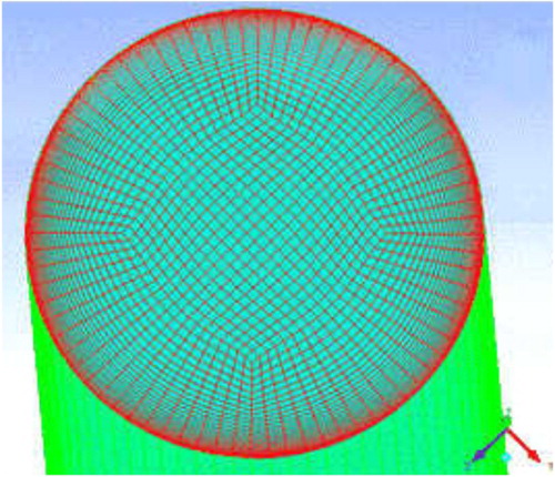
Figure 3 shows that the ICEM grid partitioning tool uses O-type segmentation to divide the pipeline model in a structured grid using the Exponential 1 distribution law to encrypt the boundary layer mesh (Ghalandari, Mirzadeh Koohshahi, Mohamadian, Shamshirband, & Chau, 2019; Wang,2016).

Figure 3. Structured grid of the three-dimensional pipeline model.

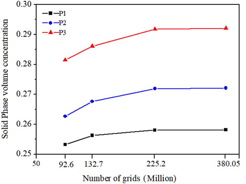
Four types of sizes were used to divide the pipeline model to verify the influence of mesh size on the calculation results. The corresponding mesh numbers were 92.6, 132.7, 225.2, and 380.0.5 million. The solid-phase concentration monitoring is performed at three points from the pipeline inlet 10 and 12.5 m in the model by using four types of meshes to simulate and analyze the same working condition. The specific coordinates of the three points are P1 (0,1000,75), P2 (0,12500,0), and P3 (0,12500,−75). Figure 3 demonstrates the relationship between the solid-phase volume concentration and the number of meshes at three monitoring points.

Figure 4 shows an increasing trend in the solid-phase volume concentration of each monitoring point with the number of model meshes. The solid-phase volume concentration of the three monitoring points considerably increased when the number of meshes increased from 92.6 million to 132.7 million. By contrast, the number of meshes increased from 132.7 million to 380.05 million, and the increase in solid-phase volume concentration was small in three monitoring points. From the viewpoint of calculation accuracy and time cost, this work selects the mesh type with a mesh number of 225.2 million for numerical simulation.

Figure 4. Grid size-independent validation results.

4. Result analysis

4.1. Effect of transverse oscillation amplitude on solid-phase average concentration of pipeline outlets

The lifting pipe will produce transverse oscillation under the influence of the marine dynamic environment. Considering the calculation time and space requirements, the setting oscillation amplitude is analyzed under six types of working conditions of A at 0.25, 0.5, 1, 2, 4, and 10 m. The calculation time is 40 s.

The slurry inside the pipe is in a stable conveying state before the addition of the swing load, and the swing load is added from t = 0 s. Figure 5 shows that the change in the solid-phase average volume concentration of the conveying pipeline outlet under six swing ranges exceeds the time. The solid-phase average concentration of the pipeline outlet is stable in the first period. The stability times corresponding to 0.25, 0.5, 1, 2, 4, and 10 m are 6, 5, 4, 3, 2, and 2 s, respectively. The influence on the fluid in the tube is remarkable when the swing is large. Afterward, the outlet concentration showed periodic fluctuation, and the change period was 10 s, which was half of the pipeline oscillation period. This phenomenon is due to the same effect of the pipe movement along the positive and negative directions on the flow field in the tube.

Figure 5. Variations of solid-phase average volume concentrations of pipeline outlets under different swing conditions when the swing period is 40 s. (a) Swing amplitude 0.25 m. (b) Swing amplitude 0.5 m. (c) Swing amplitude 1 m. (d) Swing amplitude 2 m. (e) Swing amplitude 4 m. (f) Swing amplitude 10 m.

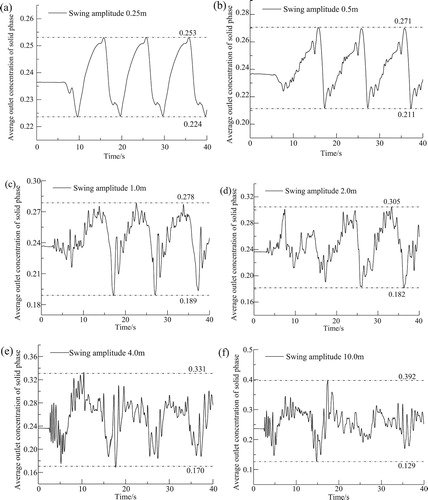
The maximum outlet concentrations of the solid phase were 0.253, 0.271, 0.278, 0.305, 0.331, and 0.392, and the variation amplitudes of the outlet concentrations were 0.029, 0.06, 0.089, 0.123, 0.161, and 0.263, respectively. Thus, the change in export concentration is intense when the swing is large. When the pendulum does not exceed 1 m, the pipeline outlet concentration demonstrates minimal changes. The difference between maximum outlet concentrations and steady-state conditions is only approximately 0.04. When the pendulum exceeds 0.4 m, the maximum volume concentration of the outlet nearly reaches the limit conveying concentration, which easily causes plugged pipes. When the amplitude is 0.25 m, the change in outlet concentration demonstrates a smooth curve. The change curve of the outlet concentration becomes jagged with the increase in the swing amplitude.

The pipeline undergoes acceleration and deceleration processes during the harmonic swing process. The solid-phase particles in the inertial action will collide with the pipe wall and adjacent solid-phase particles and produce the aggregation phenomenon, resulting in the uneven distribution of solid particles in the tube. A large swing amplitude leads to chaotic solid-phase particle distributions in the inner slurry and substantial changes in solid-phase concentration at the pipeline outlet.

4.2. Effect of transverse oscillation of pipeline on solid-phase distribution

The solid-phase particles collide with the pipe wall and produce aggregation due to inertial action during the oscillation process. This collision will lead to the uneven distribution of solid particles in the tube. High concentrations of solid particles in the pipeline will affect the efficiency of the system and even produce the reflux phenomenon. The distribution of solid-phase particles in the pipeline outlet and pipeline at different times is studied by selecting the transverse oscillation period of 20 s and the working condition of 2 m.

Figures 6 and 7 are the distributions of solid-phase particles on the XOY plane of the tube and at the pipe outlet under steady and transient conditions, respectively. Figure 6 demonstrates that the solid-phase particles accumulate at approximately 1 m away from the inlet after the entrance of the slurry in the pipeline under steady-state conditions, and the maximum solid concentration reaches 0.34. Afterward, the solid-phase distribution slightly changes under the push of the liquid phase upward movement but remains uniform. The concentration between 0.26 and 0.28 is higher than the import concentration. This condition is attributed to the relative sliding between the solid–liquid two-phase flow under the action of gravity. Thus, this phenomenon leads to a certain accumulation of solid-phase particles in the conveying process.

Figure 6. Solid-phase distribution of the XOY surface in the tube at different times when the period is 20 s and the oscillation amplitude is 2 m.

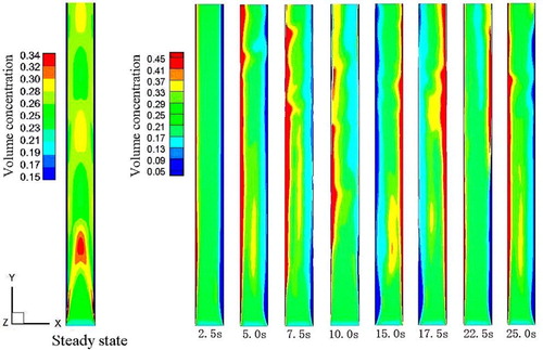
Figure 7. Solid-phase distribution of the pipeline outlet at different times when the period is 20 s and the oscillation amplitude is 2 m.

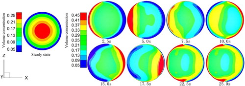
Figure 7 indicates that the solid phase has a circular distribution in the pipeline interface, thereby showing a state of high intermediate and low peripheral concentrations. This condition is attributed to the higher flow rate in the middle of the flow field in the slurry conveying process than the surrounding flow rate, which will produce a radial force on the solid-phase particles; accordingly, the solid-phase particles will gather into the center of the pipeline.

The figure also shows that the distribution of the solid phase in the tube changes with time after the motion load application, and the maximum concentration reaches 0.45. The solid-phase agglomeration degree is more serious than the steady-state working condition. In t = 0–5 s, the pipeline accelerates to the right, the solid particles gather on the left side of the tube wall under inertia, and the aggregation volume increases with the time. Within t = 5–15 s, the pipeline accelerates to the left, the solid particles converge to the right tube wall, and the movement of particles exhibits a dynamic process. The solid-phase concentration of the left tube wall is still high when t = 7.5 s, while the high concentration area of the left tube wall is significantly reduced when t = 10 s. The right tube wall and the left side become high and low concentration areas, respectively, when t = 15 s. The pipe acceleration is to the right within t = 15–25 s. As shown in t = 17.5, 22.5, and 25.0 s, the particles repeat the transfer process and gather in the left tube wall.

4.3. Effect of marine dynamic environment on pressure loss of flow field in pipelines

The transverse oscillation amplitude of the conveying pipeline and the distribution of static and dynamic pressures in the convection field in the swing period demonstrate several effects. The study of the change law of the pipeline pressure loss under the action of ocean dynamics plays a decisive role in the power design of the conveying system and the selection of the safety factor, which directly affects the stability and reliability of the system.

4.3.1. Total pressure distribution in the conveyor pipeline

Figure 8 shows the steady-state working condition and the swing amplitude of 1 m under the condition period of 20 s. The total pressure distribution of the XOY surface in the conveying pipeline at different time points is the cloud map. The time points are obtained when the pipe swings are 3.0, 8.0, 13.0, 18.0, and 24.0 s. The figure also shows that the total pressure at the entrance of the conveyor pipeline remarkably changes under the two working conditions.

Figure 8. Total pressure distribution of the XOY surface in the conveying pipeline.

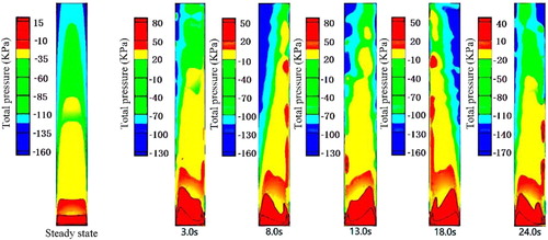
The total pressure distribution on the XOY surface of the conveyor pipeline at different time points is analyzed by examining the steady-state working condition and the swing amplitude of 1 m under the condition period of 20 s, and the result is presented in Figure 8. The time points are 3.0, 8.0, 13.0, 18.0, and 24.0 s. The figure demonstrates that the total pressure at the entrance of the conveyor pipeline considerably varies under the two working conditions, and the total pressure changes smoothly in the middle section of the pipeline. This phenomenon is mainly due to the relative slip between the solid–liquid two-phase control field and the solid phase at the entrance aggregation, resulting in a chaotic flow field and large energy loss.

The total pressure along the axial change is uniform under the steady-state condition, the total pressure distribution in the tube under the swing condition is chaotic, and the pressure value and distribution in the tube change with time. These findings indicate that the pipe swing has a substantial influence on the slurry conveying in the tube.

4.3.2. Effect of swing amplitude on pressure loss gradient

Figure 9 demonstrates that when the oscillation period is up to 20 s, the pressure loss gradient of the gas hydrate pipeline changes with time under different swing amplitude conditions. The swing amplitude includes six types of working conditions (0.5, 1.0, 3.0, 5.0, 8.0, and 10 m) to ensure full development of the fluid, and each working condition has a simulation time of 40 s.

Figure 9. Variation of pressure loss gradient of the conveying pipeline with time under different swing conditions. (a) Swing amplitude 0.5 m. (b) Swing amplitude 1.0 m. (c) Swing amplitude 3.0 m. (d) Swing amplitude 5.0 m. (e) Swing amplitude 8.0 m. (f) Swing amplitude 10 m.

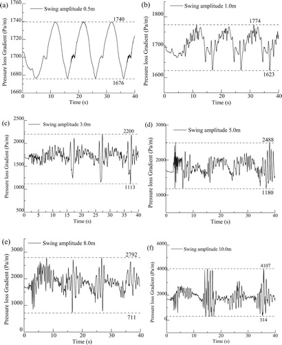
The figure also shows that the pressure loss gradient is periodic in the post-s period with a change cycle of 10 s, which is half of the pipeline oscillation cycle. When the oscillation amplitude is 0.25 m, the pressure loss gradient changes with the smooth curve with time, and the pressure loss gradient changes in the five remaining working conditions with the change in time. The pressure loss gradient changes are intense when the oscillation amplitude is large. The maximum values of the pressure loss gradient under the six operating conditions are 1740, 1774, 2200, 2488, 2792, and 4107 Pa/m. When the oscillation amplitudes are 0.25 and 0.5 m, the pressure loss gradient and steady-state condition are the same. Compared with the steady-state working conditions, the pressure loss gradient increases by 29.3% and 46.3% when the swing amplitudes are 1 and 2 m, respectively. When the swing amplitudes are 4 and 10 m, the pressure loss gradient respectively increases by 64.1% and 141.4% compared with that of the steady-state condition.

The variation amplitudes of pressure loss gradient under the six types of working conditions are 64, 151, 1087, 1308, 2081, and 3793 Pa/m. The change in pressure loss gradient becomes increasingly drastic with the increase in swing amplitude of the conveying pipeline.

When the swing amplitude is less than 0.5 m, the maximum and variation amplitudes of the pressure loss gradient are small. The maximum value and amplitude of the pressure loss gradient rapidly increase with the oscillation amplitude. When the swing amplitude exceeds 4 m, the pressure loss gradient of the conveying pipe dramatically changes, thus seriously affecting the stability of the conveying system.

The velocity changes during the pipeline oscillation process, and the collision between the solid-phase particles and the pipe wall increases under inertia. This phenomenon leads to the uneven distribution of solid particles in the flow field, resulting in pressure loss fluctuations of the conveying system. The phenomenon becomes evident when the oscillation is drastic. On the one hand, the system power design must choose the appropriate safety factor to ensure the normal operation of the conveyor system. On the other hand, the conveyor system swing must be minimized to improve the conveyor system stability. The aforementioned task is necessary to guarantee the normal operation of the conveyor system in the small swing.

4.4. Effect of lateral swing period on solid-phase average concentrations at the pipe outlet

The simulation analysis is conducted for six types of working conditions: the horizontal swing amplitudes are 1 and 2 m, and the swing periods are 10, 15, and 30 s. Figure 10 shows the variation of the average outlet concentration of the pipeline solid phase under the conditions of 10 s swing period and lateral swing amplitudes of 1 and 2 m. Figure 11 shows the variation of the average outlet concentration of the pipeline solid phase under the conditions of 15 s swing period and lateral swing amplitudes of 1 and 2 m. Figure 12 shows the variation of the average outlet concentration of the pipeline solid phase under the conditions of 30 s swing period and lateral swing amplitudes of 1 and 2 m.

Figure 10. Variation of the average outlet concentration of the pipeline solid phase under the condition of 10 s swing period and lateral swing amplitudes of 1 and 2 m. (a) Swing amplitude 1.0 m. (b) Swing amplitude 2.0 m.

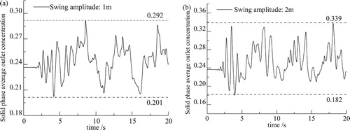
Figure 11. Variation of the average outlet concentration of the pipeline solid phase under the condition of 15 s swing period and lateral swing amplitudes of 1 and 2 m. (a) Swing amplitude 1.0 m. (b) Swing amplitude 2.0 m.

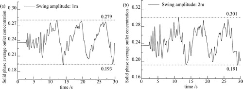
Figure 12. Variation of the average outlet concentration of the pipeline solid phase under the condition of 30 s swing period and lateral swing amplitudes of 1 and 2 m. (a) Swing amplitude 1.0 m. (b) Swing amplitude 2.0 m.

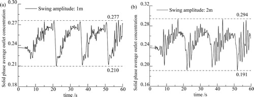
When the swing amplitude is 1 m, the maximum concentrations of the pipe outlet are 0.292, 0.279, and 0.277, and the concentration changes are 0.091, 0.086, and 0.067 under the conditions of 10, 15, and 30 s, respectively. The maximum outlet concentrations were 0.239, 0.301, and 0.294 when the swing was 2 m, and the concentration changes were 0.157, 0.11, and 0.103, respectively.

Figures 10–12 demonstrate that when the swing amplitude is the same, and the average value and the change amplitude of the solid-phase outlet slightly decrease with the increase in period. However, the change value is small. When the swing amplitude is constant, the speed change of the pipeline is aggravated by the shortening of the motion cycle. The collision of the solid-phase particles in the tube with the tube wall increases due to inertia. Accordingly, the slurry flow in the tube is disordered, and the outlet concentration of the pipeline is intensified. During the lateral swing of the pipe, the period of the solid-phase outlet concentration change is approximately 1/2 of the pipe oscillation period.

The swing amplitude increases from 1 to 2 m, and the amplitude of the solid-phase outlet concentration increases from 0.029–0.263. The oscillation period was reduced from 30 to 10 s, and the solid-phase outlet concentration variation amplitude increased from 0.067 and 0.103–0.091 and 0.157, respectively. The influence of the swing amplitude on the outlet concentration change amplitude is larger than the swing period. Therefore, controlling the variation range in the outlet concentration of the pipe by reducing the pipe swing amplitude is possible.

4.5. Influence of swing amplitude on the axial distribution of velocity in the Y-direction

The pipe oscillation period is set to 20 s, and the pipe oscillation amplitudes are A = 0.25, 0.5, 1.0, 2.0, 4.0, and 10.0 m. Figure 13 shows the distribution of the solid- and liquid-phase Y-direction velocities along the axial direction of the pipeline under the eight aforementioned conditions.

Figure 13. Two-phase velocity distribution in the conveying pipe under different swing conditions for a period of 20 s. (a) Y-direction solid-phase velocity. (b) Y-direction solid-phase velocity

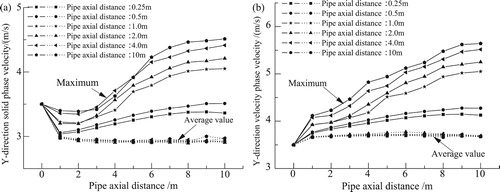
The solid and dotted lines in Figure 13 respectively represent the maximum value of each data and the average value of the corresponding parameters. Under different swing amplitudes, the maximum values of the solid–liquid and liquid-phase velocities in the pipeline are similar. The maximum velocity of the solid phase sharply decreases between 0 and 1 m after entering the pipeline, then 1–7. The distance between m slowly increases and finally reaches a relatively stable state between 7 and 10 m. After the liquid phase enters the pipeline, the maximum velocity rapidly increases from 0 to 1 m, gradually increases from 1 to 8 m, and then reaches a relatively stable state after 8 m. The maximum speed of the solid and liquid phases is large when the pipe swing amplitude is large.

The fluid inside the pipe is substantially affected by the force between gravity and solid–liquid two-phase control field immediately after entering the pipeline. Accordingly, the velocity considerably changes within 0–1 m. However, the difference between the maximum and the average speed of the solid and liquid phases is small at this stage. The influence of gravity and phase interaction stabilizes with the continuous transport of the fluid. The swing influence of the conveying pipe on the flow field emerges, as mainly manifested by the uneven distribution of the solid-phase particles in the tube. This phenomenon is attributed to the large and small slurry flow rates in the region with low and high solid-phase concentrations, respectively. The maximum speed of the conveying pipe is gradually increased from 1 to 7 m.

4. Experimental research

4.1. Experimental scenarios

The system parameters are selected on the basis of steady-state analysis to study the influence of pipeline movements on the solid–liquid two-phase flow field. Limited by the experimental conditions, the working conditions of this experiment mainly include the following: the influence of solid-phase concentration, particle size, and hydrate saturation on the pressure loss of the system under steady-state conditions. The change in system pressure loss when the transverse oscillation amplitudes of the pipeline are 0.25 and 0.5 m is investigated.

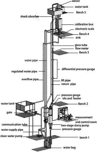
The experimental study must change the solid-phase concentration, particle size, and particle density (hydrate saturation) of slurry and test the pressure loss value under different working conditions. The solid-phase concentration is regulated by adjusting the speed control of the feeder, and the particle size and density are adjusted by using different models of simulated ore. The pressure loss is calculated by recording the pressure value of the working platform, and the pressure values of each group are recorded after the conveyor flow field reaches a stable state. The five data in each set of working conditions are recorded once at intervals of 1 min, and the average value is taken as the pressure loss values under this condition. Figure 14 shows the experimental system.

Figure 14. Structural schematic of the hydraulic transport system for deep-sea ore.

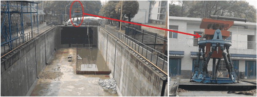
When simulating the lateral swaying experiment of the pipeline, the mining system is first suspended on the undulation experiment platform. Figure 15 demonstrates the structure of the undulation experimental platform, which made by the Changsha Research Institute of Mining And Metallurgy. The lifting pipe vibration law of the ore conveying system is jointly controlled by a wave experimental platform equipped with six hydraulic cylinders. The amplitude and vibration periods of the lifting pipe can be changed by setting different control parameters of the fluctuation experiment platform control program.

Figure 15. Simulation experiment platform of ore hydraulic conveying fluctuation.

In the transverse swing experiment of pipelines, the working parameters of the system remain unchanged, and the swing amplitude of the pipe is adjusted to 0.25 and 0.5. The oscillation period (20 s) has two types of working conditions. When the flow is stable, the maximum and minimum values of the pressure gauge within 5 min are recorded. The maximum and difference values of the pressure loss are calculated.

4.2. Analysis of experimental results

The pressure loss gradient of the conveying flow field under each working condition can be obtained by calculation and collating the experimental results. Tables 2–5 illustrate the comparison data between the experimental and the simulation results.

Table 2. Comparison of experimental and simulation results at different solid-phase concentrations.

	Pressure loss gradient /(Pa/m)
Solid-phase concentration	Experimental values	Simulation values	Deviation/%
0.1	1237.32	1173.97	5.12
0.15	1786.26	1665.90	6.74
0.2	2068.56	1990.94	3.75
0.25	2501.36	2367.46	5.35
0.3	2831.56	2707.57	4.56

Table 3. Comparison of experimental and simulation results under different particle sizes.

	Pressure loss gradient/(Pa/m)
Granular particle size/mm	Experimental values	Simulation values	Deviation/%
10	1896.32	1844.17	2.75
20	2068.56	1990.94	3.75
30	2213.63	2082.16	5.94
40	2296.35	2126.76	7.39

Table 4. Comparison of experimental and simulation results of hydrate under different saturations.

	Pressure loss gradient/(Pa/m)
Hydrate saturation/%	Experimental values	Simulation values	Deviation/%
10	2613.25	2498.45	4.39
20	2359.65	2215.39	6.11
30	2068.56	1990.94	3.75
40	1863.25	1775.09	4.73
50	1508.32	1401.83	7.06

Table 5. Comparison of experimental and simulation results under different swing conditions of the pipeline.

	Maximum value/(Pa/m)			Variation amplitude/(Pa/m)
Swing amplitude/m	Experimental values	Simulation values	Deviation/%	Experimental values	Simulation values	Deviation/%
0.5	2096.32	2037.73	2.79	109.12	102.69	5.89
1	2135.56	2076.35	2.77	215.36	206.25	4.23

As shown in the data comparison presented in the table, the numerical and experimental results are similar, and the deviation between the two is within 7.39%. The experimental results are slightly larger than the numerical results. The above comparison demonstrates the credibility of the numerical simulation results in the present work. The numerical and experimental results are analyzed, and the deviation is due to the following reasons.

1. The numerical mode calculation using the conveyor pipe wall is smooth, and the pipeline is assembled. The pipe road is equipped with a flow meter, a pressure gauge, and other instruments. The transport process will produce local pressure loss.

2. The numerical calculation assumes that the solid-phase particles are regular spherical, and the shape of the solid-phase particles in the experiment exhibits deviation. Some particles will appear broken after the pump, demonstrating an irregular shape.

5. Conclusion

A numerical simulation model of the solid–liquid two-phase flow field in a conveyor pipeline is established on the basis of the study of computational fluid mechanics. The aforementioned flow field is numerically simulated by CFD simulation software. The influence law of pipeline swing on the solid-phase average concentration, solid-phase distribution, pressure distribution, and pressure loss of the pipeline outlet is obtained under the ocean dynamic environment. Finally, the reliability and accuracy of the simulation results are verified by experiments. The main conclusions are as follows.

1. The dynamic grid model of CFD is used to simulate the pipeline movement in a marine dynamic environment. The research shows that the disturbance of the transverse swing convection field of pipelines is large, and the influence of the axial vibration convection field is small. Under the lateral swinging condition of the pipeline, the pressure loss gradient periodically changes with time, and the change period is half of the pipeline movement period. The maximum value and variation amplitude of the pressure loss gradient increase with the pipe oscillation amplitude and decrease with the increase in the oscillation period.

2. The influence of different oscillation amplitudes and periods of conveying pipelines on the conveying flow field is analyzed. The results show that the flow field and steady-state condition of the conveying pipeline are the same when the transverse oscillation amplitude does not exceed 0.5 m. After the swing amplitude exceeds 1 m, the oscillation has a considerable influence on the solid-phase distribution of the conveyor flow field, solid–liquid two-phase velocity, dynamic and static pressure, and pressure loss. The flow field distribution is chaotic when the transverse oscillation period of the pipeline is small. This phenomenon is highly evident with large oscillation amplitude.

3. The phase change of natural gas hydrates during transportation is a continuous process. This phenomenon results in a more complicated natural gas hydrate hydraulic conveying process than other hydraulic or pneumatic conveying processes. The current CFD simulation software has no model that can be used directly for the continuous simulation of the process. Subsequent studies can consider the preparation of the hydrate decomposition model by the UDF module in CFD software based on phase transition theory of natural gas hydrates. Moreover, the continuous numerical calculation of the solid–liquid two-phase flow and the solid–liquid three-phase flow can be realized in the hydrate transport process.

Acknowledgements

This work was supported by the National Natural Science Foundation of China (51775561); Natural Science fund of Hunan Province (2018JJ2522); Science and Technology Plan Project of Loudi City (2018KJJ005).

Disclosure statement

No potential conflict of interest was reported by the author(s).

Additional information

Funding

This work was supported by the National Natural Science Foundation of China (51775561); Natural Science foundation of Hunan Province (2018JJ2522); Science and Technology Innovation Project of Loudi City (2018KJJ005).

References

- Camenen, B. (2007). Simple and general formula for the settling velocity of particles. Journal of Hydraulic Engineering, 133(2), 229–233. doi: 10.1061/(ASCE)0733-9429(2007)133:2(229)
- Chung, J. S. (1998). An articulated pipe-miner system with thrust control for deep-ocean crust mining. Marine Georesources & Geotechnology, 16(4), 253–271. doi: 10.1080/10641199809379971
- Eivaz, A., Bahman, N., Mohsen, J., Sina, F. A., Shahaboddin, S., & Kwok-Wing, C. (2018). Experimental and computational fluid dynamics-based numerical simulation of using natural gas in a dual-fueled diesel engine. Engineering Applications of Computational Fluid Mechanics, 12(1), 517–534. doi: 10.1080/19942060.2018.1472670
- Felippa, C. A., & Chung, J. S. (1981). Nonlinear static analysis of deep ocean mining pipe-part I: Modeling and formulation. Journal of Energy Resources Technology, 103(1), 11–15. doi: 10.1115/1.3230807
- Ghalandari, M., Mirzadeh Koohshahi, E., Mohamadian, F., Shamshirband, S., & Chau, K. W. (2019). Numerical simulation of nanofluid flow inside a root canal. Engineering Applications of Computational Fluid Mechanics, 13(1), 254–264. doi: 10.1080/19942060.2019.1578696
- Ihle, C. F. (2013). A cost perspective for long distance ore pipeline water and energy utilization. Part I: Optimal base values. International Journal of Mineral Processing, 122, 1–12. doi: 10.1016/j.minpro.2013.04.002
- Li, L., Xu, H. L., & Yang, F. Q. (2015). Three-phase flow of submarine gas hydrate pipe transport. Journal of Central South University, 22(9), 3650–3656. doi: 10.1007/s11771-015-2906-y
- Liu, S. J., Hu, J. H., & Dai, Y. (2017). Flow field analysis and parameter optimization of deep-sea polymetallic sulphide aggregate shousing. Journal of Central South University (Natural Science Edition), 48(5), 1198–1203.
- Makogon, Y. F. (2010). Natural gas hydrates: A promising source of energy. Journal of Natural Gas Science and Engineering, 2(1), 49–59. doi: 10.1016/j.jngse.2009.12.004
- Mohebbi, V., & Behbahani, R. M. (2014). Experimental study on gas hydrate formation from natural gas mixture. Journal of Natural Gas Science and Engineering, 18, 47–52. doi: 10.1016/j.jngse.2014.01.016
- Mosavi, A., Shamshirband, S., Salwana, E., Chau, K. W., & Tah, J. H. M. (2019). Prediction of multi-inputs bubble column reactor using a novel hybrid model of computational fluid dynamics and machine learning. Engineering Applications of Computational Fluid Mechanics, 13(1), 482–492. doi: 10.1080/19942060.2019.1613448
- Mou, B., He, B. J., Zhao, D. X., & Chau, K. W. (2017). Numerical simulation of the effects of building dimensional variation on wind pressure distribution. Engineering Applications of Computational Fluid Mechanics, 11(1), 293–309. doi: 10.1080/19942060.2017.1281845
- Osorio, A. F., Ortega, S., & Arango-Aramburo, S. (2015). Assessment of the marine power potential in Colombia. Renewable and Sustainable Energy Reviews, 56, 966–977.
- Payne, G. S., Kiprakis, A. E., Ehsan, M., Rampen, W. H. S., & Wallace, A. R. (2007). Efficiency and dynamic performance of digital displacement (tm) hydraulic transmission in tidal current energy converters. Proceedings of the Institution of Mechanical Engineers, Part A: Journal of Power and Energy, 221(2), 207–218.
- Pei, J., Wang, W. J., & Yuan, S. Q. (2014). Statistical analysis of pressure fluctuations during unsteady flow for low-specific-speed centrifugal pumps. Journal of Central South University, 21(3), 1017–1024. doi: 10.1007/s11771-014-2032-2
- Rajnauth, J., & Barrufet, M. (2012). Monetizing gas: Focusing on developments in gas hydrate as a mode of transportation. Energy Science and Technology, 4(2), 61–68.
- Ramezanizadeh, M., Alhuyi Nazari, M., Ahmadi, M. H., & Chau, K. W. (2019). Experimental and numerical analysis of a nanofluidic thermosyphon heat exchanger. Engineering Applications of Computational Fluid Mechanics, 13(1), 40–47. doi: 10.1080/19942060.2018.1518272
- Song, W. J., Xiao, R., & Feng, Z. P. (2010). Solid-liquid two-phase flow simulation on particle deposition velocity using for latent heat transportation. Journal of Engineering Thermophysics, 31(10), 1693–1696.
- Van Wijk, J. M., Talmon, A. M., & Van Rhee, C. (2016). Stability of vertical hydraulic transport processes for deep ocean mining: An experimental study. Ocean Engineering, 125, 203–213. doi: 10.1016/j.oceaneng.2016.08.018
- Wang, Z. J. (2016). A perspective on high-order methods in computational fluid dynamics. Science China (Physics. Mechanics & Astronomy), 59(01), 7–12.
- Wang, L., Liu, Z. Y., Abdelkefi, A., Wang, Y. K., & Dai, H. L. (2017). Nonlinear dynamics of cantilevered pipes conveying fluid: Towards a further understanding of the effect of loose constraints. International Journal of Non-Linear Mechanics, 95, 19–29. doi: 10.1016/j.ijnonlinmec.2017.05.012
- Wu, B., Wang, X. L., Liu, H., & Xu, H. L. (2015). Numerical simulation and analysis of solid-liquid two-phase three-dimensional unsteady flow in centrifugal slurry pump. Journal of Central South University, 22(8), 3008–3016. doi: 10.1007/s11771-015-2837-7
- Xu, H. L., Chen, W., Wu, B., & Yang, F. Q. (2016). Characteristic of cutting head in marine gas hydrate by cutter suction exploitation. Sichuan Daxue Xuebao (Gongcheng Kexue Ban)/Journal of Sichuan University (Engineering Science Edition), 48(6), 126–131.
- Yuliang, Z., Yi, L. I., Baoling, C., Zuchao, Z., & Huashu, D. (2013). Numerical simulation and analysis of solid-liquid two-phase flow in centrifugal pump. Chinese Journal of Mechanical Engineering, 01, 57–64.
- Zou WS, & Huang JY. (2006). Ocean mining technology for deep-sea mining of manganese nodules. Mining and Metallurgy Engineering, 25(3), 1–5.