Study on hydrodynamics of a flexible fishlike foil undulating in wall effect

Abstract

This paper aims to investigate the hydrodynamics of a flexible fishlike foil undulating near the vertical sidewall by using numerical simulation. To achieve the research target of this paper, an immersed boundary-lattice Boltzmann method (IB-LBM) was proposed for high Reynolds number fluid flow simulation. The influences of the clearance (0.2L ≤ d ≤ 0.8L, L is the chord length of the fishlike foil) between the fishlike foil and sidewall, Strouhal number (0.1 ≤ St ≤ 0.5), and wavelength (0.6L ≤ λ ≤ 1.4L) on the hydrodynamic characteristics and power extraction efficiency were studied. The results indicate that the wall effect on forces increase with increasing St and λ, but it is opposite for the power extraction efficiency. As compared to the case of out of wall effect, the fishlike foil swims near the sidewall has an effect of improving thrust and it will reduce or increase the power extraction efficiency in some specified cases. Moreover, an interesting phenomenon with pair arrayed vortices, pair arrayed low-pressure centers and pair arrayed high-velocity centers are observed due to the presence of sidewall.

KEYWORDS:

• Wall effect
• flexible fishlike foil
• hydrodynamics
• power extraction efficiency

1. Introduction

Inspired by the astonishing swimming abilities of fish, various Autonomous Underwater Vehicles (AUVs) were developed by humans. Fish with body/caudal fin (BCF) propulsion mode has the merit of high efficiency and high maneuverability, and it has been a focus for biomimetic propulsion systems (Roper et al., 2011). Various experiments and simulations have been conducted by previous researchers to reveal the BCF swimming mechanism of fish (Lighthill, 1969; M. S. Triantafyllou, Triantafyllou, & Yue, 2000; Borazjani & Sotiropoulos, 2008; Scaradozzi et al., 2017). It was found that during swimming, the vortices generated by the caudal fin of fish have the benefit for energy conservation. The dimensionless parameters of Reynolds number (Re) and Strouhal number (St) have significant effects on the hydrodynamics performance of fish. However, the underwater environment is complex. Various external disturbances will affect the swimming performance of the fish. Study on the interaction between fish swimming and flow environment is meaningful for achieving efficient designs of bionic AUV.

Live fish are often swimming near the ground to predation (Blevins & Lauder, 2012), and a large number of practical engineering applications also require bionic AUV to propel steadily near the ground for various underwater operations. Fish swims near a solid boundary show different hydrodynamic features, which commonly called ‘ground effect’ (Clark & Smits, 2006). Besides, ground effect also widely appeared in birds and insects near ground fighting (Wu et al., 2014; Gao & Lu, 2008; Truong et al., 2013; Wu et al., 2015) and aircraft taking off and landing (Moryossef & Levy, 2004; Molina & Zhang, 2011). The previous studies concerning about the ground effect can be divided into two types, steady ground effect and unsteady ground effects. The steady ground effect has been widely studied (Rozhdestvensky, 2006), and it commonly considered for rigid and static structures, such as fixed-wing airfoils (Coulliette & Plotkin, 1996). In contrast, the unsteady ground effects appeared in the situation of flyers and swimmers oscillate their wings or fins near to a solid ground have not been widely studied. Tanida (2001) studies a fluttering plate in a wind tunnel by using the linearized Euler equations, which is the earliest analytical approach to investigate the ground effect. Most numerical (Srinidhi & Vengadesan, 2017; Moryossef & Levy, 2004) and experimental (Quinn, Moored, et al., 2014; Mivehchi et al., 2016) works on unsteady ground effect are almost concerning rigid flapping wings/fins only. However, in the case of fish, the situation of such a flexible undulating body moving near to the boundary is significantly different from the rigid flapping wings/fins mentioned above. It is relevant both to a fish (like trout and bluegill sunfish) with a very narrow ventral span swimming near a vertical wall and to a flatfish (like European plaice) swimming near the bottom ground. Blevins and Lauder (2013) proposed a simplified physical model based on the freshwater stingray and the effects of a solid ground on undulating movement was examined. (Quinn, Lauder, et al., 2014) present experimental evidence for the hydrodynamic benefits of dorsoventrally compressed form swimming, which demonstrates that fish swimming near the ground can produce more thrust and improve propulsive efficiency. In nature, most fish are laterally compressed and swim ‘upright’ (Webb, 2002). When swimming close to a vertical sidewall, the wall effect starts to work. However, seldom works can be found for such a swimming form and the wall effect experienced by the flexible undulating fish body is unknown.

In this paper, we employ a flexible fishlike foil with BCF propulsion mode resembling the carangiform swimming and conduct a systematic study on the hydrodynamics performance of the fishlike foil undulating in the wall effect by using of immersed boundary-lattice Boltzmann method (IB-LBM). Parameters like the swimming frequency, body wavelength, and clearance between fishlike foil and sidewall were systematically studied to reveal the characteristics of the wall effect. It is essential to investigate the wall effect on the fish swimming, which will promote the application of bionic AUV.

2. Problem description and methodology

2.1. Problem description

In this study, a 2D fishlike foil is used to model the flexible fish body in the forward-swimming mode near a vertical sidewall. As shown in Figure 1, L is the foil chord length, and d is the clearance between the centerline of the foil and sidewall. In the natural environment, there are two wall situations to be modeled: (a) a fish swimming in a stream (like river trout), (b) a fish swimming in a calm lake or sea (like European plaice), or an aquarium. A boundary layer near the wall should be modeled in case (a) (Quinn, Moored, et al., 2014), while in the case (b), it should avoid having a boundary layer since it is absent in stagnant calm water. Here, we focused on the case (a), and a no-slip boundary condition is applied at the sidewall and foil edges. U indicates the constant incoming flow velocity. Here, the dimensionless parameter Reynolds number is expressed as $R_e=\rho UL/\phantom{\rho UL\mu }\mu$. ρ indicates the fluid density, and µ indicates the fluid dynamic viscosity. Considering the real fish swimming, fish has higher propulsion efficiency at large Reynolds number (Barrett et al., 1999). Therefore, in this study, the Re is set as 8 × 10⁴.

Figure 1. Schematics of the computational model.

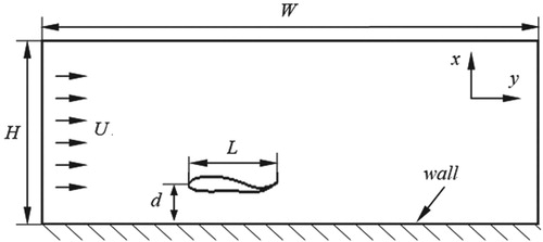
We treat the fishlike undulating foil as a carangiform swimmer whose motion can be can be given by Videler and Hess (1984), (1) $\begin{array}{rl}y(x,t)& =A\left(x\right)\sin (kx-2\pi ft)\end{array}$(1) (2) $\begin{array}{rl}A\left(x\right)& =a_0+a_{1}x+a_2{x}^2\end{array}$(2) where x is measured from the tip of the fish head; A(x) is the amplitude envelope of lateral motion with the coefficients a₀ = 0.02, a₁ = −0.008 and a₂ = 0.16 to ensure the maximum displacement at the fishtail (Liu & Kawachi, 1999); y(x,t) is the lateral excursion at time t; k = 2π/λ is the wavenumber, λ indicates the wavelength; f and t are the frequency and time respectively.

2.2. Numerical method

In this study, a robust immersed boundary-lattice Boltzmann method (IB-LMB) was employed to determine the wall effect when the fishlike foil swimming near the sidewall. The lattice Boltzmann method (LBM) was initially proposed by McNamara and Zanetti (1988). Here, considering the high Reynolds number fluid flow applications, a kind of LBM combined with LES models (Hou et al., 1996) is employed. Besides, for fluid-structure interaction of moving objects, some new methods have been developed to deal with the complex dynamic mesh problems (Salih et al., 2019; Ghalandari et al., 2019). The immersed boundary method (IBM) (Mittal & Iaccarino, 2005) as a boundary treatment method has evolved into an effective way for fluid-structure interaction applications, and it was employed to resolve the dynamic boundary problems of the undulating foil in this study. In this method, the flow field Ω was solved on a Cartesian grid x, and the boundary of the foil Γ was imitated by a series of Lagrangian points X(s,t) (0 < s < L_b) loaded with external forces.

The D2Q9 model is employed in this study, and the filtered governing equations (Hou et al., 1996; Guo et al., 2002) of the IB-LBM framework can be written as (3) $\begin{array}{rl}& {\overline{f}}_{\alpha }(x+e_{\alpha }\delta t,t+\delta t)-{\overline{f}}_{\alpha }(x,t)\\ & =-\frac{1}{{\tau }_{\text{total}}}\left[{\overline{f}}_{\alpha }\right(x,t)-{\overline{f}}_{\alpha }^{eq}(x,t\left)\right]+g_{\alpha }(x,t)\delta t\end{array}$(3) (4) $\begin{array}{rl}{\overline{f}}_{\alpha }^{eq}(\mathit{x},t)& =\overline{\rho }{\omega }_{\alpha }\left[1+\frac{{\mathit{e}}_{\alpha }\cdot \overline{\mathit{u}}}{c_s^2}+\frac{{({\mathit{e}}_{\alpha }\cdot \overline{\mathit{u}})}^2}{2c_s^4}-\frac{\overline{\mathit{u}}\cdot \overline{\mathit{u}}}{2c_s^2}\right]\end{array}$(4) (5) $\begin{array}{rl}{g}_{\alpha }(\mathit{x},t)& =\left(1-\frac{1}{2\tau }\right){\omega }_{\alpha }\left[\frac{{\mathit{e}}_{\alpha }-\mathit{u}}{c_s^2}+\frac{{\mathit{e}}_{\alpha }\cdot \mathit{u}}{c_s^4}{\mathit{e}}_{\alpha }\right]\cdot \mathit{f}\end{array}$(5) (6) $\begin{array}{rl}\rho \mathit{u}& =\sum _{\alpha }{\mathit{e}}_{\alpha }{f}_{\alpha }+\frac{1}{2}\mathit{f}\delta t\end{array}$(6) where ${\overline{f}}_{\alpha }$ is the filtered distribution function for particles with velocity e_α; ${{\overline{f}}_{\alpha }}^{eq}$ is the equilibrium distribution function; τ_total is the relaxation time; δ_t is the time increment; ω_α represents the coefficients related to the lattice velocity used in the model; c_s is the speed of sound in the lattice model, and f is the force density at the Eulerian point.

The relaxation time, τ_total, be a function of total viscosity v_total as show (7) $\frac{2{\tau }_{\text{total}}-1}{6}=v_{\text{total}}$(7)

Based on the Smagorinsky model (Smagorinsky, 1963), the total viscosity equals the sum of the physical and eddy viscosities, and the τ_total can be obtained by (8) ${\tau }_{\text{total}}=3v_{\text{total}}+\frac{1}{2}=3(v_0+C{\mathrm{\Delta }}^2|\overline{S}|)+\frac{1}{2}$(8) where $C{\mathrm{\Delta }}^2|\overline{S}|$ indicates the eddy-viscosity term and v₀ indicates the physical kinematic viscosity.

The velocity at all boundaries is set to be equal to the velocity of the fluid at the same location to satisfy the no-slip boundary condition (Wu et al., 2015): (9) $\mathit{A}\mathit{X}=\mathit{B}$(9) where $\begin{array}{rl}X& =\{\delta u_B^1,\delta u_B^2,\dots ,\delta u_B^m{\}}^m\end{array}$ $\begin{array}{rl}\mathit{A}& =\left(\begin{array}{cccc}{\delta }_{11}& {\delta }_{12}& \cdots & {\delta }_{1n}\\ {\delta }_{21}& {\delta }_{22}& \cdots & {\delta }_{2n}\\ ⋮& ⋮& \ddots & ⋮\\ {\delta }_{m1}& {\delta }_{m2}& \cdots & {\delta }_{mn}\end{array}\right)\\ & \times \left(\begin{array}{cccc}{\delta }_{11}^B& {\delta }_{12}^B& \cdots & {\delta }_{1m}^B\\ {\delta }_{21}^B& {\delta }_{22}^B& \cdots & {\delta }_{2m}^B\\ ⋮& ⋮& & ⋮\\ {\delta }_{n1}^B& {\delta }_{n2}^B& \cdots & {\delta }_{nm}^B\end{array}\right)\end{array}$ $\mathit{B}=\left(\begin{array}{c}{U}_B^1\\ U_B^2\\ ⋮\\ U_B^m\end{array}\right)-\left(\begin{array}{cccc}{\delta }_{11}& {\delta }_{12}& \cdots & {\delta }_{1n}\\ {\delta }_{21}& {\delta }_{22}& \cdots & {\delta }_{2n}\\ ⋮& ⋮& \ddots & ⋮\\ {\delta }_{m1}& {\delta }_{m2}& \cdots & {\delta }_{mn}\end{array}\right)\left(\begin{array}{c}{u}_1^{\ast }\\ u_2^{\ast }\\ ⋮\\ u_n^{\ast }\end{array}\right)$where m is the Lagrangian points number, and n is the surrounding Eulerian mesh points number; $U_B^l$ is the boundary velocity; $\delta {\mathbf{u}}_B^l(l=1,2,\dots ,m)$ is the unknown velocity correction vector of the boundary points;${\delta }_{ij}^{}=D_{ij}({\mathbf{x}}_{ij}-{\mathbf{X}}_B^l)\mathrm{\Delta }x\mathrm{\Delta }y$, ${\delta }_{ij}^B=D_{ij}({\mathbf{x}}_{ij}-{\mathbf{X}}_B^l)\mathrm{\Delta }{s}_l$. $\mathrm{\Delta }{s}_l$ is the arc length of the boundary element, and $D_{ij}({\mathbf{x}}_{ij}-{\mathbf{X}}_B^l)$ is a smooth 2-point piecewise delta function proposed by Peskin (2002) which can be written as (10) $D_{ij}({\mathbf{x}}_{ij}-{\mathbf{X}}_B^l)\text{ = }\frac{1}{h^2}{\delta }_h\left(\frac{x_{ij}-X_B^l}{h}\right){\delta }_h\left(\frac{y_{ij}-Y_B^l}{h}\right)$(10) ${\delta }_h\left(r\right)=\left\{\begin{array}{l}\frac{1}{4}\left[1+\cos \left(\frac{\pi r}{2}\right)\right],|r|\le 2\\ 0,,|r|\ge 2\end{array}\right.$where h is the mesh spacing. Moreover, the intermediate fluid velocity ${\mathit{u}}^{\ast }$ can be obtained by (11) ${\mathit{u}}^{\ast }=\frac{1}{\rho }\sum _{\alpha }{e}_{\alpha }{f}_{\alpha }$(11)

Besides, we can obtain the unknown $\delta u_B^l$ by solving the Equation (9). Then, the fluid velocity correction$\delta \mathit{u}$ is given by (12) $\delta \mathit{u}\left(x_{ij}\right)=\sum _l\delta u_B^l\left(X_B^l\right)D_{ij}(x_{ij}-X_B^l)\mathrm{\Delta }{s}_l$(12)

According to the Equation (6), the force density f as a function of the $\delta \mathit{u}$ can be represented as $\mathit{f}=2\rho \delta \mathit{u}/\delta t$. Correspondingly, the force on the boundary point is obtained by (13) $F\left(X_B^l\right)=\frac{2\rho \delta {\mathit{u}}_B^l\left(X_B^l\right)}{\delta t}$(13)

Besides, other macroscopic variables of mass density ρ and pressure P are calculated by the distribution functions. (14) $\rho \text{ = }\sum _{\alpha }{f}_{\alpha },P=c_s^2\rho$(14)

2.3. Numerical validation

To validate the present code and methods, the published experimental data reported by Anderson et al., (1998) was employed. An experimental apparatus with a NACA0012 foil was developed by Anderson, and a series of experiments were conducted under various conditions of oscillation. 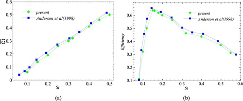Here, a NACA0012 rigid foil simulation model is established, as shown in Figure 2, and we chose the oscillating parameters of heave amplitude-to-chord ratio h_o/c = 0.25, phase angle $\psi$ = 90° and maximum angle of attack ${\alpha }_{max}$ = 15° for comparison. The average thrust coefficient and propulsion efficiency in this paper are defined consistent with the work of Anderson. As shown in Figure 3, the average thrust coefficient and propulsion efficiency calculated by using of the present numerical method are quite similar to the experimental data proposed by Anderson. Thus, the computational method adopted in this paper meets our requirement and credible.

Figure 2. NACA0012 foil simulation model.

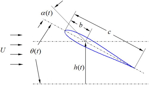
Figure 3. Comparison of the present result and previous data for the (a) average thrust coefficient $\overline{Ct}$ and (b) propulsion efficiency.

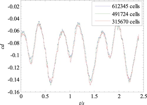
To validate the accuracy of our data in the current study, three grid systems with different cell numbers (rough grid with 315,670 cells, medium grid with 491,724 cells, and fine grid with 612,345 cells) were employed, and the simulation parameters were chosen as d = 0.2L, St = 0.25. Figure 4 shows the time-varying cd curves under different grids systems. It is obvious that the calculation results are identical in the three cases. The larger grids number has benefits for flow field structure but costs more computing time as well. Therefore, the medium mesh is employed for this calculation.

Figure 4. The time-varying drag coefficient curves over three cycle using different grids.

2.4. Hydrodynamics parameters

When fishlike foil undulating near the sidewall, the mean lift $\overline{Cl}$, moment $\overline{Cm}$ and thrust coefficients $\overline{Ct}$ are defined as (15) $\begin{array}{r}\overline{Cl}=\frac{{\int }_0^T{F}_l\left(t\right)dt}{0.5T\rho L{U}^2},\overline{Cm}=\frac{{\int }_0^{T}M\left(t\right)dt}{0.5T\rho L{U}^2},\overline{Ct}=\frac{{\int }_0^T{F}_T\left(t\right)dt}{0.5T\rho L{U}^2}\end{array}$(15) where F_l(t), M(t) and F_T(t) represent the instantaneous lift, moment and thrust force, respectively; T indicates the motion cycle; U indicates the constant incoming flow velocity and ρ indicates the fluid density. The moment center is set in L/2 of the foil.

In addition, the fishlike foil undulating in moving fluid, the thrust forces are mainly composed of friction thrust F_f and pressure difference thrust F_p. Thus, the power for lateral oscillation of the fishlike foil is expressed as (Ji & Huang, 2017): (16) $P_s={\oint }_S(F_f+F_p)v_{y}ds$(16) where v_y is the y-direction component of the fishlike foil surface velocity, S demonstrates the foil body curve and ds demonstrates the infinitesimal element of the curve.

The total energy consumption is expressed as (17) $E=\frac{1}{2}m{U}^2=\frac{1}{2}\left(\rho AU\right)U^2$(17) where A is the maximum lateral excursion of foil over an undulating cycle. Therefore, the power extraction efficiency can be written as (18) $\eta =\frac{P_s}{E}$(18)

3. Results and discussions

In order to reveal the wall effect at different Strouhal number $St=fA/\phantom{fAU}U$ and wavelength λ, six groups of parameters are selected for each variable in our work, as shown in Table 1. St was employed to indicate the effect of foil undulating frequency on swimming performance. U is supposed to be 0.8m/s, and A is set as 0.2L. Therefore, St represents the variation of undulating frequency. The force and power extraction efficiency are calculated at various St and λ. In order to further study the mechanisms of the wall effect, the details of flow field structure around the fishlike foil are considered, especially the vortex structure in the wake.

Table 1. Simulation parameters arrangement (d = ∞ denotes out of wall effect case).

d	St	λ
0.2L, 0.3L, 0.4L, 0.6L, 0.8L, ∞	0.1, 0.2, 0.25, 0.32, 0.4, 0.5	0.6L, 0.8L, 1.0L, 1.2L, 1.4L

3.1. Effect of Strouhal number

For given λ = 1.0L, the mean thrust $\overline{Ct}$, lift $\overline{Cl}$ and moment $\overline{Cm}$ coefficients, and power extraction efficiency η against Strouhal number St at different clearance d are plotted in Figure 5. As a reference, the results of out of wall effect case (denoted as d = ∞) are also plotted in these figures. To mimic the case of out of wall effect, the fishlike foil is initially located at d = 10L.

Figure 5. The mean (a) thrust $\overline{Ct}$, (b) lift $\overline{Cl}$, (c) moment $\overline{Cm}$ coefficients and (d) power extraction efficiency η against Strouhal numbers St at different clearance d.

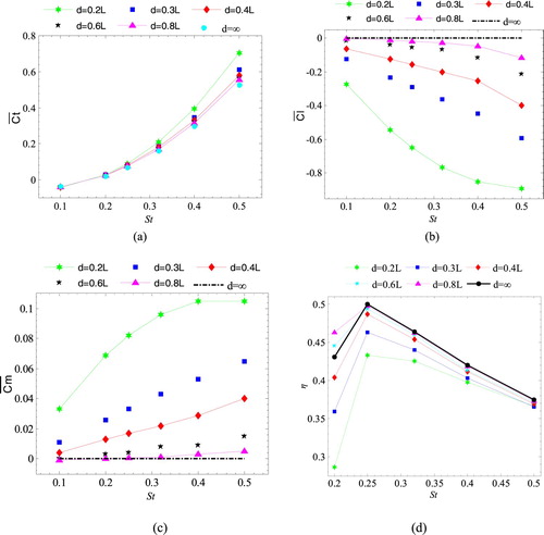
As shown in Figure 5(a), the mean thrust coefficient $\overline{Ct}$ is increases monotonically with St for all cases. This trend meets to the experimental result given by Anderson et al. (1998). The data dispersion of $\overline{Ct}$ at different d gradually increased with increasing of St. For a given St, smaller the d, larger is $\overline{Ct}$. Those trends indicate that the wall effect on $\overline{Ct}$ increase with increasing of St and near sidewall swimming has an effect of improving thrust. This phenomenon can also be found on the aerofoil undergoing pitch oscillations in ground effect (Quinn, Lauder, et al., 2014) and the flexible rectangular panels(mimic dorsoventrally compressed form fish) undulating near the ground (Quinn, Lauder, et al., 2014; Fernández-Prats et al., 2015).

As shown in Figure 5(b,c), the $\overline{Cl}$ and $\overline{Cm}$ have similar variation trend with $\overline{Ct}$. Since the fishlike foil undulates symmetrically, it is easy to assume that $\overline{Cl}$ and $\overline{Cm}$ are zero (as shown by the black dotted line) for the case of out of wall effect. However, in this study, it is evident to note that $\overline{Cl}$ is negative in all cases, which demonstrates that the foil suffers a lift force pointing to the sidewall. Furthermore, when undulating near the sidewall, the foil generates a positive torque which leads to a yaw motion closed to the sidewall. Compared with $\overline{Ct}$ curves, the data dispersion of $\overline{Cl}$ and $\overline{Cm}$ at different d is more significant, which indicate that the wall effect has more considerable influence on $\overline{Cl}$ and $\overline{Cm}$ than that on $\overline{Ct}$. Here, two relevant situations should be discussed: (a) a laterally compressed fish (like trout) swimming near a vertical sidewall; (b) a flatfish (like European plaice) swimming near the bottom ground. European plaice (and similar species) developed asymmetrical form (flat lower part and convex upper part). Such a structure is only convenient for lying at the bottom ground, but it is also suitable for swimming since the asymmetric structure prevents the problem with force directed toward the bottom ground. By detailed observation of the swimming style developed by European plaice (and similar flatfish), we can noticed that the central part of the body undergoes relatively small undulations (and thereby serves as a wing to fix the problems with the near-bottom lift force) while the periphery of the body is performing an undulatory motion (often with relatively small wavelength) thereby providing thrust. In contrast, trout (and similar species) experience slight ground effects when swimming close to the bottom ground. Still, they can experience considerable wall effect when undulating near the vertical sidewall. How to adjust the lift force to keep fish swimming at a fixed distance from the sidewall is still an unknown problem.

Figure 5(d) shows the curves of power extraction efficiency η against St at different d, as can be seen, the η initially increases with increasing St, and a peak value appeared at St = 0.25, then decreases with further increasing of St. The variation trend of power extraction efficiency meet the experimental test conducted by Anderson et al. (1998). Furthermore, Rohr et al. (1998) proposed that the St of swimming dolphins is around 0.25 for numerous observations of trained dolphins, showing good agreement with present simulation. Also of interest is that this is a rather general observation emphasized by Gazzola et al., (2014), who demonstrate that for Re > 10,000, the St for a large variety of fish is around 0.3. Same is often true for flapping rigid foils: (Triantafyllou et al., 1993) found that the optimum St for a number of specific profiles is between 0.25 and 0.35. Moreover, within the computational range, the maximum efficiency is 49.7% at d = 0.8L, St = 0.25, and the minimum efficiency appeared at d = 0.2L, St = 0.2 with the value η = 26.6%. Compared to the out of wall effect case (d = ∞), η is higher at d = 0.6L and d = 0.8L for St ≤ 0.25, which indicate that wall effect can improve power extraction efficiency in some cases and also reduce efficiency in other specific case. This result neither agrees with the view that power requirements increase when fish swimming near the ground (Blevins & Lauder, 2013)nor meets the points that the fish swimming efficiency improved due to the presence of ground (Quinn, Moored, et al., 2014; Fernández-Prats et al., 2015). In addition, the data dispersion of η at different d decreased gradually with increasing of St, which demonstrate that the influence of wall effect on η decrease with increasing St.

 Figure 6 exhibits the instantaneous vorticity contours at d = 0.2L under different Strouhal number St. For comparison, the vorticity distribution at d = 10L is employed to mimic the case of out of wall effect. In these figures, the red and blue indicate the vorticity with counterclockwise and clockwise (CW) direction, respectively. A regular reverse Karman Street appeared in the weak when the fishlike foil oscillates without wall effect (see Figure 6(b)). In comparison, the vortices have significant interaction with the sidewall when the foil is undulating near the sidewall. As can be seen in Figure 6(a), the vortex length changed into short extremely at low St(=0.1 and 0.2) due to the wall effect. With increasing of St (=0.25, 0.35 and 0.4), the strength of vortices becomes stronger, and the vortices arrayed in pairs in the wake due to the presence of the sidewall. Similar pairing vortices are also observed in the experiment of rigid pitching aerofoil propelled to near the ground proposed by Quinn, Moored, et al., (2014), Moored et al., (2014). Furthermore, it is obvious to find that the vortices move gradually far away from the sidewall and the angle between the sidewall and the centerline of the vortex street increase with increasing St and this phenomenon has also been reported by Wu et al. (2014) in the study of insect wing flapping near the ground.

Figure 6. Instantaneous vorticity contours against Strouhal number St at (a) d = 0.2L and (b) d = 10L.

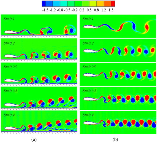
According to the theory of vortex dynamics (Zhu & Yu, 2017), the relationship between the strength of the vortex and thrust can be prescribed as (19) $C_T=\frac{d}{dt}\int y\gamma ds$(19) where γ indicates the strength of vortex layer, y is the position coordinates. It is easily concluded that the strength of vortex has a contribution to the thrust, and it can be used to explain the phenomenon of thrust improving due to the wall effect.

3.2. Effect of wavelength

For given St = 0.25, Figure 7 plots the mean thrust $\overline{Ct}$, lift $\overline{Cl}$, moment $\overline{Cm}$ coefficients, and power extraction efficiency η against wavelength λ at different clearance d. As can be seen in Figure 7(a), the $\overline{Ct}$ increases almost linearly with increasing λ and the wall effect on $\overline{Ct}$ increase with increasing λ. This result meets the simulation carried out by Liu et al., (2012). Besides, as shown in Figure 7(b,c), $\overline{Cl}$ and $\overline{Cm}$ increased initially, then remain unchanged when λ increases from 0.8L to 1.0 L. Finally, it continue to increase with increasing λ except for the case d = 0.2L. Moreover, it is obvious to find that the wall effect on $\overline{Ct}$, $\overline{Cl}$ and $\overline{Cm}$ increase with increasing λ and the wall effect on$\overline{Ct}$ is lower than that on $\overline{Cl}$ and $\overline{Cm}$. Breder (1926) classifies BCF patterns into three categories, anguilliform, crangiform and ostraciiform respectively, based on the wavenumber of fish swimming. Fish with fixed length, the larger the wavenumber, the smaller the wavelength. Therefore, we can conclude that the wall effect on the ostraciiform with larger wavelength is greater than that on anguilliform with smaller wavelength. The possible reasons is that the fish motion gradually changed from undulating to flapping when the wavelength λ increased, and the interaction between fish body and sidewall becomes stronger and stronger.

Figure 7. The mean (a) thrust $\overline{Ct}$, (b) lift $\overline{Cl}$, (c) moment $\overline{Cm}$ coefficients and (d) power extraction efficiency η against wavelength λ at different clearance d.

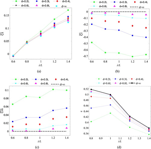
Figure 7(d) shows the curves of power extraction efficiency η varied with λ at different d. For low clearance d (=0.2L and 0.3L), the η first increases with increasing λ and a peak value appeared at λ = 1.0L then decrease with further increasing of λ. When d>0.3L, the η decreases monotonously with increasing λ. The data dispersion degree of η increases with decreasing λ. This trend indicates that the wall effect on η increases with decreasing λ. Compared with the situation of out of wall effect, η decreased due to the presence of wall effect within the parameter testing range. Thus, the fish with smaller wavelength swim near the wall has lower efficiency.

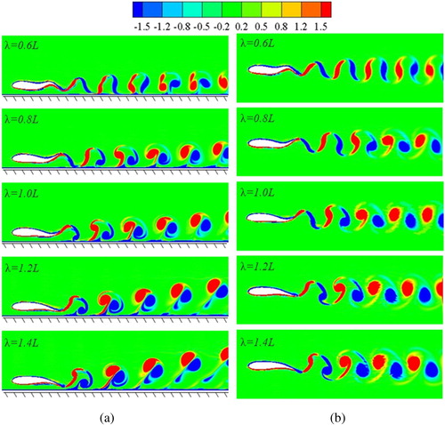
 Figure 8 exhibits the vorticity distribution under different wavelength λ. Compared with the case of out of wall effect at d = 10L (shown in Figure 8(a)), the vortex structures show obvious changes due to the existence of sidewall(show in Figure 8(b)). Similar to the effect of St, at low λ (=0.6L and 0.8L), the vortex shed from the undulating foil becomes shorten and stronger due to the wall effect. As λ keeps increasing, the vortex becomes stronger and stronger and arrayed in pairs in the wake. Besides, we can also find that the vortices move gradually far away from the sidewall and the angle between the sidewall and the centerline of the vortex street increase with increasing λ. This result also proves the phenomenon that the wall effect on fish hydrodynamic force increases with increasing λ.

Figure 8. Vorticity distribution under difference wavelength λ at (a) d = 0.2L and (b) d = 10L.

3.3. Time evolution of the force

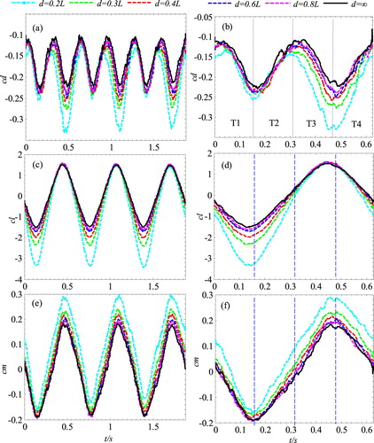
In order to further reveal the wall effect on swimming performance of the fishlike foil, the detail hydrodynamics curves are examined in this study. The time-varying cd, cl, and cm are calculated with the parameters of St = 0.32 and λ = 1L. As shown in Figure 9, periodical trends are observed in all hydrodynamics curves. Particularly, cl and cm curves show the same frequency as undulating movement (see Figure 9(c,e)) and cd curve represents twice the frequency as undulating movement(see Figure 9(a)). The amplitude of the three hydrodynamics curves decreases rapidly when d increasing from 0.2L to 0.3L and then decrease slowly with increasing d, which demonstrates that the wall has a significant effect on the hydrodynamics of the fishlike foil when d ≤ 0.3L and becomes weaker with increasing d. For detailed analysis of the hydrodynamic characteristics, the hydrodynamic curves of single period (see Figure 9(b,d,f)) are divided into four time stages, T1(0T to T/4), T2(T/4 to T/2), T3(T/2 to 3T/4) and T4(3T/4 to T). In stage T1, the cd gradually increased to the first peak and the cl and cm negative growth to the negative peak. Then, the cd decreased to the minimum value, and the cl and cm positive growth to near zero in stage T2. Next, the cd increased again to the second peak while the cl and cm continue positive growth to the positive peak in stage T3. Finally, in stage T4, the cd decreased to the minimum value again, and the cl and cm negative growth to around zero. It can be observed that the second peak of cd is larger than the first one. The amplitude of the cd curve increased with decreasing d in stage T3, and all curves gradually merge in stage T4, which demonstrates that the wall effect on thrust improving occurred in stage T3 and disappeared in stage T4. Moreover, we can also conclude that the wall effect on cl occurred in stage T1 and T4 and gradually disappeared in stage T2 and T3, and a reverse phenomenon can be found for cm curves.

Figure 9. The time-varying (a)(b) drag coefficient cd, (c)(d) lift coefficient cl and (e)(f) moment coefficient cm.

3.4. Flow field around the undulating fishlike foil

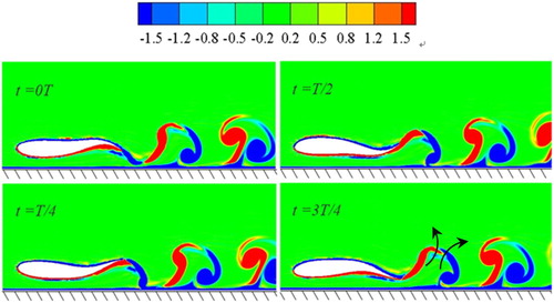
For better understanding the variation of hydrodynamics and power extraction efficiency, we analyzed the flow field distribution around the fishlike foil in detail. Figure 10 provides the vorticity distribution at four moments in one undulating cycle at d = 0.2L, λ = 1L and St = 0.32. At 0T (T is the undulating period), the foil tail oscillates upward and a CW tailing edge vortex (TEV) induced by the tail, then it moves on to T/4, the CW TEV shedding from the tail and impinges on the sidewall. At T/2, the foil tail oscillates downward, and a CCW TEV appeared in the tip of the foil tail. Finally, the CCW TEV shedding from the tail when time goes on to 3T/4. Due to the presence of sidewall, the CW TEV moves slowly to the wake, but the flowing CCW TEV quickly shedding from tail tip. Therefore, both vortices are close together and form a jet between the vortices. Under the effect of the jet, the vortices that arrayed in pairs move gradually far away from the sidewall. Furthermore, we can also find that the CW TEV attached to the foil tail obviously shorter than the CCW TEV in TEV formation stage. The position of CW vortex center in y-axis direction is changed due to the wall effect. According to the Equation (19), the position y also has contribution for the thrust and it further explained the result that the wall has the effect of thrust improving.

Figure 10. Vorticity distribution in one undulating cycle.

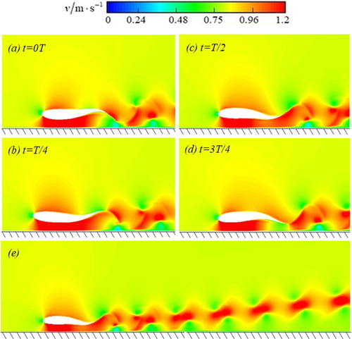
 Figures 11 and 12 show the pressure and velocity contours distribution around the fishlike foil in one undulating period, respectively. The simulation parameters are set as d = 0.2L, λ = 1L and St = 0.32. As shown in Figure 11, a high-pressure area is formed in front of fishlike foil head, and a low-pressure area appeared between the lower surface of foil and sidewall in the whole undulating cycle. This phenomenon can be explained by the Navier-Stokes equation (Chorin, 1968), which demonstrates that the fluid pressure and velocity are negatively correlated. When the fluid flows through the foil, the velocity decreased and formed a low-velocity area in front of the foil due to the resistance of the foil (as shown in Figure 12), correspondingly, the fluid pressure increased and a high-pressure area appeared in front of the foil head. Moreover, the fluid is expelled by foil when it continues moving forward and accelerates to both sides of the foil. Owing to the presence of the sidewall, the fluid velocity between the foil lower surface and the sidewall is increased. Thus, a high-velocity (see Figure 12) and low pressure (see Figure 11) area occurs between the foil lower surface and the sidewall.

Figure 11. Pressure contours distribution around the fishlike foil.

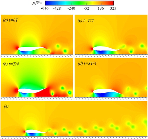
Figure 12. Velocity contours distribution around the fishlike foil.

The pressure difference between both sides of the fishlike foil is the reason for force generating. Here, we further analyze the pressure distribution to reveal the mechanism of force generation. As can be seen in Figure 11(a), the foil tail oscillates upward (moving away from the sidewall according to Figure 1) at 0T and a high and low-pressure area distributes on the upper and lower surfaces along the foil tail respectively. With the tail fin oscillates upward, the cd increased, cl and cm negative growth corresponding to stage T1 in Figure 9(b,d,f). Then, the foil tail oscillates to the maximum amplitude position and begin oscillates downward at T/4 (see Figure 11(b)), the low-pressure center shedding from the foil tail tip and the pressure distribution along the foil tail opposite to the time 0T. The cd reaches the first peak value and the cl and cm achieve the maximum negative value. With the foil tail oscillates downward, the cd turn to decrease, and the cl and cm change to positive growth corresponding to stage T2 in Figure 9(b,d,f). Time goes on to T/2, and a new low-pressure center appeared in the foil tail tip (see Figure 11(c)). The cd reaches the minimum value, and the cl and cm almost equal zero. With the foil tail continues oscillates downward, the cd turn to increase again but the cl and cm continue positive growth corresponding to stage T3 in Figure 9(b,d,f). Finally, at 3T/4, the low-pressure center shedding from the foil tail tip. The foil tail reaches another maximum amplitude position and ready to oscillate upward. The cd increases to the second peak value, and the cl and cm increase to maximum positive value. With the foil tail oscillates upward, the following force variation corresponding to stage T4 in Figure 9(b,d,f). Furthermore, a whole nephogram of pressure field is showed in Figure 11(e), as can be seen, a series of low-pressure center flows that arrayed in pairs shed to the wake and move far away from the sidewall due to the presence of wall effect. Comprehensive analysis of Figures 9 and 11, we can found that the wall effect on cd mainly occurred in stage T3, i.e. foil oscillates downward to the maximum amplitude position from the middle position. The wall effect on the cl occurred in stage T1 and T4, i.e. foil oscillates downward process while for cm appeared in T2 and T4, i.e, foil oscillates downward process.

For the velocity filed, we can also find that a series of high and low alternating arranged velocity center flows appeared in the wake, as shown in Figure 12(e), and gradually move far away from the sidewall due to the wall effect.

4. Conclusions

A numerical simulation of the wall effect on the hydrodynamics performance of a flexible fishlike foil was carried out in this paper. An immersed boundary-lattice Boltzmann method was employed to conduct the simulation for high Reynolds number fluid flow. We examine the influences of the wall effect on the hydrodynamics and flow behaviors of the fishlike foil systematically. The effect of Strouhal numbers St and wavelength λ were especially considered.

The results show that affected by the sidewall, the hydrodynamics and flow behaviors of the fishlike foil show some differences. The wall effect on thrust, lift and moment coefficients increase with increasing of Strouhal numbers and wavelength, but it is opposite for the power extraction efficiency. As compared with the case of out of wall effect, the wall effect has a function of improving thrust, lift and moment. The clearance d has a significant influence on the power extraction efficiency. In some cases (d ≥ 0.6L, st < 0.25), the wall effect improves power extraction efficiency, but in other specific cases (d < 0.6L), it reduces power extraction efficiency. The fish with smaller wavelength, lower Strouhal numbers and swimming closer to the sidewall has lower power extraction efficiency. Moreover, interacting with the sidewall, the vortex becomes shorter and stronger, which is the reason for thrust improving. Finally, all simulations are conducted based on a 2D model in this study, while the real applications are 3D model. Wall effects based on 3D mode are more complex and required to thoroughly investigate in future work.

Acknowledgments

This research is financially supported by Science and Technology Planning Project of Suzhou, China (Grant no.SNG2017054), National Natural Science Foundation of China (Grant no. 51875380) and National Natural Science Foundation of China (Grant no.51805346).

Disclosure statement

No potential conflict of interest was reported by the author(s).

Additional information

Funding

This research is financially supported by Science and Technology Planning Project of Suzhou, China [grant number SNG2017054], National Natural Science Foundation of China [grant number 51875380] and National Natural Science Foundation of China [grant number 51805346].

References

- Anderson, J. M., Streitlien, K., Barrett, D. S., & Triantafyllou, M. S. (1998). Oscillating foils of high propulsive efficiency. Journal of Fluid Mechanics, 360, 41–72. https://doi.org/10.1017/S0022112097008392
- Barrett, D. S., Triantafyllou, M. S., Yue, D. K. P., Grosenbaugh, M. A., & Wolfang, M. J. (1999). Drag reduction in fish-like locomotion. Journal of Fluid Mechanics, 392, 183–212. https://doi.org/10.1017/S0022112099005455
- Blevins, E. L., & Lauder, G. V. (2012). Rajiform locomotion: Three-dimensional kinematics of the pectoral fin surface during swimming in the freshwater stingray Potamotrygon orbignyi. The Journal of Experimental Biology, 215(18), 3231–3241. https://doi.org/10.1242/jeb.068981
- Blevins, E. L., & Lauder, G. V. (2013). Swimming near the substrate: A simple robotic model of stingray locomotion. Bioinspiration & Biomimetics, 8(1), 016005. https://doi.org/10.1088/1748-3182/8/1/016005
- Borazjani, I., & Sotiropoulos, F. (2008). Numerical investigation of the hydrodynamics of carangiform swimming in the transitional and inertial flow regimes. The Journal of Experimental Biology, 211(10), 1541–1558. https://doi.org/10.1242/jeb.015644
- Breder, C. M. (1926). The locomotion of fishes. Zoologica, 4, 159–256.
- Chorin, A. J. (1968). Numerical solution of the Navier-Stokes equations. Mathematics of Computation, 22(104), 745–762. https://doi.org/10.1090/S0025-5718-1968-0242392-2
- Clark, R. P., & Smits, A. J. (2006). Thrust production and wake structure of a batoid-inspired oscillating fin. Journal of Fluid Mechanics, 562(562), 415–429. https://doi.org/10.1017/S0022112006001297
- Coulliette, C., & Plotkin, A. (1996). Aerofoil ground effect revisited. The Aeronautical Journal, 2, 65–74. https:///doi.org/10.1017/S0001924000027305.
- Fernández-Prats, R., Raspa, V., Thiria, B., & Godoy-Diana, R. (2015). Large-amplitude undulatory swimming near a wall. Bioinspiration & Biomimetics, 10(1), 016003. https://doi.org/10.1088/1748-3190/10/1/016003
- Gao, T., & Lu, X. Y. (2008). Insect normal hovering flight in ground effect. Physics of Fluids, 20(8), 087101. https://doi.org/10.1063/1.2958318
- Gazzola, M., Argentina, M., & Mahadevan, L. (2014). Scaling macroscopic aquatic locomotion. Nature Physics, 10(10), 758–761. https://doi.org/10.1038/nphys3078
- Ghalandari, M., Bornassi, S., Shamshirband, S., Mosavi, A., & Chau, K. W. (2019). Investigation of Submerged structures’ flexibility on sloshing frequency using a boundary element method and finite element analysis. Engineering Applications of Computational Fluid Mechanics, 13(1), 519–528. https://doi.org/10.1080/19942060.2019.1619197
- Guo, Z., Zheng, C., & Shi, B. (2002). Discrete lattice effects on the forcing term in the lattice Boltzmann method. Physical Review E, 65(4), 046308. https://doi.org/10.1103/PhysRevE.65.046308
- Hou, S., Sterling, J., Chen, S., & Doolen, G. (1996). A lattice Boltzmann subgrid model for high Reynolds number flows. Fields Institute Communications, 6, 151–166.
- Ji, F., & Huang, D. (2017). Effects of Reynolds number on energy extraction performance of a two dimensional undulatory flexible body. Ocean Engineering, 142, 185–193. https://doi.org/10.1016/j.oceaneng.2017.07.005
- Lighthill, M. J. (1969). Hydrodynamics of aquatic animal propulsion Locomotion. Annual Review of Fluid Mechanics, 1(1), 413–446. https://doi.org/10.1146/annurev.fl.01.010169.002213
- Liu, H., & Kawachi, K. (1999). A numerical study of undulatory swimming. Journal of Computational Physics, 155(2), 223–247. https://doi.org/10.1006/jcph.1999.6341
- Liu, N., Peng, Y., Liang, Y., Liang, Y., & Lu, X. Y. (2012). Flow over a traveling wavy foil with a passively flapping flat plate. Physical Review E, 85(5), 056316. https://doi.org/10.1103/PhysRevE.85.056316
- McNamara, G. R., & Zanetti, G. (1988). Use of the Boltzmann equation to simulate lattice-gas automata. Physical Review Letters, 61(20), 2332–2335. https://doi.org/10.1103/PhysRevLett.61.2332
- Mittal, R., & Iaccarino, G. (2005). Immersed boundary methods. Annual Review of Fluid Mechanics, 37(1), 239–261. https://doi.org/10.1146/annurev.fluid.37.061903.175743
- Mivehchi, A., Dahl, J., & Licht, S. (2016). Heaving and pitching oscillating foil propulsion in ground effect. Journal of Fluids and Structures, 63, 174–187. https://doi.org/10.1016/j.jfluidstructs.2016.03.007
- Molina, J., & Zhang, X. (2011). Aerodynamics of a heaving airfoil in ground effect. AIAA Journal, 49(6), 1168–1179. https://doi.org/10.2514/1.J050369
- Moored, K. W., Dewey, P. A., Boschitsch, B. M., Smits, A. J., & Haj-Hariri, H. (2014). Linear instability mechanisms leading to optimally efficient locomotion with flexible propulsors. Physics of Fluids, 26(4), 041905. https://doi.org/10.1063/1.4872221
- Moryossef, Y., & Levy, Y. (2004). Effect of oscillations on airfoils inclose proximity to the ground. AIAA Journal, 42(9), 1755–1764. https://doi.org/10.2514/1.6380
- Peskin, C. S. (2002). The immersed boundary method. Acta Numerica, 11, 479–517. https://doi.org/10.1017/S0962492902000077
- Quinn, D. B., Lauder, G. V., & Smits, A. J. (2014). Flexible propulsors in ground effect. Bioinspiration & Biomimetics, 9(3), 036008. https://doi.org/10.1088/1748-3182/9/3/036008
- Quinn, D. B., Moored, K. W., Dewey, P. A., & Smits, A. J. (2014). Unsteady propulsion near a solid boundary. Journal of Fluid Mechanics, 742, 152–170. https://doi.org/10.1017/jfm.2013.659
- Rohr, J. J., Hendricks, E. W., Quiqley, L., Fish, F. E., Gilpatrick, J. W., & Scardina-Ludwig, J. (1998). Observations of Dolphin swimming speed and Strouhal number. Space and naval warfare systems center san diego. California, 92152–95001.
- Roper, D. T., Sharma, S., Sutton, R., & Culverhouse, P. (2011). A review of developments towards biologically inspired propulsion systems for autonomous underwater vehicles. Proceedings of the Institution of Mechanical Engineers – Part M: Journal of Engineering for the Maritime Environment, 225(2), 77–96. https://doi.org/10.1177/1475090210397438
- Rozhdestvensky, K. V. (2006). Wing-in-ground effect vehicles Prog. Aerospace Science, 42(3), 211–283. https://doi.org/10.1016/j.paerosci.2006.10.001
- Salih, S. Q., Aldlemy, M. S., Rasani, M. R., Ariffin, A. K., Ya, T. M. Y. S. T., Al-Ansari, N., Yaseen, Z. M., & Chau, K. W. (2019). Thin and sharp edges bodies-fluid interaction simulation using cut-cell immersed boundary method. Engineering Applications of Computational Fluid Mechanics, 13(1), 860–877. https://doi.org/10.1080/19942060.2019.1652209
- Scaradozzi, D., Palmieri, G., Costa, D., & Pinelli, A. (2017). BCF swimming locomotion for autonomous underwater robots: A review and a novel solution to improve control and efficiency. Ocean Engineering, 2017(130), 437–453. https://doi.org/10.1016/j.oceaneng.2016.11.055
- Smagorinsky, J. (1963). General circulation experiments with the primitive equations part I: The basic experiment. Monthly Weather Review, 91(1), 99–165. https://doi.org/10.1175/1520-0493(1963)091<0099:GCEWTP>2.3.CO;2
- Srinidhi, N. G., & Vengadesan, S. (2017). Ground effect on tandem flapping wings hovering. Computers and Fluids, 152(18), 40–56. https://doi.org/10.1016/j.compfluid.2017.04.006
- Tanida, Y. (2001). Ground effect in flight. JSME, 44, 481–486. https://doi.org/10.1299/jsmeb.44.481.
- Triantafyllou, G. S., Triantafyllou, M. S., & Grosenbaugh, M. A. (1993). Optimal thrust development in oscillating foils with application to fish propulsion. Journal of Fluids and Structures, 7(2), 205–224. https://doi.org/10.1006/jfls.1993.1012
- Triantafyllou, M. S., Triantafyllou, G. S., & Yue, D. K. P. (2000). Hydrodynamics of fishlike swimming. Annual Review of Fluid Mechanics, 32(1), 33–53. https://doi.org/10.1146/annurev.fluid.32.1.33
- Truong, T. V., Byun, D., Kim, M. J., Yoon, K. J., & Park, H. C. (2013). Aerodynamic forces and flow structures of the leading edge vortex on a flapping wing considering ground effect. Bioinspiration & Biomimetics, 8(3), 036007. https://doi.org/10.1088/1748-3182/8/3/036007
- Videler, J. J., & Hess, F. (1984). Fast continuous swimming of two pelagic predators, saithe (Pollachius virens) and mackerel (Scomber scombrus): A kinematic analysis. The Journal of Experimental Biology, 109, 209–228.
- Webb, P. W. (2002). Kinematics of plaice, Pleuronectes platessa, and cod, Gadus morhua, swimming near the bottom. The Journal of Experimental Biology, 205(14), 2125–2134.
- Wu, J., Shu, C., & Zhao, N. (2014). Fluid dynamics of flapping insect wing in ground effect. Journal of Bionic Engineering, 1(1), 52–60. https://doi.org/10.1016/S1672-6529(14)60019-6
- Wu, J., Yang, S. C., & Shu, C. (2015). Ground effect on the power extraction performance of a flapping wing biomimetic energy generator. Journal of Fluids and Structures, 54, 247–262. https://doi.org/10.1016/j.jfluidstructs.2014.10.018
- Zhu, Y., & Yu, Y. L. (2017). Thrust-enhancement of an undulating two-dimensional batoid-like model near a flat ground. Journal of University of Chinese Academy of Sciences, 34(1), 23–31. https://doi.org/10.7523/j.issn.2095-6134.2017.01.004