Machine learning versus linear regression modelling approach for accurate ozone concentrations prediction

Abstract

High level of tropospheric ozone concentration, exceeding allowable level has been frequently reported in Malaysia. This study proposes accurate model based on Machine Learning algorithms to predict Tropospheric ozone concentration in major cities located in Kuala Lumpur and Selangor, Malaysia. The proposed models were developed using three-year of historical data for different parameters as input to predict 24-hour and 12-hour of tropospheric ozone concentration. Different Machine Learning algorithms have been investigated, viz. Linear Regression, Neural Network and Boosted Decision Tree. The results revealed that wind speed, humidity, Nitrogen Oxide, Carbon Monoxide and Nitrogen Dioxide have significant influence on ozone formation. Boosted Decision Tree outperformed Linear regression and Neural Network algorithms for all stations. The performance of the proposed model improved by using 12-hours dataset instead of the 24-hour where R² values were equal to 0.91, 0.88 and 0.87 for the three investigated stations. To assess the uncertainties of the Boosted Decision Tree model, 95% prediction uncertainties (95PPU) d-factors were introduced.95PPU showed about 94.4, 93.4, 96.7% and the d-factors were 0.001015, 0.001016 and 0.001124 which relate to S1, S2 and S3, respectively. The obtained results provide a reliable prediction model to mimic actual ozone concentration in different locations in Malaysia.

KEYWORDS:

• Ozone concentration prediction
• machine learning algorithm
• ozone precursors
• Boosted Decision Tree Regression
• neural network
• linear regression
• Pearson Correlation

1. Introduction

Ozone is a gas made up of three oxygen atoms (O₃) where it occurs naturally in small amount in the stratosphere (upper atmosphere) which help to protect life on Earth from the sun's ultraviolet (UV) radiation. Tropospheric Ozone located at lower atmosphere is a major air pollutant in urban areas that include metropolitan cities like Kuala Lumpur, Petaling Jaya and Kelang in Malaysia. When present in sufficient quantity, tropospheric ozone can have severe effects on humans’ health such as respiratory and cardiovascular diseases (Zhan et al., 2018). It is imperative to examine both indoor and outdoor ozone concentration to monitor ambient air quality (Shen et al., 2017); (Chen et al., 2018). Moreover, tropospheric ozone gives negative impact toward crops production and vegetation in general (Antanasijević et al., 2019); (Ismail et al., 2011). In Malaysia, regulations have been set by the Department of Environment (DOE) known as New Malaysia Ambient Air Quality Standard to limits the emission of air pollutants concentration in such a way that they cannot exceed recommended maximum values since 1989. New Malaysia Ambient Air Quality Standard for ground level ozone, O₃ cannot exceed the average of 1-hour time by 2020 standard which will be 200 $\text{μ}g/{\text{m}}^3$ or average of 8-hour time by 2020 standard of 120 $\text{μ}g/{\text{m}}^{\text{3}}$ (‘Official Portal of Department of Environment’, 2019). Malaysia is a developing country and Kuala Lumpur, Petaling Jaya and Kelang are the major cities thus susceptible to high-ozone concentration generated due to air pollution from fuel combustion, generation of Volatile organic compounds (VOCs) and operation from high industrial zones. Therefore, future increase of ozone concentration need to be carefully monitored (Ezimand & Kakroodi, 2019).

Various methods have been initiated for predicting the ozone concentration all over the world such as deterministic (theoretical and detailed atmospheric diffusion model) and statistical regression (Capilla, 2016; Gao et al., 2018; Hoshyaripour et al., 2016). Some methods have been developed based on linear regression concept. Multiple Linear Regression (MLR) is one of the most popular linear regression methods in predicting ozone concentration (Banja et al., 2012; Huang et al., 2019). However, this model shows drawback to apprehend the nonlinearity and complexity associated with the structure of system (Arsić et al., 2020).

Recently Artificial intelligence technique has gained popularity among researchers as a nonlinear approach to solve complex problem to forecast air quality (Abdul-Wahab & Al-Alawi, 2002; Alimissis et al., 2018). Over the years, improvements have been made toward neural network model to provide a robust prediction model (Biancofiore et al., 2015). Recurrent architecture significantly improves the performance of neural predictors by only using meteorological parameters as input data. Moreover, recent study to develop hybrid model based on convolutional neural network and long short-term memory (CNN-LSTM) provided a satisfactory hybrid model for seasonal stability and its prediction performance proved to be superior than multilayer perceptron (MLP) and LSTM (Pak et al., 2018). Self-adaptive neuro-fuzzy weighted extreme learning machine to improve prediction accuracy and real-time air pollution concentration prediction has been investigated by (Li et al., 2018). On the other hand, recently many researchers implemented Support Vector Machines (SVMs) to predict ozone concentration in an advance time-series manner (Luna et al., 2014). The modified SVM-r model is flexible enough to encompass other input variable such as city models or traffic patterns that might enhance prediction. Few studies focused on prediction ozone concentration in urban areas (Abdullah et al., 2019; Pawlak & Jarosławski, 2019; Shaban et al., 2016). However, no one has investigated the robustness of Boosted Decision Tree Regression in predicting ozone concentrations in general and specifically in urban cities.

Developing an accurate prediction model requires the selection of the input parameters, such as air quality and meteorological data, that have impacts on the changes in ozone concentration (Gómez-Losada et al., 2018; Gradišar et al., 2016; Ragosta et al., 2015; Zhang et al., 2019). However, most of the desirable data are often unavailable or incomplete due to the problem of data source retrieval or large missing data (Gómez-Sanchis et al., 2006; Hájek & Olej, 2012). Therefore, there is need to develop model with high level of precision by using few input parameters.

In this study four models – Boosted Decision Tree Regression (BDTR), Neural Network with Gaussian Normalizer, Neural Network with Min–Max Normalizer and Linear Regression – with six different input parameters are investigated. Pearson Correlation Coefficient was used to select proper input parameters to the proposed models. These models then tested at three different location in Malaysia. Two different scenarios were investigated were the accuracy of the proposed model tested by predicting the ozone concentrations for different time horizon, 24-hour and 12-hour. The models’ performances are then compared to evaluate their robustness by implementing various performance. Finally, as for the best model, the uncertainties are assessed by using the indices of bracketed by the 95PPU and d-factor.

2. Materials and methods

2.1. Study area and dataset

The area of investigation covers Kuala Lumpur and Selangor, Malaysia. In Kuala Lumpur the monitoring station is located at SMK. Seri Permaisuri Cheras $({3.1070}^{\circ }\text{N},{101.7177}^{\circ }\text{E})$ which is denoted as S1. The Selangor first monitoring station is located at SK. Bandar Utama Petaling Jaya $({3.1383}^{\circ }\text{N},{101.6097}^{\circ }\text{E})$ and known as S2 and second monitoring station of Selangor is located at SMK(P). Raja Zarina Kelang $({3.010998}^{\circ }\text{N},{101.409622}^{\circ }\text{E})$ and denoted as S3. Selangor surrounds the federal territories of Kuala Lumpur and Putrajaya. Hence, both areas of investigation are on the west coast of Peninsular Malaysia (Figure 1).

Figure 1. Location of monitoring stations.

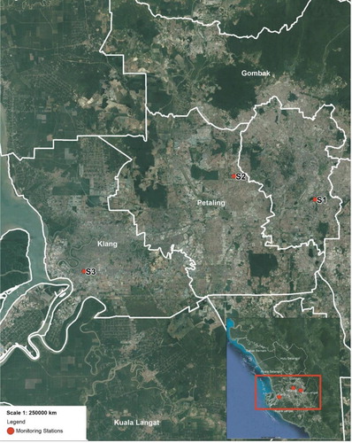
The land surface in Selangor is leveled on the west and hilly on the east. The climate is very much dictated by the surrounding sea and prevailing wind system with tropical rainforest climate, high average temperature and high average rainfall. January is the benchmark of highest precipitation throughout the year whereas the lowest precipitation is on October. Although January has the highest precipitation, the temperature is still moderately high. Hottest temperature is on June reaching up to 37°C and the lowest temperature is on November.

Selangor and Kuala Lumpur are considered as highly populated regions in Malaysia due to the development of Klang Valley, started in 1980. Rapid development is seen over the years in the regions not only focusing on building structures but with good infrastructure facilities. However, driving own vehicle is still preferable by most of the citizens to commute from one place to another.

Monitoring stations provide air quality and meteorological data which were obtained from the Department of Environment (DOE). The original dataset includes hourly average wind speed (WS), Humidity (HUM), Nitrogen Oxide (NO_x), Sulphur Dioxide (SO₂), Nitrogen Dioxide (NO₂), Ozone (O₃) and Carbon Monoxide (CO). These datasets are historical data of three years’ observation from 1st of January 2012 until 31st December 2014.

In this study the datasets were first analyzed then sorted into two categories for three years of historical data used for the areas under investigation. First category was hourly average of 24 h with a total of 1,84,128 data as given in Table 1. Second category was hourly average daytime only from 6:00 am to 6:00 pm with total of 92,064 data as given in Table 2.

Table 1. Statistics of 24-hours raw data.

	S1							S2							S3
Statistics/study location	WS	HUM	NOx	SO2	NO2	O3	CO	WS	HUM	NOx	SO2	NO2	O3	CO	WS	HUM	NOx	SO2	NO2	O3	CO
Maximum	17.3	100	0.187	0.075	0.077	0.17	4.13	22	100	0.302	0.059	0.094	0.116	6.62	19.2	100	0.292	0.111	0.093	0.122	14.03
Minimum	0.8	26	0.001	0	0.001	0	0	1	28	0	0	0	0	0	1	20	0	0	0	0	0
Mean	3.438	93.533	0.036	0.002	0.021	0.020	0.809	4.804	70.043	0.061	0.004	0.029	0.014	1.194	5.895	69.164	0.037	0.004	0.021	0.018	1.149
Mean Deviation	2.354	8.393	0.019	0.001	0.008	0.019	0.385	1.892	13.724	0.026	0.002	0.009	0.013	0.484	2.467	10.132	0.020	0.003	0.009	0.013	0.555
Sample Standard Deviation	2.785	10.877	0.024	0.002	0.011	0.024	0.490	2.408	15.952	0.034	0.003	0.012	0.016	0.634	3.028	12.205	0.027	0.005	0.012	0.016	0.832
Median	2.4	100	0.03	0.001	0.019	0.009	0.69	4.4	71	0.055	0.003	0.027	0.007	1.09	5.1	70	0.03	0.003	0.02	0.012	0.93

Table 2. Statistics of 12- hour daylight raw data.

	S1							S2							S3
Statistics/study location	WS	HUM	NOx	SO2	NO2	O3	CO	WS	HUM	NOx	SO2	NO2	O3	CO	WS	HUM	NOx	SO2	NO2	O3	CO
Maximum	17.3	100	0.16	0.042	0.063	0.17	3.77	21.2	100	0.302	0.059	0.087	0.116	6.62	18.3	100	0.24	0.111	0.079	0.122	11.43
Minimum	0.8	26	0.001	0	0.001	0	0	1	28	0	0	0	0	0	1	20	0	0	0	0	0
Mean	4.385	89.703	0.029	0.002	0.017	0.029	0.671	5.563	65.469	0.055	0.004	0.026	0.020	1.106	7.034	66.066	0.033	0.005	0.018	0.023	1.035
Mean Deviation	2.452	10.560	0.016	0.001	0.007	0.022	0.326	1.981	14.065	0.023	0.002	0.008	0.016	0.453	2.702	11.005	0.019	0.003	0.008	0.015	0.531
Sample Standard Deviation	2.906	12.614	0.021	0.002	0.009	0.027	0.424	2.518	16.205	0.030	0.003	0.011	0.019	0.608	3.224	13.006	0.026	0.007	0.011	0.018	0.810
Median	4.2	97	0.023	0.001	0.015	0.024	0.55	5.3	63	0.051	0.003	0.025	0.015	1	6.6	65	0.026	0.003	0.017	0.02	0.79

In order to get optimum results, any missing data in each column was cleaned by using the function of clean missing data with cleaning mode of replace using Probabilistic principal components analysis (PCA). The cleaned dataset was normalized by using Lognormal transformation method. This is applied though all numeric columns used in the model. Normalization is imperative as part of data preparation to create new values within the general distribution and ratios subsequently maintain the values in the source data. Both dataset categories were split into training set and testing set. With randomly selected data, 75% of the total data were for training and 35% was for testing.

2.2. Input selection for sensitivity test

Filter-based feature selection is an essential step in performing machine-learning algorithm model. It was used to identify the columns in input dataset that have the greatest predictive power. In this study, the Pearson Correlation was used for filter selection metric. Pearson Correlation measures the linear correlation between two variables X and Y that is called Pearson Correlation Coefficient. It is the covariance of the two variables divided by the product of their standard deviations. Any changes of the scale in the two variables will not affect the Pearson Correlation Coefficient.

Pearson Correlation: (1) $r_{xy}=\frac{\sum _{i=1}^n(x_i-\overline{x})(y_i-\overline{y})}{\sqrt{\sum _{i=1}^n{(x_i-\overline{x})}^2}\sqrt{\sum _{i=1}^n{(y_i-\overline{y})}^2}}$(1) $r_{xy}$ is the covariance; correlation function, n is the sample size of the data. x_i, y_i are the individual sample points indexed with i. $\overline{x}$ and $\overline{y}$ sample mean.

2.3. Models selections

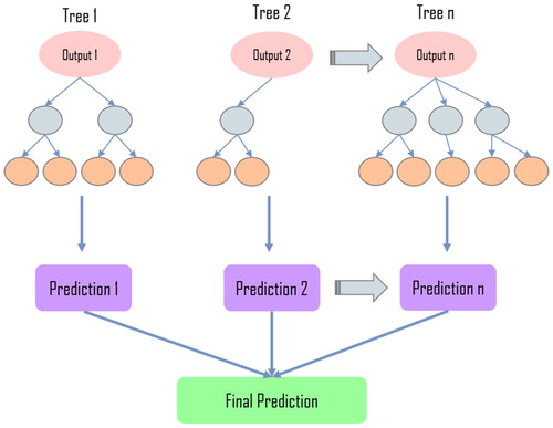
A set of statistical analysis was used to compare the performance of each algorithm. This includes Boosted Decision Tree Regression. Boosted Decision Tree regression is an algorithm used to train the model by implementing MART (Multiple Additive Regression Trees) algorithm. Each tree is dependent on the prior tress, that is how boosting works as shown in Figure 2. In each step the loss function will be defined to measure the error in order to crrect the next tree till the optimum tree obtained. Therefore, in Boosted Decision Tree regression, prediction is an ensemble of group of weaker prediction models that come together to form a strong prediction model as shown in below formula: (2) $\begin{array}{rl}\hat{y}(x)& =\sum _t{w}_t{h}_t(x)\end{array}$(2) (3) $\begin{array}{rl}O(x)& =\sum _{i}l({\hat{y}}_i,y_i+\sum _t\mathrm{\Omega }(f_t)\end{array}$(3) Whereby h(x) is the tree's output, wis the weight, $l({\hat{y}}_i,y_i)$ is the loss function, distance between the truth and the prediction of ith sample. $\mathrm{\Omega }(f_t)$ is a regularization function.

Figure 2. Typical boosted decision tree regression structure.

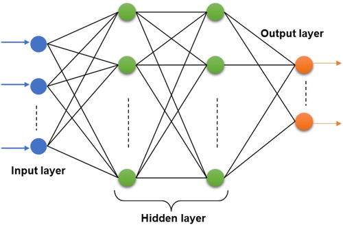
The Neural Network Regression Algorithm was used next. The Neural network is usually used in classification and regression problems. Neural network model consists of three arranged layers as shown in Figure 3. The principle is that hidden layer will transforms input data into high dimensional space whereby each neuron in the hidden layer apply radial function. All hidden neurons are connected to the output neurons by adjusting output weights at the last layer of output layer (Ali Ghorbani et al., 2018; Homsi et al., 2019; Qasem et al., 2019).

Figure 3. Simple neural network model.

Finally, comparision between the proposed model and Linear Regression Algorithm was carried out in this study. Linear regression shows a linear relationship between one or more independent variables and a numeric dependent variable outcome.

Linear Regression: (4) $y=\alpha +\beta x$(4) Where $\beta$ is the slope of line and $\alpha$ is y-intercept for linear relationship between $\gamma$ and x regression.

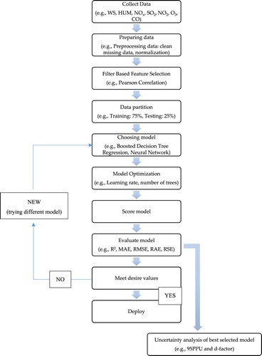
Figure 4 shows the steps of the proposed method in this study. Several performance indexes used to validate the scored model on how close the computed ozone concentrations to the real values, which can be given as follows:

1. Coefficient of determination, R². High R² value indicate good model performance. (5) $R^2=\frac{\sum _{i=1}^n{(y_i-{\overline{Y}}_i)}^2-\sum _{i=1}^n{(y_i-{\hat{y}}_i)}^2}{\sum _{i=1}^n{(y_i-{\overline{y}}_i)}^2}$(5)

   Figure 4. Flow chart of the prediction methodology of 3-year historical hourly average ozone concentration using machine learning algorithms.

   

2. Mean absolute error, MAE measures accuracy of continuous variables. (6) $MAE=\frac{1}{n}\sum _{i=1}^n|y_i-{\hat{y}}_i|$(6)

3. Root mean square error, RMSE whereby $y_i$and ${\hat{y}}_i$ are the observation and prediction in the i-th step. RMSE and MAE are responsible to measure the residual error and are imperative to indicate the output unit error. (7) $RMSE=\sqrt{\frac{1}{n}\sum _{i=1}^n{(y_i-{\hat{y}}_i)}^2}$(7)

4. Relative absolute error, RAE. The relative absolute error is the normalized value by dividing the total absolute error to the simple predictor total absolute error. (8) $RAE=\frac{\sum _{i=1}^n|{\hat{y}}_i-y_i|}{\sum _{i=1}^n\overline{y}-{y_i}^2}$(8)

5. Relative square error, RSE. The relative square error is the normalized value by dividing the total square error to the simple predictor total square error. (9) $RSE=\frac{\sum _{i=1}^n{({\hat{y}}_i-y_i)}^2}{\sum _{i=1}^n{(\overline{y}-y_i)}^2}$(9)

2.4. Uncertainty analysis of best selected model

Uncertainty analysis attempts to measure the output variance due to input variability. It is carried out to define the range of possible outcomes based on input uncertainty and to examine the impact of the model's lack of knowledge or errors. This study employ the technique, 95% of projected uncertainties (95PPU), advocated by Abbaspour (Noori et al., 2010). 95PPU is computed by percentiles of 2.5% X_L and 97.5% X_U. (10) $\begin{array}{rl}& \text{Bracketed by }95PPU\\ & =\frac{1}{k}\text{count}(K|X_L\le K\le X_U)\times 100\end{array}$(10) Whereby k is the number of observed data at testing stages. Based on Eq. (10), the value of ‘Bracketed by 95PPU’ is maximum (or 100%) when all measured data at testing stages are inserted between the X_L and X_U. The acceptable range of the measured data should fall between 80–100% in the 95PPU level. However, in case of some regions where data are poor, 50% of data in 95PPU would be appropriate (Noori et al., 2010). In addition, d-factor parameter is used to estimate the average width of confidence interval band as shown in Eq. (11). (11) $\text{d}-\text{factot}=\frac{{\overline{\text{d}}}_x}{{\sigma }_x}$(11) ${\sigma }_x$ is the standard deviation of the measured data (x) and ${\overline{\text{d}}}_x$ is the average distance between the upper and lower bands as in Eq. (12). (12) ${\overline{\text{d}}}_x=\frac{1}{k}\sum _{i=1}^k(X_U-X_L)$(12)

3. Results and discussion

The study aimed to explore the capability of different machine learning algorithm models for the prediction of hourly average ozone concentration at any desirable time in Kuala Lumpur and Selangor. Then all these models were optimized by analyzing the prediction accuracy in terms of performance indexes.

3.1. Pearson correlation coefficient

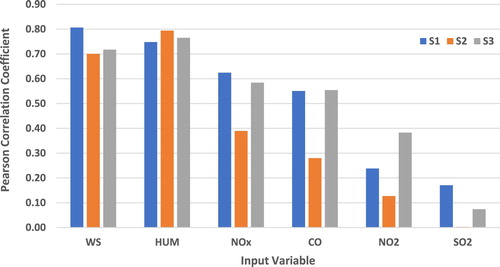
Pearson Correlation Coefficient is used to measure how related each of the parameters to the dependent variable. Based on Figure 5, it can be seen that there are four parameters that have high correlation with dependent variable which is Ozone. For example, at S1, the highest Pearson correlation coefficient found to be with wind speed followed by humidity, nitrogen oxide and finally carbon monoxide. Such correlation is reported by other studies which found Ozone concentration to be affected by the wind velocity in terms of horizontal transport and vertical mixing (‘Official Portal of Department of Environment’, 2019); (Fang et al., 2019). At S2 and S3 the result show that humidity is the highest parameter correlated with dependent variable followed by wind speed, nitrogen oxide and last carbon monoxide. Nitrogen dioxide shows the lowest correlation with dependent variable at all monitoring stations. Finally, Sulphur dioxide shows the least correlation with almost no impact with the output variable especially for the model at S2.

Figure 5. Bar chart of Pearson correlation coefficient of input variable with output variable, O³ (6:00 am – 6:00 pm).

3.2. Models performance at each monitoring stations

Table 3 indicates the performance indices for training dataset of the four models based at three monitoring stations for both scenarios 24-hour and daytime 12-hour. The Boosted Decision Tree Regression model shows that when only 12- hour daytime is considered instead of 24-hour dataset, high level of coefficient of determination (R²) values were obtained for all stations. The 12- hour daytime dataset R² value for S1 is 0.91977, for S2 is 0.88439 and for S3 is 0.87859 whilst 24-hour dataset has R² of 0.85985 for S1, 0.78897 for S2 and 0.80631 for S3. The presence of sunlight during the day hence help ozone formation. This explains why 12-hour daytime models outperformed the 24-hour models. Other performance indices such as the Mean absolute error (MAE), Root Mean square error (RMSE), Relative Absolute error (RAE) and Relative Square Error (RSE) confirmed the accuracy of the proposed model as presented in Table 3.

Table 3. Performance indexes of training dataset.

Training		24-h					12-h (6:00 am – 6:00 pm)
Algorithm	Station	R^2	MAE	RMSE	RAE	RSE	R^2	MAE	RMSE	RAE	RSE
Boosted Decision Tree Regression	1	0.860	0.085	0.119	0.296	0.140	0.920	0.060	0.085	0.227	0.080
	2	0.789	0.113	0.152	0.375	0.211	0.884	0.075	0.107	0.266	0.116
	3	0.806	0.100	0.134	0.367	0.194	0.879	0.076	0.103	0.294	0.121
Neural Network Regression: Gaussian Normalizer	1	0.768	0.116	0.153	0.405	0.232	0.822	0.091	0.127	0.343	0.178
	2	0.689	0.144	0.185	0.477	0.311	0.801	0.102	0.141	0.360	0.199
	3	0.712	0.124	0.164	0.458	0.288	0.761	0.107	0.144	0.415	0.239
Linear Regression	1	0.746	0.126	0.160	0.440	0.254	0.791	0.107	0.138	0.402	0.209
	2	0.670	0.150	0.191	0.497	0.330	0.765	0.117	0.153	0.412	0.235
	3	0.703	0.130	0.166	0.479	0.297	0.742	0.118	0.150	0.460	0.258
Neural Network Regression: Min-Max Normalizer	1	0.744	0.126	0.161	0.440	0.256	0.787	0.109	0.139	0.409	0.213
	2	0.703	0.140	0.181	0.464	0.297	0.758	0.121	0.155	0.426	0.242
	3	0.680	0.137	0.172	0.504	0.320	0.741	0.119	0.150	0.461	0.259

Moreover, the Boosted Decision Tree Regression models outperformed all other models including the Neural Network regression with Gaussian Normalizer, Linear Regression and Neural Network with Min–Max Normalizer. In terms of accuracy, Neural Network with Gaussian Normalizer represents the second best then followed by the Linear Regression and finally Neural Network Regression. The Min–max Normalizer was the lowest in its accuracy to predict 12-hour daytime Ozone concentrations.

After the training of all models using training dataset, the unseen data were used to test the models. Table 4 displays the performance indices for testing dataset for the four models based on the three monitoring stations. Again, boosted decision tree regression model exhibits higher R² values for 12-hour daytime dataset compared to 24-hour dataset of all stations. Daytime dataset R² value of S1 is 0.87350, for S2 is 0.82166 and for S3 is 0.81143, whereas 24-hour dataset R² value of S1 is 0.83670, for S2 is 0.74163 and for S3 is 0.76737. The difference between daytime and 24-hour R² value is noticeably high thus prove daytime data significantly improve prediction model capability.

Table 4. Performance indexes for testing dataset.

Testing		24-h					12-h (6:00 am – 6:00 pm)
Algorithm	Station	R^2	MAE	RMSE	RAE	RSE	R^2	MAE	RMSE	RAE	RSE
Boosted Decision Tree Regression	1	0.837	0.093	0.129	0.321	0.163	0.874	0.074	0.108	0.275	0.127
	2	0.742	0.126	0.170	0.413	0.258	0.822	0.092	0.133	0.325	0.178
	3	0.767	0.109	0.146	0.402	0.233	0.811	0.093	0.129	0.357	0.189
Neural Network Regression: Gaussian Normalizer	1	0.781	0.114	0.149	0.397	0.219	0.827	0.090	0.126	0.333	0.173
	2	0.699	0.143	0.184	0.470	0.301	0.794	0.103	0.143	0.363	0.206
	3	0.720	0.123	0.161	0.453	0.280	0.764	0.107	0.144	0.410	0.236
Linear Regression	1	0.761	0.124	0.156	0.430	0.239	0.798	0.105	0.136	0.391	0.202
	2	0.676	0.150	0.191	0.493	0.324	0.763	0.117	0.153	0.412	0.237
	3	0.711	0.129	0.163	0.476	0.289	0.743	0.119	0.151	0.454	0.257
Neural Network Regression: Min-Max Normalizer	1	0.758	0.124	0.157	0.430	0.242	0.795	0.108	0.137	0.399	0.205
	2	0.710	0.140	0.180	0.458	0.290	0.759	0.121	0.155	0.426	0.241
	3	0.685	0.135	0.170	0.500	0.315	0.743	0.119	0.151	0.455	0.257

Moving on to other models that include Neural Network Regression with Gaussian Normalizer, Linear Regression and Neural Network Regression with Min–Max Normalizer exhibit the same trend as the Boosted decision tree Regression which is for daytime dataset has higher R² values compared to 24-hour dataset. Performance indexes such as the MAE, RMSE, RAE and RSE also show lower values. Therefore, according to Table 4, it can be concluded that the Boosted Decision Tree Regression represents the best model for daylight compared to other models. The rank from highest to lowest performance for the other models is similar with the training dataset given in Table 3. The Neural Network with Gaussian Normalizer is ranked as the second-best model followed by Linear Regression and Neural Network with Min–Max Normalizer was the lowest.

Over the years, there has been many studies done to design the best model to predict ozone concentration. The most popular methods are Support Vector Machine (SVM) by (Luna et al., 2014), the typical artificial neural network by (Gao et al., 2018). Based on past research by (Gao et al., 2018) the performance index for ANN modeling in testing phase was R² equal to 0.859 whilst the proposed model of BDTR in this study shown R² equal to 0.920 and 0.874 for training and testing, respectively. The finding of this study reveals that the BDTR outperformed ANN and it can be used as reliable model in predicting the concentrations of Ozone in urban cities.

3.3. Taylor diagram

Taylor diagram provides a summary of how fit the patterns match of their correlation, root-mean-square difference and variance ratio [34]. Construction of Taylor diagram is based on the formula as follows: (13) $R=\frac{\frac{1}{N}\sum _{n=1}^N(f_n-\overline{f})(r_n-\overline{r})}{{\sigma }_f{\sigma }_r}$(13) Whereby the R is the correlation coefficient, N is the number of discrete points, $f_n\text{and}{r}_n$ are two variables, ${\sigma }_f\text{and}{\sigma }_r$ is the standard deviation of f and r and $\overline{f}\text{and}\overline{r}$ are the mean values of ${\sigma }_f\text{and}{\sigma }_r$.

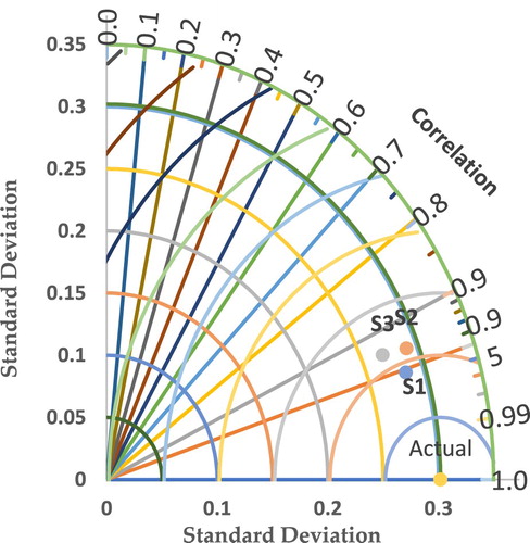
Figure 6 illustrates the relationship between the standard deviation $(\sigma )$ and correlation (R) of predicted ozone and actual ozone at each location for all models. It can be seen that in all stations the proposed model M1 has a better correlation with the actual ozone compared with other models. In addition, the standard deviation for the predicted ozone from M1 is closer to standard deviation of actual ozone which indicates that the proposed model is consistent in predicting the value of concentration for entire population of the data as shown in Figure 7.

Figure 6. Taylor diagram measures of model correlation and standard deviation with actual ozone.

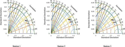
Figure 7. Taryor diagram for Boosted Decision Tree Regression on each site.

3.4. Optimization of Boosted Decision Tree Regression (BDTR)

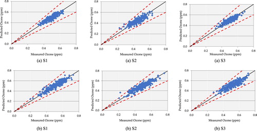
The proposed BDTR models were then optimized in order to improve the model accuracy by tuning the hyper-parameter such as learning rate and number of trees. Figure 8 reveals the relationship between the performance of the models represented by the correlation coefficient, the learning rate, and the number of trees at the three locations. The best correlation coefficient was obtained when the learning rate is 0.8 for the three investigated locations during the training phase where it was equal to 0.97213 at S1, 0.95835 at S2 and 0.95748 at S3. While the optimum number of trees was found when the learning rate is high for all the locations and it is exponentially decreased until a lowest value is achieved. Figure 9 presents the scatterplots of predicted versus measured ozone concentrations. It can be seen that the optimized Boosted Decision Tree Regression models is capable to precisely mimicking the actual data during the testing phase for all locations of 24-hour and 12-hour scenarios.

Figure 8. Correlation Coefficient Vs Number of Trees Vs Learning Rate: S1, S2 and S3.

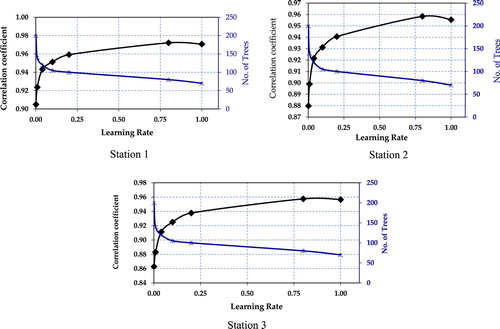
Figure 9. Scatter plot of predicted versus measured ozone for: (a) 24-hour testing dataset and (b) daylight testing dataset for.

3.5. Uncertainty analysis of Boosted Decision Tree Regression model

Uncertainty analysis of the best model Boosted Decision Tree was calculated 95PPU and d-factor. Table 5 represents the uncertainty analysis results for the stations using the 12-hour testing dataset.

Table 5. Uncertainty analysis of BDTR model.

Station	Statistic	BDTR
1	L95PPU	−0.077798
	U95PPU	94.419011
	d- factor	0.001015
2	L95PPU	−3.628877
	U95PPU	93.393741
	d- factor	0.001016
3	L95PPU	−2.631008
	U95PPU	96.657048
	d- factor	0.001124

The values bracketed by 95PPU indicate that about 94.4%, 93.4% and 96.7% of data for the best Boosted Decision Tree model relate to S1, S2 and S3, respectively. Moreover, the d-factor has values of 0.001015, 0.001016 and 0.001124 for S1, S2 and S3, respectively. From this results it can be concluded that the proposed model showed outstanding performance for predicting the ozone concentration in this study area. However, in order to generalize the performance of the proposed model to another study area required further analysis for the historical records of the ozone concentration. This is due to the fact that each case study has its own pattern of the ozone concentration pattern that might need further adjustment in the model architecture.

4. Conclusions

The capability of the Boosted Decision Tree Regression model was assessed based on the available historical data measured from 2012 to 2014. The proposed Boosted Decision Tree Regression models were then optimized based on the learning rate and total number of trees constructed. The study showed that Boosted Decision Tree outperformed Linear regression and Neural Network algorithms for all stations. The performance of the proposed model improved by using 12-hours dataset instead of the 24-Hours where R² values were equal to 0.91977, 0.88439 and 0.87859 for the three stations, respectively. The findings provide a promising base for conducting further investigations on the robustness of the Boosted Decision Tree Regression model for ozone concentration prediction in different time horizon. Additionally, the reliability of the Boosted Decision Tree Regression was evaluated based on uncertainty estimation using 95PPU and d-factor indices. It is seen that the Boosted Decision Tree model has an acceptably low degree of uncertainty. In this study, high level of accuracy was obtained using only few meteorological variables (such as wind speed, humidity, Nitrogen Oxide, Carbon Monoxide and Nitrogen Dioxide) as input to the proposed model. However, further studies might be needed to improve the proposed model by introducing more input parameters which have not been investigated due to the lack of such information. In addition, introducing more advanced optimization algorithm to be integrated with the Boosted Decision Tree Regression models might improve the prediction accuracy and accelerate the convergence rate.

Acknowledgments

The authors would like to acknowledge the Ministry of Higher Education Malaysia providing a fundamental research grant scheme No: FRGS/1/2018/TK10/UNITEN/03/2. In addition, the authors would like to thank the Malaysian Meteorological Department (MetMalaysia) for providing relevant data.

Disclosure statement

No potential conflict of interest was reported by the author(s).

Additional information

Funding

This work was supported by Ministry of Higher Education Malaysia providing a fundamental research grant: [Grant Number FRGS/1/2018/TK10/UNITEN/03/2].

References

- Abdul-Wahab, S. A., & Al-Alawi, S. M. (2002). Assessment and prediction of tropospheric ozone concentration levels using artificial neural networks. Environmental Modelling and Software, 17(3), 219–228. https://doi.org/10.1016/S1364-8152(01)00077-9
- Abdullah, S., Nasir, N. H. A., Ismail, M., Ahmed, A. N., & Jarkoni, M. N. K. (2019). Development of ozone prediction model in urban area. International Journal of Innovative Technology and Exploring Engineering, 8(10), 2263–2267. https://doi.org/10.35940/ijitee.J1127.0881019
- Ali Ghorbani, M., Kazempour, R., Chau, K.-W., Shamshirband, S., & Ghazvinei, P. T. (2018). Forecasting pan evaporation with an integrated artificial neural network quantum-behaved particle swarm optimization model: A case study in Talesh, Northern Iran. Engineering Applications of Computational Fluid Mechanics, 12(1), 724–737. https://doi.org/10.1080/19942060.2018.1517052
- Alimissis, A., Philippopoulos, K., Tzanis, C. G., & Deligiorgi, D. (2018). Spatial estimation of urban air pollution with the use of artificial neural network models. Atmospheric Environment, 191, 205–213.https://doi.org/10.1016/j.atmosenv.2018.07.058
- Antanasijević, D., Pocajt, V., Perić-Grujić, A., & Ristić, M. (2019). Urban population exposure to tropospheric ozone: A multi-country forecasting of SOMO35 using artificial neural networks. Environmental Pollution, 244, 288–294. https://doi.org/10.1016/j.envpol.2018.10.051
- Arsić, M., Mihajlović, I., Nikolić, D., Živković, Ž., & Panić, M. (2020). Prediction of ozone concentration in ambient air using multilinear regression and the artificial neural networks methods. Ozone: Science & Engineering, 42(1), 79–88. https://doi.org/10.1080/01919512.2019.1598844
- Banja, M., Papanastasiou, D. K., Poupkou, A., & Melas, D. (2012). Development of a short-term ozone prediction tool in tirana area based on meteorological variables. Atmospheric Pollution Research, 3(1), 32–38.https://doi.org/10.5094/APR.2012.002
- Biancofiore, F., Verdecchia, M., Di Carlo, P., Tomassetti, B., Aruffo, E., Busilacchio, M., Bianco, S., Di Tommaso, S., & Colangeli, C. (2015). Analysis of surface ozone using a recurrent neural network. Science of the Total Environment, 514, 379–387. https://doi.org/10.1016/j.scitotenv.2015.01.106
- Capilla, C. (2016). Prediction of hourly ozone concentrations with multiple regression and multilayer perceptron models. International Journal of Sustainable Development and Planning, 11(4), 558–565. https://doi.org/10.2495/sdp-v11-n4-558-565
- Chen, S., Mihara, K., & Wen, J. (2018). Time series prediction of CO2, TVOC and HCHO based on machine learning at different sampling points. Building and Environment, 146, 238–246. https://doi.org/10.1016/j.buildenv.2018.09.054
- Ezimand, K., & Kakroodi, A. A. (2019). Prediction and spatio – Temporal analysis of ozone concentration in a metropolitan area. Ecological Indicators, 103, 589–598. https://doi.org/10.1016/j.ecolind.2019.04.059
- Fang, C., Wang, L., & Wang, J. (2019). Analysis of the spatial–temporal variation of the surface ozone concentration and its associated meteorological factors in Changchun. Environments, 6(4), 46. https://doi.org/10.3390/environments6040046
- Gao, M., Yin, L., & Ning, J. (2018). Artificial neural network model for ozone concentration estimation and Monte Carlo analysis. Atmospheric Environment, 184, 129–139. https://doi.org/10.1016/j.atmosenv.2018.03.027
- Gómez-Losada, Á., Asencio–Cortés, G., Martínez–Álvarez, F., & Riquelme, J. C. (2018). A novel approach to forecast urban surface-level ozone considering heterogeneous locations and limited information. Environmental Modelling and Software, 110, 52–61. https://doi.org/10.1016/j.envsoft.2018.08.013
- Gómez-Sanchis, J., Martín-Guerrero, J. D., Soria-Olivas, E., Vila-Francés, J., Carrasco, J. L., & del Valle-Tascón, S. (2006). Neural networks for analysing the relevance of input variables in the prediction of tropospheric ozone concentration. Atmospheric Environment, 40(32), 6173–6180. https://doi.org/10.1016/j.atmosenv.2006.04.067
- Gradišar, D., Grašič, B., Zlata Božnar, M., Mlakar, P., & Kocijan, J. (2016). Improving of local ozone forecasting by integrated models. Environmental Science and Pollution Research, 23(18), 18439–18450. https://doi.org/10.1007/s11356-016-6989-2
- Hájek, P., & Olej, V. (2012). Ozone prediction on the basis of neural networks, support vector regression and methods with uncertainty. Ecological Informatics, 12, 31–42. https://doi.org/10.1016/j.ecoinf.2012.09.001
- Homsi, R., Shiru, M. S., Shahid, S., Ismail, T., Harun, S. B., Al-Ansari, N., Chau, K.-W., & Yaseen, Z. M. (2019). Precipitation projection using a CMIP5 GCM ensemble model: A regional investigation of Syria. Engineering Applications of Computational Fluid Mechanics, 14(1), 90–106. https://doi.org/10.1080/19942060.2019.1683076
- Hoshyaripour, G., Brasseur, G., Andrade, M. F., Gavidia-Calderón, M., Bouarar, I., & Ynoue, R. Y. (2016). Prediction of ground-level ozone concentration in São Paulo, Brazil: Deterministic versus statistic models. Atmospheric Environment, 145, 365–375. https://doi.org/10.1016/j.atmosenv.2016.09.061
- Huang, Y., Yang, Z., & Gao, Z. (2019). Contributions of indoor and outdoor sources to ozone in residential buildings in Nanjing. International Journal of Environmental Research and Public Health, 16(14), 2587. https://doi.org/10.3390/ijerph16142587
- Ismail, M., Suroto, A., Ibrahim, T. A. E., & Abdullah, A. M. (2011). Tropospheric ozone trend in the Muda irrigation area, Kedah. Journal of Physical Science, 22(2), 87–99.
- Li, Y., Jiang, P., She, Q., & Lin, G. (2018). Research on air pollutant concentration prediction method based on self-adaptive neuro-fuzzy weighted extreme learning machine. Environmental Pollution, 241, 1115–1127. https://doi.org/10.1016/j.envpol.2018.05.072
- Luna, A. S., Paredes, M. L. L., de Oliveira, G. C. G., & Corrêa, S. M. (2014). Prediction of ozone concentration in tropospheric levels using artificial neural networks and support vector machine at Rio de Janeiro, Brazil. Atmospheric Environment, 98, 98–104.https://doi.org/10.1016/j.atmosenv.2014.08.060
- Noori, R., Hoshyaripour, G., Ashrafi, K., & Araabi, B. N. (2010). Uncertainty analysis of developed ANN and ANFIS models in prediction of carbon monoxide daily concentration. Atmospheric Environment, 44(4), 476–482. https://doi.org/10.1016/j.atmosenv.2009.11.005
- “Official Portal of Department of Environment.” (2019).
- Pak, U., Kim, C., Ryu, U., Sok, K., & Pak, S. (2018). A hybrid model based on convolutional neural networks and long short-term memory for ozone concentration prediction. Air Quality, Atmosphere and Health, 11(8), 883–895. https://doi.org/10.1007/s11869-018-0585-1
- Pawlak, I., & Jarosławski, J. (2019). Forecasting of surface ozone concentration by using artificial neural networks in rural and urban areas in Central Poland. Atmosphere, 10(2), 52. https://doi.org/10.3390/atmos10020052
- Qasem, S. N., Samadianfard, S., Kheshtgar, S., Jarhan, S., Kisi, O., Shamshirband, S., & Chau, K.-W. (2019). Modeling monthly pan evaporation using wavelet support vector regression and wavelet artificial neural networks in arid and humid climates. Engineering Applications of Computational Fluid Mechanics, 13(1), 177–187. https://doi.org/10.1080/19942060.2018.1564702
- Ragosta, M., D’Emilio, M., & Giorgio, G. A. (2015). Input strategy analysis for an air quality data modelling procedure at a local scale based on Neural Network. Environmental Monitoring and Assessment, 187(5). https://doi.org/10.1007/s10661-015-4556-9
- Shaban, K. B., Kadri, A., & Rezk, E. (2016). Urban air pollution monitoring system with forecasting models. IEEE Sensors Journal, 16(8), 2598–2606. https://doi.org/10.1109/JSEN.2016.2514378
- Shen, J., Chen, J., Zhang, X., Zou, S., & Gao, Z. (2017). Outdoor and indoor ozone concentration estimation based on artificial neural network and single zone mass balance model. Procedia Engineering, 205, 1835–1842. https://doi.org/10.1016/j.proeng.2017.10.253
- Zhan, Y., Luo, Y., Deng, X., Grieneisen, M. L., Zhang, M., & Di, B. (2018). Spatiotemporal prediction of daily ambient ozone levels across China using random forest for human exposure assessment. Environmental Pollution, 233, 464–473. https://doi.org/10.1016/j.envpol.2017.10.029
- Zhang, J., Wang, C., Qu, K., Ding, J., Shang, Y., Liu, H., & Wei, M. (2019). Characteristics of ozone pollution, regional distribution and causes during 2014–2018 in Shandong Province, East China. Atmosphere, 10(9), 501. https://doi.org/10.3390/atmos10090501