Comparative analysis of hybrid models of firefly optimization algorithm with support vector machines and multilayer perceptron for predicting soil temperature at different depths

Abstract

This research aims to model soil temperature (ST) using machine learning models of multilayer perceptron (MLP) algorithm and support vector machine (SVM) in hybrid form with the Firefly optimization algorithm, i.e. MLP-FFA and SVM-FFA. In the current study, measured ST and meteorological parameters of Tabriz and Ahar weather stations in a period of 2013–2015 are used for training and testing of the studied models with one and two days as a delay. To ascertain conclusive results for validation of the proposed hybrid models, the error metrics are benchmarked in an independent testing period. Moreover, Taylor diagrams utilized for that purpose. Obtained results showed that, in a case of one day delay, except in predicting ST at 5 cm below the soil surface (ST5_cm) at Tabriz station, MLP-FFA produced superior results compared with MLP, SVM, and SVM-FFA models. However, for two days delay, MLP-FFA indicated increased accuracy in predicting ST_5cm and ST _20cm of Tabriz station and ST_10cm of Ahar station in comparison with SVM-FFA. Additionally, for all of the prescribed models, the performance of the MLP-FFA and SVM-FFA hybrid models in the testing phase was found to be meaningfully superior to the classical MLP and SVM models.

KEYWORDS:

• Firefly optimization algorithm
• soil temperature
• artificial neural networks
• hybrid machine learning
• prediction

Introduction

Soil temperature (ST) and its spatial and temporal changes directly or indirectly affect the extent and direction of many processes occurring in soil (Mehdizadeh et al., 2018) such as seed germination, root elongation, evaporation, storage and movement of water and microbial activities, nutrient cycle, and many other dynamic processes of the soil (Beltrami, 2001; Citakoglu, 2017; Qian et al., 2011). Soil temperature is affected by several factors, including topography, solar radiation, air temperature, precipitation, soil moisture content and soil thermal conductivity, and heat transfer coefficients (Bilgili, 2010, 2011; Hillel, 1998). ST at various depths may be either directly measured or estimated by air temperature modeling. Therefore, methods that can provide acceptable results may be a suitable solution for estimating ST at the needed locations as well as predicting for subsequent months. The use of artificial neural network models has been widely considered in recent years (Chau & Muttil, 2007; Cheng et al., 2005; Fotovatikhah et al., 2018; Kazemi et al., 2018; Kim & Singh, 2014; Kisi et al., 2015; Mazou et al., 2013; Moazenzadeh et al., 2018; Qasem et al., 2019; Samadianfard et al., 2019; Samadianfard, Ghorbani, et al., 2018; Wu et al., 2013; Yaseen et al., 2019). So far, many studies have been carried out on soil temperature estimation. Using the numerical method, Hanks et al. (1971) estimated ST as a function of time and depth. In this study, the calculated temperature difference was 1.5° C with the actual temperature. Zheng et al. (1993) using air temperature and applying linear regression, estimated ST at a depth of 10 cm under six climate types in the United States. For ST estimation, Plauborg (2002) offered experimental and straightforward relationships. The outcomes revealed that the experimental model with a correlation coefficient of 0.98 could predict ST precisely. Gill et al. (2006) applied SVM for ST estimation and compared its results with the estimations of ANN models. They stated that SVM models achieved better ST estimations than ANN models. Sabziparvar, Tabari, et al. (2010) used multivariate regressions for ST estimation at eight selected meteorological stations of Iran using climatic variables. The results indicated that RMSE varied from 2.06 to 2.75 (°C). Moreover, Sabziparvar, Zare Abyaneh, et al. (2010) conducted a study on ST soil temperature estimation at Zahedan and Ramsar stations using multivariate regression. In the best and worst cases, the correlation coefficient was 0.94 and 0.64, respectively. Bilgili (2010) compared regression and artificial neural network models in predicting ST. A neural network with a precision of 0.998 (°C) has more exceptional performance than regression methods. Using the artificial neural network and monthly meteorological data, Bilgili (2011) predicted ST in the next month. His results exhibited that the neural network is a trustworthy model for predicting soil temperature. Tabari et al. (2011) investigated the performances of ANN for estimating ST values and stated that the estimates by ANN were in better agreement with observations than those by regression methods. Tabari et al. (2015) used the neural network (ANN) and multivariate regression (MLR) using a large number of meteorological variables and estimated soil temperature of up to 100 cm depths at five stations located at a dry desert area of Iran. The results of this study revealed that among the atmospheric variables, average temperature and relative humidity had the most significant effects on soil temperature. Samadianfard, Asadi, et al. (2018) investigated the effectiveness of wavelet neural networks (WNN) for estimating ST at various depths. Obtained results exposed that the WNN produced more precise predictions. Additionally, they concluded that with increasing soil depth, the estimation accuracy for all methods reduced drastically. Sanikhani et al. (2018) implemented monthly ST estimation utilizing extreme learning machine (ELM), ANN and M5 Model Tree. Obtained results revealed that the ELM model was produced as the most precise estimations of ST compared to the other considered models. In another study, Sihag et al. (2019) examined the precision of MLP, Gaussian Process (GP), Random Forest (RF) and the M5P models in estimating ST_5cm at Tabriz and Ahar stations. They only evaluated the accurateness of the considered models in estimating ST_5cm and stated that MLP had more accurate predictions than others.

Although ST is recognized as an effective variable in environmental and agricultural practices, only a few research works have developed data-driven forecasting models for its prediction. By this basic recognition and a need to perform such research in semi-arid conditions, the contemporary explorations in this area have intended to study the association among ST and other meteorological parameters using novel and innovative hybrid learning models such as SVM-FFA model. The utility of such research is expected to have significant implications in maintaining the ecological sustainability of the environment and empowering agricultural productivity, including a pivotal role in formulating more strategic soil management policies by decision-makers in the agricultural sector.

Considering those mentioned above, the purpose of this study is to: (1) construct and evaluate MLP-FFA and SVM-FFA models in predicting the ST at different depths, (2) apply the mentioned models trained with data from Tabriz and Ahar synoptic stations with meteorological parameters, (3) evaluate different modeling scenarios that represent the different combinations of meteorological parameters established to study their contributory roles in modeling ST at different depths in the study region.

Materials & methods

Multilayer perceptron neural network

The artificial neural network was first presented in 1943 by Mcculloch and Pitts (McClelland & Rumelhart, 1988). Generally, the layered perceptron neural network structure consists of input, output, and hidden layers, each with a different number of neurons. The number of the mentioned layers is related to the nature of the considered problem, and the number of hidden layers is selected by trial and error procedure for minimizing the prediction error (Firat & Gungor, 2009; Ustaoglu et al., 2008). Additionally, the effect of each variable is determined by giving a weight to every neuron of the input layer (Ghorbani et al., 2016) and hyperbolic-tangent sigmoid function, Logarithmic sigmoid function, and Linear function were utilized as the activation function for input, hidden and output layers, as presented in equations 1–3, respectively. (1) $\begin{array}{rl}\text{f}\left(\text{x}\right)& =\frac{2}{1+e^{-2\text{x}}}-1\end{array}$(1) (2) $\begin{array}{rl}\text{f}\left(\text{x}\right)& =\frac{1}{1+e^{-\text{x}}}\end{array}$(2) (3) $\begin{array}{rl}\text{f}\left(\text{x}\right)& =x\end{array}$(3)

Support vector machines

Support vector machine (SVM), as one of the learning methods, is resulted from statistical learning theory (Vapnik, 1995). The mentioned method utilizes a decision surface for splitting target classes by maximizing their margins (Burges, 1998). This decision surface is typically called an optimum hyperplane and the nearest data point to this plane are named support vectors. Notably, these support vectors are vital elements of the training process. The form of the SVM model is described as following: (4) $\text{f}\left(\text{x}\right)=w^{\text{T}}x+b$(4) where w and b represent the coefficients of the weight vector.

Firefly algorithm

Yang (2008) presented an optimization technique based on the movement of fireflies and named it as ‘firefly algorithm’ (Ghorbani et al., 2017; Yang, 2008). Fireflies live in nature as in colonies and always a firefly with less light travels toward the light and brilliant firefly (Gazi & Passino, 2004). The brightness is proportional to the distance from the source and attractiveness changes with absorption (Fister et al., 2013). (5) $I\left(r\right)=\frac{I_s}{r^2}$(5) In the above relation r is the distance, $I_s$ is the intensity of the light source, for an environment with a constant light gain coefficient γ the intensity of light I change with r (Fister et al., 2013). (6) $I=I_0{e}^{-\gamma r}$(6) That I₀ is the intensity of the original light.

Because the attraction of a firefly is relative to the observed light intensity by the nearby fireflies, we can define the charm of β as follows (Fister et al., 2013): (7) $\text{β}={\text{β}}_0{e}^{-\gamma r^2}$(7) That β₀ is the charm in r = 0.

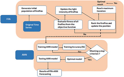
In a real implementation, the charm function β(r) can be any descending uniform function, as in the following general form (Fister et al., 2013): (8) $B\left(r\right)={\text{β}}_0{e}^{-\gamma r^m}$(8) It should be noted that for improving the performance of ST estimations, FFA was utilized for selecting optimized values of the SVM parameters. So, Figure 1 shows the FFA algorithm based on the ANN model.

Figure 1. Hybridization of the firefly algorithm based on artificial neural network.

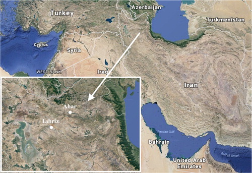
Study area

This study was performed using data from Tabriz and Ahar stations (Figure 2), located in East Azerbaijan province, Iran. The mentioned province is positioned in the range of ${45}^{\circ }{07}^{\mathrm{\prime }}$ to ${48}^{\circ }{20}^{\mathrm{\prime }}$ east longitude and ${36}^{\circ }{45}^{\mathrm{\prime }}$ to ${39}^{\circ }{26}^{\mathrm{\prime }}$ north latitude and is ranked first in the northwest of Iran regarding agriculture production.

Figure 2. Location of the studied stations (URL1).

The meteorological variables studied in this research are listed in Table 1. Moreover, typical earth thermometers were utilized for measuring ST values at different depths.

Table 1. Meteorological variables used in the proposed models.

Variables	Notation
Air temperature (°C)	T
Wind speed (m/s)	W
Relative Humidity (%)	RH
Sunshine hours (hr)	SUN
ST at 5 cm below the surface (°C)	ST5cm
ST at 10 cm below the surface (°C)	ST10cm
ST at 20 cm below the surface (°C)	ST20cm

Table 2 depicts the statistical parameters of all data. It comprehended from this table that T, ST and RH show normal distributions with low skewness values. Also, the correlation coefficients between meteorological parameters and ST values presented in Table 3. The air temperature and relative humidity have the most significant direct and inverse correlations with ST values, respectively. Figure 3 demonstrates the ST variations at all depths.

Figure 3. variations of measured ST at different depths.

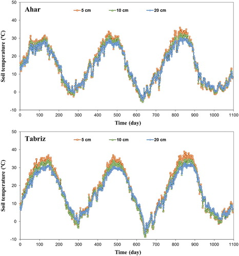
Table 2. Statistical characteristics of used data.

	Variables*	skewness	Stretch index	Mean	Min	Max	Standard deviation
Tabriz	T	−0.21	−0.9	13.58	−13	32.2	10.26
	SUN	−0.78	−0.45	8.01	0	13.5	3.74
	RH	0.23	−1.03	51.18	14.12	94.37	18.21
	W	0.73	0.012	3.7	0	10.62	1.71
	ST5cm	0.005	−1.31	17.42	−8.13	39	12.43
	ST10cm	−0.04	−1.32	16.51	−8.57	34.93	11.7
	ST20cm	−0.06	−1.33	16.19	−6.73	32.67	10.38
Ahar	T	−0.29	−0.82	11.67	−13.5	28.2	8.62
	SUN	−0.59	−0.77	7.42	0	13/6	3.91
	RH	0.28	−0.48	58.21	22.62	97	15.28
	W	1.21	1.24	3.25	0	15.75	1.71
	ST5cm	0.095	−1.36	14.88	−5.27	35.93	11.22
	ST10cm	0.48	−1.39	14.63	−5.53	32.8	10.59
	ST20cm	0.004	−1.42	14.27	−4.6	30.13	9.82

*For the units see Table 1.

Table 3. Correlation coefficients between ST and meteorological variables.

	ST	T	W	RH	SUN
Tabriz	ST5cm	0.957	0.506	−0.782	0.658
	ST10cm	0.964	0.499	−0.783	0.656
	ST20cm	0.970	0.484	−0.779	0.650
Ahar	ST5cm	0.806	−0.139	−0.384	0.439
	ST10cm	0.821	−0.142	−0.387	0.443
	ST20cm	0.843	−0.152	−0.392	0.447

Evaluation criteria

For evaluating the prediction accuracy of the studied models, root mean squared error (RMSE), mean absolute error (MAE), and correlation coefficient (R) were utilized as presented in equations 9–11. Additionally, the Taylor diagram, which is a graphical evaluation design, was used to confirm the accurateness of considered models. In the Taylor diagram, several aspects can be reviewed instantly (Gleckler et al., 2008; Taylor, 2001). (9) $\begin{array}{rl}\text{RMSE}& =\sqrt{\frac{\sum _{\text{i}=1}^{\text{n}}{({\text{p}}_{\text{i}}-{\text{o}}_{\text{i}})}^2}{\text{n}}}\end{array}$(9) (10) $\begin{array}{rl}\text{MAE}& =\frac{\sum _{\text{i}=1}^{\text{n}}|{\text{p}}_{\text{i}}-{\text{o}}_{\text{i}}|}{\text{n}}\end{array}$(10) (11) $\begin{array}{rl}\text{R}& =\frac{\sum _{\text{i}}^{\text{n}}\left({\text{o}}_{\text{i}}-\overline{\mathrm{o}}\right)\left({\text{p}}_{\text{i}}-\overline{\mathrm{p}}\right)}{\sqrt{\sum _{\text{i}=1}^{\text{n}}{\left({\text{o}}_{\text{i}}-\overline{\mathrm{o}}\right)}^2\sum _{\text{i}=1}^{\text{n}}{\left({\text{p}}_{\text{i}}-\overline{\mathrm{p}}\right)}^2}}\end{array}$(11)

Where ${\text{p}}_{\text{i}}$ is the ith predicted value by models, ${\text{o}}_{\text{i}}$ is the ith observed value and n is the total number of sample data.

Results and discussion

In the current research, five input arrangements based on meteorological parameters were assembled and evaluated to determine whether the proposed MLP-FFA and SVM-FFA hybrid models were capable of data-driven tools for modeling the soil temperature at different depths with one and two days delay (Table 4). It should be noted that in the case of one day as delay, the current values and in the case of two days as delay, the current and previous correspondent values were implemented. Also, note that the input combination (1) has employed the most highly correlated variable but as a single input only, whereas input combination (2) has incorporated the two most highly direct and inverse correlated variables and input combination (3) has utilized the three most relevant variables. Likewise, input combination (4) has used all variables to model the ST data. The ideal combination of these model inputs aimed to produce accurate models that represented the most substantial variables, as well as a carefully selected combination of these variables to check their influence on the testing performances.

Table 4. Defined input arrangements for ST estimation.

Structure	Input parameters	Output parameters
1	T(t-a)	ST5cm, ST10cm, ST20cm
2	T(t-a), RH(t-a)	ST5cm, ST10cm, ST20cm
3	T(t-a), RH(t-a), SUN(t-a)	ST5cm, ST10cm, ST20cm
4	T(t-a), RH(t-a), SUN(t-a), W(t-a)	ST5cm, ST10cm, ST20cm
5	T(t-a), RH(t-a), W(t-a)	ST5cm, ST10cm, ST20cm

In all models, we followed the notion that there is no rule of thumb for that the universal way the training and testing data partitioned. For example, the study of Kurup and Dudani (2002) used a total of their 63% of data for model development while Pal (2006) applied 69%, Samadianfard et al. (2013) and Samadianfard et al. (2014) used 67% of total data to develop their models. So, the current utilized data parted into training (70%) and testing (30%). In other words, meteorological data of 2013 and 2014 (total of 730) implemented for training the considered models, while the correspondent data of 2015 (total of 365) utilized for testing them. It is imperative to note that trial and error procedures implemented for finding the optimal structures of the models. This followed the fact that there is not any definite verified process for indicating the ideal number of hidden neurons and parameters, and these are typically selected in an iterative manner (Deo & Sahin, 2015, 2017).

Additionally, after examining the different training algorithms and transfer functions, the Levenberg-Marquardt algorithm and the sigmoid transfer function were selected for the current research. Various kernel functions have been analyzed and the optimum kernel for each input combination with optimized hyperparameters was selected based on the error functions. The obtained error meters are presented in Tables 5 and 6.

Table 5. The results of modeling with MLP, SVM, MLP-FFA and SVM-FFA for Tabriz and Ahar stations with a delay of one day at different depths.

			Train			Test
Station	Output parameter	Best model	R^2	MAE (°C)	RMSE (°C)	R^2	MAE (°C)	RMSE (°C)
Tabriz	ST5cm	MLP5	0.92	2.58	3.34	0.95	2.38	3.07
		MLP-FFA5	0.97	1.55	1.93	0.97	1.66	2.18
		SVM1	0.92	2.61	3.33	0.95	2.55	3.15
		SVM-FFA1	0.97	1.68	2.18	0.97	1.59	2.15
	ST10cm	MLP1	0.93	2.25	2.91	0.96	1.90	2.45
		MLP-FFA1	0.99	0.97	1.28	0.98	1.23	1.58
		SVM1	0.93	2.25	2.92	0.96	1.91	2.48
		SVM-FFA1	0.96	1.71	2.21	0.98	1.43	1.85
	ST20cm	MLP5	0.95	1.71	2.25	0.96	1.54	2.01
		MLP-FFA5	0.99	0.90	1.11	0.99	0.92	1.17
		SVM1	0.95	1.79	2.34	0.97	1.61	2.03
		SVM-FFA1	0.97	1.35	1.73	0.98	1.10	1.33
Ahar	ST5cm	MLP3	0.71	4.63	5.75	0.77	4.94	6.05
		MLP-FFA3	0.91	2.39	3.16	0.85	3.81	4.64
		SVM4	0.76	4.26	5.32	0.73	5.17	6.45
		SVM-FFA4	0.91	2.11	2.80	0.84	3.29	4.83
	ST10cm	MLP4	0.88	2.89	4.12	0.78	4.38	5.49
		MLP-FFA4	0.91	2.39	3.08	0.84	3.68	4.51
		SVM4	0.78	3.80	4.80	0.76	4.59	5.75
		SVM-FFA4	0.91	2.00	2.67	0.75	3.43	5.11
	ST20cm	MLP3	0.78	3.68	4.67	0.82	3.45	4.36
		MLP-FFA3	0.84	2.96	3.75	0.87	3.24	3.95
		SVM4	0.81	3.23	4.12	0.79	4.00	5.08
		SVM-FFA4	0.92	1.79	2.41	0.75	0.72	4.88

Table 6 The results of modeling with MLP, SVM, MLP-FFA and SVM-FFA for Tabriz and Ahar stations with a delay of two days at different depths

			Train			Test
Station	Output parameter	Best model	R^2	MAE (°C)	RMSE (°C)	R^2	MAE (°C)	RMSE (°C)
Tabriz	ST5cm	MLP4	0.93	2.37	3.08	0.94	2.55	3.26
		MLP-FFA4	0.98	1.31	1.66	0.98	1.29	1.71
		SVM4	0.94	2.27	2.95	0.94	1.61	3.33
		SVM-FFA4	0.96	1.73	2.26	0.97	1.74	2.36
	ST10cm	MLP1	0.92	2.40	3.11	0.96	2.10	2.63
		MLP-FFA1	0.98	1.30	1.70	0.98	1.41	1.89
		SVM4	0.95	1.99	2.60	0.95	2.15	2.64
		SVM-FFA4	0.98	1.25	1.63	0.98	1.16	1.63
	ST20cm	MLP3	0.95	1.68	2.22	0.96	1.58	2.12
		MLP-FFA3	0.99	0.89	1.11	0.99	0.90	1.15
		SVM4	0.95	1.64	2.17	0.96	1.72	2.21
		SVM-FFA4	0.98	1.01	1.31	0.98	0.88	1.31
Ahar	ST5cm	MLP3	0.73	4.59	5.66	0.74	5.20	6.34
		MLP-FFA3	0.92	2.37	3.06	0.82	4.09	5.03
		SVM4	0.75	4.39	5.46	0.72	6.25	6.59
		SVM-FFA4	0.84	3.32	4.00	0.81	3.84	4.60
	ST10cm	MLP1	0.68	4.72	5.82	0.77	4.64	5.63
		MLP-FFA1	0.82	3.52	4.37	0.86	3.42	4.47
		SVM4	0.77	3.92	4.93	0.75	4.66	5.89
		SVM-FFA4	0.80	3.37	4.20	0.79	3.77	4.73
	ST20cm	MLP3	0.78	3.62	4.47	0.82	3.84	4.71
		MLP-FFA3	0.85	2.92	3.62	0.87	2.85	3.80
		SVM4	0.80	3.34	4.23	0.78	4.09	5.18
		SVM-FFA4	0.88	2.53	3.10	0.86	3.00	3.69

As can be seen from Tables 5 and 6, a comprehensive evaluation has been carried out for revealing the capabilities of the mentioned hybrid models using several statistical meters such as R², MAE and RMSE indices. So, in the case of predicting ST_5cm at Tabriz station, SVM-FFA1 and MLP-FFA4 with RMSE values of 2.15°C and 1.71°C produced better results in the case of one and two days delay, respectively. Also, they improved the accuracies of standalone SVM and MLP models with 31.75% and 47.55%, respectively. However, somehow the reverse trend has been seen in predicting ST_5cm at Ahar station. In this case, MLP-FFA3 and SVM-FFA4 with RMSE values of 4.64°C and 4.60°C, respectively, predicted ST values more precisely than standalone MLP and SVM models with one and two days delay. Also, the improvement percentage of MLP and SVM models were 23.31% and 30.20%, respectively. Thus, it can be comprehended that MLP-FFA4 and SVM-FFA4 with the same meteorological parameters of T, RH, SUN and W provided superior predictions of ST_5cm at Tabriz and Ahar stations. Comparing these obtained results with findings of Sihag et al. (2019) shows that the RMSE values of MLP-FFA4 and SVM-FFA4 (1.71°C and 4.60°C) are lower than the best accurate models of Sihag et al. (2019) (MLP with RMSE of 3.26°C and 6.33°C). So, MLP, GP, RF and the M5P models in estimating ST_5cm are not recommended. Additionally, in the case of predicting ST_10cm, it can be revealed from Tables 5 and 6 that MLP-FFA1, SVM-FFA4 (Tabriz station) and MLP-FFA4, MLP-FFA1 (Ahar station) in the case of one and two days delay and with RMSE values of 1.58°C, 1.63°C, 4.51°C, and 4.47°C predicted ST values more accurately than standalone MLP and SVM models with different input combinations. In other words, they improved the prediction accuracy of standalone MLP and SVM models by 35.51%, 38.26%, 17.85%, and 20.60%, respectively. Conclusively, MLP-FFA1 which only uses the input parameter of T has been selected as the precise model in predicting ST_10cm at both studied stations. Finally, in predicting ST_20cm at Tabriz station, it can be found from Tables 5 and 6 that MLP-FFA5 and MLP-FFA3 with one and two days delay and having the RMSE values of 1.17°C and 1.15°C, respectively, predicted ST values with lower error values than standalone MLP and SVM and other hybrid models with different input combinations. The mentioned MLP-FFA5 and MLP-FFA3 in the prediction of ST_20cm at Tabriz station reduced the RMSE values of correspondent standalone MLP models by 41.79% and 45.75%, respectively.

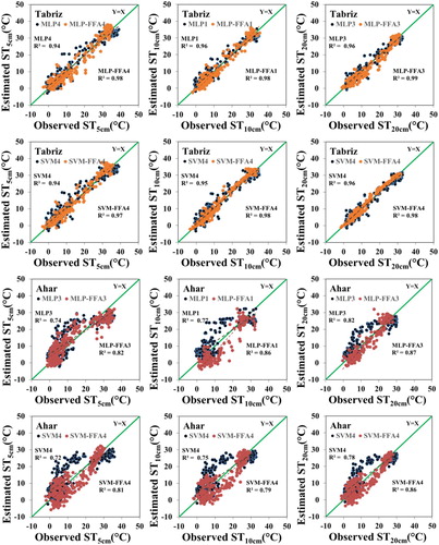
Moreover, at Ahar station, MLP-FFA3 and SVM-FFA4 with one and two days delay, respectively, predicted ST_20cm values more precisely than standalone MLP and SVM models. In other words, the improvement rates of standalone MLP and SVM models, in this case, were 9.40% and 28.76%, respectively. MLP-FFA3 with input parameters of T, RH, SUN and SVM-FFA4 with input parameters of T, RH, SUN, and W in the case of two days delay presented more accurate predictions of ST_20cm values than other hybrid models of MLP and SVM with different input combinations. As a remarkable point, it is clear that forth input combination with parameters of T, RH, SUN, and W is in the majority for selecting as the best input combination for ST predicting at both studied stations. The importance of these factors in estimating soil temperature as the inputs of the model considered. The following graphs (Figures 4 and 5) show the dispersion scattering points at a depth of 5, 10 and 20 cm than modeling with best MLP, SVM and MLP-FFA, SVM-FFA models.

Figure 4. Scatterplots of the estimated-observed ST values by best models with a delay of one day at different depths.

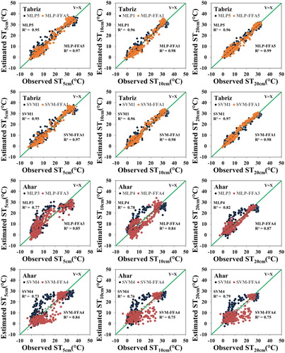
Figure 5. Scatterplots of the estimated-observed ST values by best models with a delay of two days at different depths.

Moreover, the comprehensive comparison between the results of all studied models with one and two days as delay revealed that the accuracy of the best models in the case of two days as delay were higher than the correspondent models with one day as delay except for ST_10cm at Tabriz station. This may be related to the fact that using previous values of meteorological parameters can be useful in increasing the accuracies of the studied models.

Comparing the obtained results with findings of Samadianfard, Asadi, et al. (2018) showed that MLP-FFA1 with one day delay and MLP-FFA3 with tow days delay had better performances in comparison with the best model WNN models in estimating ST_10cm and ST_20cm, respectively. But in the case of ST_5cm, the accuracy of WNN in the study of Samadianfard, Asadi, et al. (2018) was higher than the best FFA integrated model in the current study.

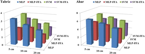
For additional assessing the accuracy of the established models, Figures 4 and 5 present a scatter plot of observed and predicted ST values. Obviously, the R²-value for all panels exposes the higher accuracy of the hybrid models, which agrees with previous results in Tables 5 and 6. Also, Figures 6 and 7 display three-dimensional bar graphs of the RMSE produced by studied hybrid models analyzed using different combinations of meteorological parameters. Agreeing with earlier results interpretations, the predicted ST values at different depths discovered a superior effectiveness of the hybrid models. Additionally, errors produced by hybrid models were expressively lower than those of the classical models (by 9.40% to almost 45.75%).

Figure 6. RMSE bar graph for ST prediction with one day delay.

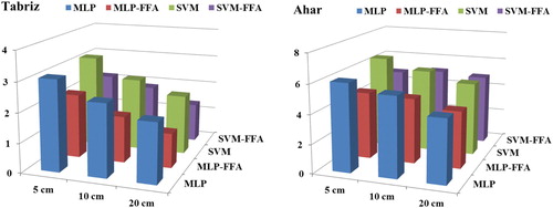
Figure 7. RMSE bar graph for ST prediction with two days delay.

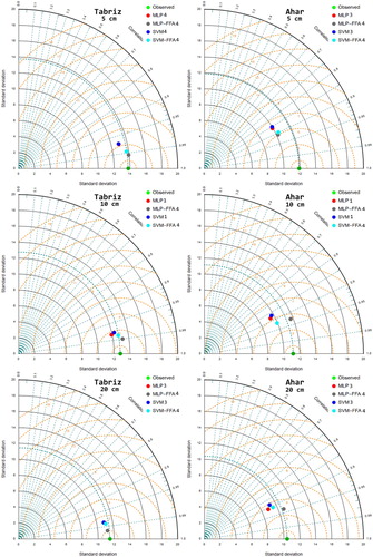
Besides, Taylor diagrams were implemented for exploring the accurateness of hybrid models (Figures 8 and 9). In Taylor's diagrams, the distance from the reference green point is an amount of the centered RMSE (Taylor, 2001). Therefore, an accurate model is selected based on the distance of the correspondent point to the green one. It is clear from Taylor's diagrams that MLP-FFA and SVM-FFA models provided the most precise predictions than standalone MLP and SVM models.

Figure 8. Taylor diagrams (with a delay of one day).

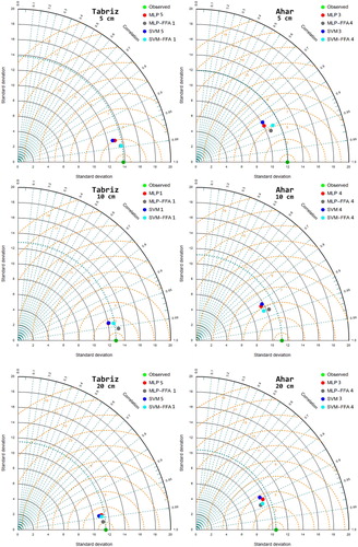
Figure 9. Taylor diagrams (with a delay of two days).

As it is clear by an overabundance of statistical parameters and graphical evaluation, it is convincing that the accuracy of the MLP-FFA and SVM-FFA models far surpasses the non-optimized models. Therefore, FFA certifies that the hybrid model can avoid any premature convergence of process, which is likely to maximize the ability of the hybrid MLP-FFA and SVM-FFA models. According to statistical and graphical evaluations, MLP-FFA and SVM-FFA were found to be a sufficient tool for predicting soil temperature values using meteorological parameters as the inputs and can be used as practical models with a high degree of applicability for ST estimation.

Sensitivity analysis

For investigating the influence of input parameters on the ST prediction, the RMSE and R² evaluation criteria utilized for different groupings of input variables. For this purpose, the SVM model in predicting ST_10cm with a delay of one and two days selected for sensitivity analysis (Tables 7 and 8). Each model confirmed the extents to which the eliminated variable would affect the model accuracy. As it is clear from Tables 7 and 8, the precision of the SVM model decreased if each of T, RH, SUN, and W input parameters removed in the modeling. Furthermore, it comprehended that T has the most significant effect in increasing the prediction accuracy. In other words, eliminating T caused a sharp increase in RMSE value in all studied conditions.

Table 7. Effect of removing input variables on the SVM model accuracy for predicting ST_10cm for Tabriz and Ahar stations with a delay of one day

		Tabriz		Ahar
Model	Input parameters	R^2	RMSE (°C)	R^2	RMSE (°C)
1	All	0.94	2.56	0.76	5.75
2	Remove T	0.71	6.15	0.43	8.65
3	Remove SUN	0.94	2.57	0.73	6.16
4	Remove RH	0.94	2.59	0.76	5.83
5	Remove W	0.93	2.58	0.76	5.83

Table 8. Effect of removing input variables on the SVM model accuracy for predicting ST_10cm for Tabriz and Ahar stations with a delay of two days.

		Tabriz		Ahar
Model	Input parameters	R^2	RMSE (°C)	R^2	RMSE (°C)
1	All	0.95	2.64	0.75	5.89
2	Remove T	0.71	6.17	0.42	8.70
3	Remove SUN	0.94	2.72	0.72	6.33
4	Remove RH	0.94	2.70	0.74	5.95
5	Remove W	0.94	2.65	0.74	5.94

Additionally, as the limitations of the current study, it should be noted that the used dataset was related to two Tabriz and Ahar stations, Iran. Therefore, the mentioned stations have approximately similar climates. Thus, it would have been better if extra stations with different environments were tested for examining the accuracy of implemented methods.

Conclusions

Soil temperature as one of the main characteristics of the soil affects many aspects of life, especially the distribution of plants, animals, biological activities, and water movement in the soil. Furthermore, soil temperatures are useful in cases such as the length of growth, the spread of plant diseases, the readability of the soil water, the growth and development of roots. The determination of models that can accurately estimate the temperature of different soil levels is essential for agricultural research. In the present research, we tried to estimate ST values at various depths of 5, 10, and 20 cm using the MLP, SVM, and their hybrid version with a firefly optimization algorithm (MLP-FFA and SVM-FFA). The meteorological parameters of Tabriz station have been gathered, and five diverse groups were prepared with one and two days delay. The results attained exposed that in the case of using one day delay for the depths of 5, 10 and 20 cm, the most precise models were SVVM-FFA1, MLP-FFA1, MLP-FFA5 (with RMSE values of 2.15°C, 1.58°C, and 1.17°C) at Tabriz station and MLP-FFA3, MLP-FFA4, MLP-FFA3 (with RMSE values of 4.64°C, 4.51°C and 3.95°C) at Ahar station, respectively. Additionally, in the case of using two days delay for the depths of 5, 10 and 20 cm, the most precise models were MLP-FFA4, SVM-FFA4, MLP-FFA3 (with RMSE values of 1.71°C, 1.63°C and 1.15°C) at Tabriz station and SVM-FFA4, MLP-FFA1, SVM-FFA4 (with RMSE values of 4.60°C, 4.47°C, and 3.69°C) at Ahar station, respectively. Moreover, it can be comprehended from obtained results that the hybrid models of FFA (i.e. MLP-FFA and SVM-FFA) produced a substantial decrease in error metrics compared to the standalone MLP and SVM models. In conclusion, the acquired results endorsed the adequacy of the hybrid MLP-FFA and SVM-FFA models and pointed out the efficiency of the FFA algorithm for soil temperature estimations. Future work can be done for examining the effects of different optimization algorithms on the accuracy of MLP and SVM models for ST estimation at different climates.

Acknowledgment

We aknowledge the ‘Open Access Funding by the Publication Fund of the TU Dresden’. The support of the German Research Foundation and the Bauhaus-Universität Weimar is also aknowledged.

Disclosure statement

No potential conflict of interest was reported by the author(s).

Additional information

Funding

This work was supported by European Commission: [Grant Number 2017-1.3.1-VKE-2017-00025,EFOP-3.6.1-16-2016-00010].

References

- Beltrami, H. (2001). On the relationship between ground temperature histories and meteorological records: A report on the Pomquet station. Global and Planetary Change, 29(3-4), 327–348. https://doi.org/10.1016/S0921-8181(01)00098-4
- Bilgili, M. (2010). Prediction of soil temperature using regression and artificial neural network models. Meteorology and Atmospheric Physics, 110(1–2), 59–70. https://doi.org/10.1007/s00703-010-0104-x
- Bilgili, M. (2011). The use of artificial neural networks for forecasting the monthly mean soil temperatures in Adana, Turkey. Turkish Journal of Agriculture and Forestry, 35(1), 83–93. doi:10.3906/tar-1001-593.
- Burges, C. J. C. (1998). A tutorial on support vector machines for pattern recognition. Data Mining and Knowledge Discovery, 2(2), 121–167. https://doi.org/10.1023/A:1009715923555
- Chau, K. W., & Muttil, N. (2007). Data mining and multivariate statistical analysis for ecological system in coastal waters. Journal of Hydroinformatics, 9(4), 305–317. https://doi.org/10.2166/hydro.2007.003
- Cheng, C. T., Lin, J. Y., Sun, Y. G., & Chau, K. W. (2005). Long-term prediction of discharges in Manwan Hydropower using adaptive-network-based fuzzy inference systems models. Lecture Notes in Computer Science, 3612, 1152–1161. https://doi.org/10.1007/11539902_145
- Citakoglu, H. (2017). Comparison of artificial intelligence techniques for prediction of soil temperatures in Turkey. Theoretical and Applied Climatology, 130(1-2), 545–556. https://doi.org/10.1007/s00704-016-1914-7
- Deo, R. C., & Sahin, M. (2015). Application of the Artificial neural network model for prediction of monthly standardized precipitation and evapotranspiration index using hydrometeorological parameters and climate indices in eastern Australia. Atmospheric Research, 161–162, 65–81. https://doi.org/10.1016/j.atmosres.2015.03.018
- Deo, R. C., & Sahin, M. (2017). Forecasting long-term global solar radiation with an ANN algorithm coupled with satellite-derived (MODIS) land surface temperature (LST) for regional locations in Queensland. Renewable and Sustainable Energy Reviews, 72, 828–848. https://doi.org/10.1016/j.rser.2017.01.114
- Firat, M., & Gungor, M. (2009). Generalized regression neural networks and feed forward neural networks for prediction of scour depth around bridge piers. Advances in Engineering Software, 40(8), 731–737. https://doi.org/10.1016/j.advengsoft.2008.12.001
- Fister, I., Fister Jr., I., Yang, I. X. S., & Brest, J. (2013). A comprehensive review of firefly algorithms. Swarm and Evolutionary Computation, 13, 34–46. https://doi.org/10.1016/j.swevo.2013.06.001
- Fotovatikhah, F., Herrera, M., Shamshirband, S., Chau, K. W., Faizollahzadeh Ardabili, S., & Piran, J. (2018). Survey of computational intelligence as basis to big flood management: Challenges, research directions and future work. Engineering Applications of Computational Fluid Mechanics, 12(1), 411–437. https://doi.org/10.1080/19942060.2018.1448896
- Gazi, V., & Passino, K. M. (2004). Stability analysis of social foraging swarms. IEEE Transactions on Systems, Man and Cybernetics, Part B (Cybernetics), 34(1), 539–557. https://doi.org/10.1109/TSMCB.2003.817077
- Ghorbani, M. A., Ahmadzadeh, H., Isazadeh, M., & Terzi, O. (2016). A comparative study of artificial neural network (MLP, RBF) and support vector machine models for river flow prediction. Environmental Earth Sciences, 75(6), 476–490. https://doi.org/10.1007/s12665-015-5096-x
- Ghorbani, M. A., Shamshirband, S., Zare Haghi, D., Azani, A., Bonakdari, H., & Ebtehaj, I. (2017). Application of firefly algorithm-based support vector machines for prediction of field capacity and permanent wilting point. Soil and Tillage Research, 172, 32–38. https://doi.org/10.1016/j.still.2017.04.009
- Gill, M. K., Asefa, T., Kemblowski, M. W., & McKee, M. (2006). Soil moisture prediction using support vector machines. Journal of the American Water Resources Association, 42(4), 1033–1046. https://doi.org/10.1111/j.1752-1688.2006.tb04512.x
- Gleckler, P. J., Taylor, K. E., & Doutriaux, C. (2008). Performance metrics for climate models. Journal of Geophysical Research, 113(D6), 1–20. https://doi.org/10.1029/2007JD008972
- Hanks, R. J., Austin, D. D., & Ondrechan, W. T. (1971). Soil temperature estimation by a numerical method. Proceedings Soil Science Society of America, 35, 665–667. doi:10.2136/sssaj1971.03615995003500050015x.
- Hillel, D. (1998). Environmental soil physics (p. 771). Academic Press.
- Kazemi, S. M. R., Minaei Bidgoli, B., Shamshirband, S., Karimi, S. M., Ghorbani, M. A., Chau, K. W., & Kazem Pour, R. (2018). Novel genetic-based negative correlation learning for estimating soil temperature. Engineering Applications of Computational Fluid Mechanics, 12(1), 506–516. https://doi.org/10.1080/19942060.2018.1463871
- Kim, S., & Singh, V. P. (2014). Modeling daily soil temperature using data-driven models and spatial distribution. Theoretical and Applied Climatology, 118(3), 465–479. https://doi.org/10.1007/s00704-013-1065-z
- Kisi, O., Tombul, M., & Kermani, M. Z. (2015). Modeling soil temperatures at different depths by using three different neural computing techniques. Theoretical and Applied Climatology, 121(1-2), 377–387. https://doi.org/10.1007/s00704-014-1232-x
- Kurup, P. U., & Dudani, N. K. (2002). Neural networks for profiling stress history of clays from PCPT data. Journal of Geotechnical and Geoenvironmental Engineering, 128(7), 569–579. https://doi.org/10.1061/(ASCE)1090-0241(2002)128:7(569)
- Mazou, E., Alvertos, N., & Tsiros, I. X. (2013). Soil temperature prediction using time-delay neural networks. Advances in Meteorology, Climatology and Atmospheric Physics, 611–615. https://doi.org/10.1007/978-3-642-29172-2_87
- McClelland, J., & Rumelhart, D. (1988). Explorations in parallel distributed processing: A handbook of models, programs, and exercises. MIT Press.
- Mehdizadeh, M., Behmanesh, J., & Khalili, K. (2018). Comprehensive modeling of monthly mean soil temperature using multivariate adaptive regression splines and support vector machine. Theoretical and Applied Climatology, 133(3-4), 911–924. https://doi.org/10.1007/s00704-017-2227-1
- Moazenzadeh, R., Mohammadi, B., Shamshirband, S., & Chau, K. W. (2018). Coupling a firefly algorithm with support vector regression to predict evaporation in northern Iran. Engineering Applications of Computational Fluid Mechanics, 12(1), 584–597. https://doi.org/10.1080/19942060.2018.1482476
- Pal, M. (2006). Support vector machines-based modelling of seismic liquefaction potential. International Journal for Numerical and Analytical Methods in Geomechanics, 30(10), 983–996. https://doi.org/10.1002/nag.509
- Plauborg, F. (2002). Simple model for 10 cm soil temperature in different soils with short grass. European Journal of Agronomy, 17(3), 173–179. https://doi.org/10.1016/S1161-0301(02)00006-0
- Qasem, S. N., Samadianfard, S., Kheshtgar, S., Jarhan, S., Kisi, O., Shamshirband, S., & Chau, K. W. (2019). Modeling monthly pan evaporation using wavelet support vector regression and wavelet artificial neural networks in arid and humid climates. Engineering Applications of Computational Fluid Mechanics, 13(1), 177–187. https://doi.org/10.1080/19942060.2018.1564702
- Qian, B., Gregorich, E. G., Gameda, S., Hopkins, D. W., & Wang, X. L. (2011). Observed soil temperature trends associated with climate change in Canada. Journal of Geophysical Research, 116(D2), 1–16. https://doi.org/10.1029/2010JD015012
- Sabziparvar, A. A., Tabari, H., & Aeini, A. (2010). Estimation of mean daily soil temperature by means of meteorological data in some selected climates of Iran. Water And Soil Science (Journal Of Science and Technology of Agriculture and Natural Resources), 14(52), 125–137. (In Persian). http://jstnar.iut.ac.ir/article-1-1229-en.html.
- Sabziparvar, A. A., Zare Abyaneh, H., & Bayat Varkeshi, M. (2010). A model comparison between predicted soil temperatures using ANFIS model and regression methods in three different climates. Journal of Water and Soil (Agricultural Sciences and Technology), 24(2), 274–285. (In Persian). https://www.sid.ir/en/journal/ViewPaper.aspx?ID=177202.
- Samadianfard, S., Asadi, E., Jarhan, S., Kazemi, H., Kheshtgar, S., Kisi, O., Sajjadi, S., & Abdul Manaf, A. (2018). Wavelet neural networks and gene expression programming models to predict short-term soil temperature at different depths. Soil and Tillage Research, 175, 37–50. https://doi.org/10.1016/j.still.2017.08.012
- Samadianfard, S., Delirhasannia, R., Kisi, O., & Agirre-Basurko, E. (2013). Comparative analysis of ozone level prediction models using gene expression programming and multiple linear regression. Geofizika, 30(1), 43–74. https://hrcak.srce.hr/105853.
- Samadianfard, S., Ghorbani, M. A., & Mohammadi, B. (2018). Forecasting soil temperature at multiple-depth with a hybrid artificial neural network model coupled-hybrid firefly optimizer algorithm. Information Processing in Agriculture, 5, 465–476. https://doi.org/10.1016/j.inpa.2018.06.005
- Samadianfard, S., Majnooni-Heris, A., Qasem, S. N., Kisi, O., Shamshirband, S., & Chau, K. W. (2019). Daily global solar radiation modeling using data-driven techniques and empirical equations in a semi-arid climate. Engineering Applications of Computational Fluid Mechanics, 13(1), 142–157. https://doi.org/10.1080/19942060.2018.1560364
- Samadianfard, S., Sattari, M. T., Kisi, O., & Kazemi, H. (2014). Determining flow friction factor in irrigation pipes using data mining and artificial intelligence approaches. Applied Artificial Intelligence, 28(8), 793–813. https://doi.org/10.1080/08839514.2014.952923
- Sanikhani, H., Deo, R. C., Yaseen, Z. M., Eray, O., & Kisi, O. (2018). Non-tuned data intelligent model for soil temperature estimation: A new approach. Geoderma, 330, 52–64. https://doi.org/10.1016/j.geoderma.2018.05.030
- Sihag, P., Esmaeilbeiki, F., Singh, B., & MuhammedPandhiani, S. (2019). Model-based soil temperature estimation using climatic parameters: The case of Azerbaijan province, Iran. Geology, Ecology, and Landscapes. https://doi.org/10.1080/24749508.2019.1610841
- Tabari, H., Sabziparvar, A. A., & Ahmadi, M. (2011). Comparison of artificial neural network and multivariate linear regression methods for estimation of daily soil temperature in an arid region. Meteorology and Atmospheric Physics, 110(3–4), 135–142. https://doi.org/10.1007/s00703-010-0110-z
- Tabari, H., Talaee, P. H., & Willems, P. (2015). Short-term forecasting of soil temperature using artificial neural network. Meteorological Applications, 22(3), 576–585. https://doi.org/10.1002/met.1489
- Taylor, K. E. (2001). Summarizing multiple aspects of model performance in a single diagram. Journal of Geophysical Research: Atmospheres, 106(D7), 7183–7192. https://doi.org/10.1029/2000JD900719
- Ustaoglu, B., Cigizoglu, H. K., & Karaca, M. (2008). Forecast of daily mean, maximum and minimum temperature time series by three artificial neural network methods. Meteorological Applications, 15(4), 431–445. https://doi.org/10.1002/met.83
- Vapnik, V. N. (1995). The nature of statistical learning theory. Springer-Verlag. ISBN 0-387-98780-0.
- Wu, W., Tang, X. P., Guo, N. J., Yang, C., Liu, H. B., & Shang, Y. F. (2013). Spatiotemporal modeling of monthly soil temperature using artificial neural networks. Theoretical and Applied Climatology, 113(3-4), 481–494. https://doi.org/10.1007/s00704-012-0807-7
- Yang, X. S. (2008). Introduction to mathematical optimization. In From linear programming to metaheuristics. Cambridge, UK: Cambridge International Science Publishing. ISBN 978-1-904602-82-8. https://www.waterstones.com/book/introduction-to-mathematical-optimization/xin-she-yang/9781904602828.
- Yaseen, Z. M., Sulaiman, S. O., Deo, R. C., & Chau, K. W. (2019). An enhanced extreme learning machine model for river flow forecasting: State-of-the-art, practical applications in water resource engineering area and future research direction. Journal of Hydrology, 569, 387–408. https://doi.org/10.1016/j.jhydrol.2018.11.069
- Zheng, D., Hunt Jr., E. R., & Running, S. W. (1993). A daily soil temperature model based on air temperature and precipitation for continental applications. Climate Research, 2(3), 183–191. https://doi.org/10.3354/cr002183