Simulation and experimental study of influences of shape of roller on the lubrication performance of precision speed reducer

Abstract

This paper presents a study to investigate the effects of the shape of rollers in high precision enveloping speed reducer on the reducer’s lubrication performance. Theoretical models for the precision speed reducer with cylindrical and conical rollers as its transmission components were constructed at first based on the meshing theory. Next, numerical analysis was conducted investigate the lubrication status of the speed reducers with different types of rollers at four rotation speeds using ParticleWorks. The moving particle semi-implicit method embedded in that software was used to model the reducers and the inside lubricant flow. A sequence of tests was performed to inspect the transmission efficiency of the reducers at four different rotation speeds. Experimental data were compared to the simulation predictions. Comparisons showed that the data measured from the experiments matched the simulation results very well. Both experimental and computational results confirmed that the lubrication performance of the enveloping speed reducer with conical rollers is better than that of the speed reducer with cylindrical rollers. It has also been proven that the method of using the churning power losses to assess the effects of the shape of the rollers on the roller enveloping speed reducer’s lubrication behavior is highly reliable.

KEYWORDS:

• Lubrication performance
• churning power loss
• precision speed reducer
• cylindrical roller
• conical roller
• computational fluid dynamics (CFD)

1. Introduction

Modern industry (high-end CNC equipment, industrial robots, radar, etc.) places higher requirements on high precision transmission devices. The desired transmission devices should not only have a compact size, large gear ratio, and high precision of transmission, but should also provide enhanced transmission efficiency, improved load bearing capacity, and enable the smooth transmission. The latter capabilities are directly related to lubrication performance of those devices. The higher lubrication performance a transmission device has, the higher transmission efficiency it can attain with a longer life expectancy and at a reduced noise level. However, most of the currently used transmission devices employ gear pairs that incorporate sliding friction. The sliding friction between the mating teeth in contact leads to considerable dynamic effects, causes noise and power losses, and seriously reduces the performance of the transmission device.

In order to eliminate the detrimental effects caused by the sliding friction, many researchers tried to replace the sliding friction with rolling friction in gear transmission design. Motohashi et al. (1986) presented a transmission system for the first time. The transmission system consisted of a pair of a globoidal cam and its mating roller wheel. The unique gear meshing featured in their design could effectively reduce backlash, enhance the lubrication performance, and therefore has attracted large amounts of interest and attention (Simon, 2008; Zhong & Yang, 2015). Enlightened by Motohashi’s and other previous studies, Deng et al. (2019a, 2019b, 2019c, 2019d) invented two roller enveloping hourglass worm gear sets with high precision. In the developed worm gear sets, the traditional sliding friction was replaced by the rolling friction to significantly reduce the meshing friction and acquire higher transmission efficiency.

Deng et al. (2012) conducted a theoretical analysis in an effort to reveal how different roller shapes (cylindrical roller, conical roller, and spherical roller) affect the lubrication performance. However, the employed theoretical approach has never been validated through experiments; therefore, the reliability of using that theoretical method for design optimization of parameters of the worm gear set cannot be ensured. Thus, it is imperative to find a reliable method with a set of indicators for evaluation and assessment of the lubrication behavior of high precision roller enveloping speed reducers.

Three methods that have long been used for such studies are: experimental method, numerical simulation method, and combined experimental-computational method. Among the previous experimental studies, Chen and Matsumoto (2016) clarified the effect of the relative position between gears and the shape of the casing wall of the gearbox on the oil churning losses and confirmed that besides the common factors (relative position, casing wall shape, etc.), the level of lubricant also significantly affects the churning losses. Laruelle et al. (2017) carried out a sequence of experiments on single bevel gears partially submerged in oil to discover the effects of viscosity of lubricant, gear speed and geometry, and temperature on the splash power losses. According to the experimental data, they developed an extended formula to calculate the churning losses of those bevel gears. Leprince et al. (2012) established a test rig for spur gears to determine the amount of lubricant scattered at different places on the casing walls and constructed a sequence of equations on the basis of the measured data to estimate the lubricant projected by the spur gears rotating in an oil bath. The experimental method is suitable for analysis of low-to-medium speed gears but such method can be very costly for the dynamic analysis of high speed gears because the required test rig and auxiliary facilities are very expensive. In addition, because of the constraints of the current experimental technology, it is still very hard to monitor the instantaneous speed of splashing lubricant and the distribution of the lubricant within the speed reducer.

Compared with the experimental method, the simulation method is an effective tool allowing quantitative analysis of high-speed gears in a time- and cost-effective manner. For example, Liu et al. (2018) established a computational model for a dip-lubricated planetary test gearbox and employed the model to acquire a graphical depiction of distribution of lubricant within the gearbox via computational analysis. Concli and Gorla (2017) suggested a new automated mesh-partitioning method and applied that method for CFD simulation of a planetary gearbox and obtained its churning losses. Renjith et al. (2015) focused on the factors that influence the churning loss of the automobile differential system and formulated a mathematical model for estimating the spin power loss of that system and validated that model via CFD simulation. Most recently, Salih et al. (2019) developed an adaptive mesh refinement (AMR) algorithm integrated with the cut-cell immersed boundary method (IBM) for solving thin-object fluid interaction simulation problems. The developed AMR-IBM algorithm was verified using a benchmark data of fluid passing through a cylinder and the results showed that there was a good agreement under laminar flow. The accuracy and reliability of the developed algorithm in predicting flow characteristics in the boundary layers of thin structures were confirmed through simulations. Ghalandari et al. (2019) employed the boundary element method (BEM) – finite element method (FEM) to investigate the sloshing and flexibility terms of elastic submerged structures on the behavior of a coupled domain. A code was developed based on the BEM-FEM model to be used for solving an arbitrary 2D and 3D tank with an irregularly shaped elastic submerged structure. The numerical results were compared against the data published in previous papers and the deviations were within 2%. The above simulation analyses followed a computational approach, which is much less expensive than the experimental approach, and the results can be easily accessed and observed. However, such method highly depends on the capacity of computing facilities and the reliability of simulation software, and the results are very sensitive to boundary conditions. Therefore, the results obtained from the numerical simulations must be verified and validated.

A combined experimental-computational approach can take maximal advantages of both experimental and computational methods’ benefits while overcoming the limitations of each method. Applying this approach to the study of the lubrication performance within a gear system, a regular process is to verify and validate the computational simulation method via experiments in the early stage and then use the validated computational method for analysis in the latter stages. Through this process, the computational and experimental methods can complement each other to maximally reduce research costs while acquiring accurate results. For instance, Hu et al. (2019) validated the accuracy and efficiency of using the CFD method to predict the churning losses of spiral bevel gears by conducting experiments on the losses of such gears at first, and then used the CFD method to analyze the effects of rotation speed, level, temperature, density, and dynamic viscosity of the lubricant, as well as the tilt angle on the churning power losses. Ji et al. (2018) used CFD simulation to analyze physical characteristics of oil in rotating spur gears, such as the number and size of bubbles created by the rotating gears, the velocity profile and velocity field below the lubricant level, etc. The simulation data were compared to the results measured from a digital particle image velocimetry and a comparatively good agreement was found. Jiang et al. (2019) also applied a integrated computational-experimental approach to study the effect of an oil guide device on lubrication performance of spiral bevel geared transmissions. Akbarian et al. (2018) conducted experimental and CFD-based numerical simulations on a dual-fueled constant speed engine to characterize the emissions and performance of a diesel engine subjects to different loads and pilot to gaseous fuel ratios. The CFD results showed good agreements with the results measured from the experiments.

Unlike the transmission systems researched in the studies mentioned above, the core component of roller enveloping speed reducers is worm, which has complicated spatial curved surfaces that require an advanced mesh generation strategy in a computational environment. Meanwhile, since an enveloping speed reducer consists of many rollers, it is therefore imperative to understand how the individual rollers impact the lubrication performance of such a device.

In the present study, we employ the integrated computational-experimental approach to investigate the lubrication behavior of the enveloping worm face reducer with cylindrical rollers. This work features the application of the MPS method in modeling and analysis of worm gear drives that involve complicated tooth surfaces. Also, to the best of our knowledge, the present simulation work for the first time considers the churning power losses caused by bearings. In experimental analysis, instead of measuring the churning losses, we recorded transmission efficiency of the speed reducer and used it to validate the employed MPS method and CFD simulations. This is because the power losses measured from experiments also include the friction losses and cannot properly represent the power losses due to oil churning.

The rest of the paper is structured as follows. Section 2 introduces meshing characteristics of the roller enveloping worm transmission and provides theoretical analyses of its lubrication performance. Section 3 describes experimental and computational investigations of such a transmission system. Findings from those studies are discussed in Section 4, and the paper is closed by the conclusion section, Section 5.

2. Theoretical analysis

One main difference between the roller enveloping hourglass worm and traditional worms is that the sliding friction becomes the rolling friction with the application of rollers. Therefore, the enveloping worm face speed reducer offers many advantages including high efficiency, low noise, high speed ratio, and long-life expectancy.

2.1. Lubrication angle

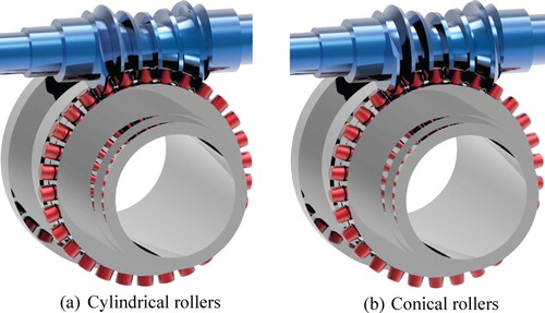
As shown in Figure 1, roller enveloping speed reducers transmit power through the meshing between the rollers of the worm and the worm gear. Commonly used rollers include cylindrical, conical, and spherical rollers. Since the special equipment for fabricating the speed reducer with spherical balls has yet to be developed, in this study, we only discuss the influences of cylindrical and conical rollers on the roller enveloping reducers’ lubrication performance via experimental verification.

Figure 1. Roller enveloping worm face speed reducers with different types of rollers. (a) cylindrical rollers; (b) conical rollers.

According to the gear meshing theory, relative velocity between the worm gear and the worm at the contact point should satisfy the equation as follows: v¹²·n = 0. Here v¹² is the relative velocity vector at the contact point, and n is the unit normal vector at that point.

As derived by Deng et al. (2019c, 2019d), the meshing equations for the worm gear set are (1) $\{\begin{array}{l}{\mathit{v}}^{12}\cdot \mathit{n}=M_1\cos {\phi }_2-M_2\sin {\phi }_2-M_3=0\\ \begin{array}{l}{M}_1=(c_2+x_0)\sin \alpha \sin \theta \\ +(a_2-y_0\sin \alpha -z_0\cos \alpha )\cos \theta \end{array}\\ \begin{array}{l}{M}_2=-(c_2+x_0)\cos \alpha \sin \theta \\ +(b_2+y_0\cos \alpha -z_0\sin \alpha )\cos \theta \end{array}\\ M_3=i_{21}(b_2+y_0\cos \alpha -z_0\sin \alpha )\sin \alpha \sin \theta \\ +i_{21}(a_2-y_0\sin \alpha -z_0\cos \alpha )\cos \alpha \sin \theta +A\cos \theta \end{array}$(1) where M₁, M₂, and M₃ are coefficients; x₀, y₀, and z₀ locate the coordinate of the contact point; and i₂₁ represents the gear ratio. For cylindrical rollers, x₀= Rcosθ, y₀= Rsinθ, z₀= u; for conical rollers, x₀= usinβcosθ, y₀= usinβsinθ, z₀= ucosβ; where u, θ, R, β are design parameters of the rollers. ϕ₂ denotes the angle of rotation of the worm gear.

The lubrication angle is the angular separation between the relative velocity and the contact curve and is employed to assess the lubrication conditions between two conjugated surfaces (Litvin & Fuentes, 2004; Deng et al., 2012). A relatively large lubrication angle will facilitate the creation of a hydrodynamic oil film in an arc-surface worm drive. Therefore, the closer that angle is to 90°, the better lubrication performance the worm drive will attain. As proposed by Deng et al. (2012), the lubrication angle of a worm gear set (μ), which is an acute angle, can be calculated as (2) $\mu =\arcsin \frac{|v_1^{12}((v_1^{12}/R)-{\omega }_2^{12})+v_2^{12}{\omega }_1^{12}|}{\begin{array}{c}\sqrt{{((v_1^{12}/R)-{\omega }_2^{12})}^2+{({\omega }_1^{12})}^2}\\ \sqrt{{(v_1^{12})}^2+{(v_2^{12})}^2}\end{array}}$(2) In above equation, R denotes the roller radius; v¹² and ω¹² are relative linear and angular velocity, respectively. Subscript ‘1’ indicates the worm (driving part) and ‘2’ indicates the worm gear (driven part).

Key design parameters for the two types of rollers are listed in Table 1. The parametric values were obtained by Deng et al. (2019a) via a combined theoretical, computational, and experimental analysis. Using those values and based on Equation (2), we calculate the lubrication angle when the rotational angle ϕ₂ varies between −30° and 30°. Figure 2 compares the lubrication angle yielded from the cylindrical and conical rollers. From that figure, it can be seen that the lubrication angles for both types of rollers reach their maxima at the beginning and the ending position of engagement, which means that the optimal lubrication performance would be acquired at those moments. Throughout the entire process, the lubrication angle curve of the conical rollers shows less variation, which indicates a better lubrication performance.

Figure 2. Lubrication angles for cylindrical and conical rollers.

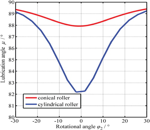
Table 1. Key design parameters.

Parameters	Center distance A	Transmission ratio i12	Roller radius R
Cylindrical roller	80 mm	30	5 mm
Conical roller	80 mm	30	5 mm

2.2. Computational method

The authors had tried to use ANSYS Fluent, a powerful CFD software to mesh the computational model of the speed reducers and their internal lubricant flow. However, the quality of the meshes at ending surfaces of the worm was very poor and the distortion of individual elements in those areas reached 0.9. Even worse, more poor-quality meshes were generated during the simulation because of high relative velocity between the surfaces of the worm and worm gear, which led to negative volumes and caused abrupt terminations of the simulation. Therefore, such problem can only be solved using meshfree methods such as particle methods.

The moving particle semi-implicit (MPS) method is applied for numerical simulations. As a meshfree method, the MPS method can effectively eliminate the error caused by tangled meshes and remeshing when the material being simulated moves around the device. Such a method is especially suitable for simulating incompressible flows and calculating flow fields. Deng et al. have used the MPS method to study the lubrication conditions in the gear transmission system of a high-speed railway train (2020a) and the internal flow field of a worm gear drive (2020b). Li et al. (2018) also successfully employed this method to compute the churning losses of a single helical gear in a gear system. The computational data were quite close to the data measured from experiments.

The MPS method was put forward by Koshizuka et al. in 1995. It is a meshfree particle method for solving incompressible free surface flow. In that method, the incompressible Navier-Stokes equation is discretized with a Taylor series. Its governing equations include the incompressible Navier-Stokes equation and an equation of continuity, as expressed in Equations (3) and (4)

Navier-Stokes equation (law of momentum conservation) (3) $\frac{Du}{Dt}=-\frac{\mathrm{\nabla }P}{\rho }+\nu {\mathrm{\nabla }}^{2}u+g$(3)

Equation of continuity (law of mass conservation) (4) $\frac{D\rho }{Dt}=0$(4) where u denotes the velocity, P is the pressure, ρ represents the density, ν denotes the kinetic viscosity, g is the gravity, and $(D/Dt)$ denotes the Lagrangian time derivative.

In the MPS method, the Navier-Stokes equation is solved following two steps: implicit calculation and explicit calculation. The pressure term is calculated in the implicit step and all other terms are calculated in the explicit step using the Laplacian model.

The pressure term is implicitly calculated using (5) ${\mathrm{\nabla }}^2{p}^{n+1}=\frac{\rho }{\mathrm{\Delta }{t}^2}\frac{n^{\ast }-n^0}{n^0}$(5)

Other terms are explicitly calculated using (6) $\frac{u^{\ast }-u^k}{\mathrm{\Delta }t}=\nu {\mathrm{\nabla }}^2{u}^k+g$(6)

A correction step is needed to rectify velocity and position based on the pressure gradient (7) $\frac{u^{k+1}-u^{\ast }}{\mathrm{\Delta }t}=-\frac{\mathrm{\nabla }{P}^{k+1}}{\rho }$(7) n and n⁰ in Equation (5) represent the density of the particle number and its initial value, respectively; superscript ‘k’ in Equations (6) and (7) indicates timestep; and superscript ‘*’ in above equations denotes a physical quantity after completing the explicit calculation.

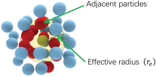
In the MPS method, a particle interacts with close-by particles in an area defined by a kernel function proposed by Koshizuka and Oka (1996) (Equation (8)). If the interparticle distance is greater than the radius of that area, the kernel function will be 0. That radius is known as the effective radius and all the particles inside the effective radius are close-by particles (Figure 3). The effective radius (r_e) of a particle is set as two to four times of the diameter of that particle so as to maintain a constant number of particles within the effective radius. (8) $w(r_{ij})=\{\begin{array}{ll}{\displaystyle \frac{r_e}{r_{ij}}}-1& (r_{ij}\le r_e)\\ 0& (r_{ij}>r_e)\end{array}$(8)

Figure 3. Neighboring particles (red) around the particle (olive green) inside r_e.

In Equation (8), i and j refer to particle numbers, r_ij is the distance between particle i and j (r_ij = |r_i − r_j|), and r represents the particle position vector.

The number density of particles at the location of particle i is defined as the summation of the kernel functions, which is $n_i={\sum }_{j\ne i}w(r_{ij})$. It should be noted that r_ij is calculated by the computer program and the MPS method does not use reference volume to determine the particle number density n_i.

The inter-particle collision force that individual particles subject to is decomposed into a normal (F_n), a shear (tangential) (F_s), and a damping component (F_d) as F = F_n + F_s + F_d. Figure 4 shows the collision force generated due to the impact between particles. A flowchart of the MPS-based simulation is displayed in Figure 5.

Figure 4. Schematic showing the interparticle forces.

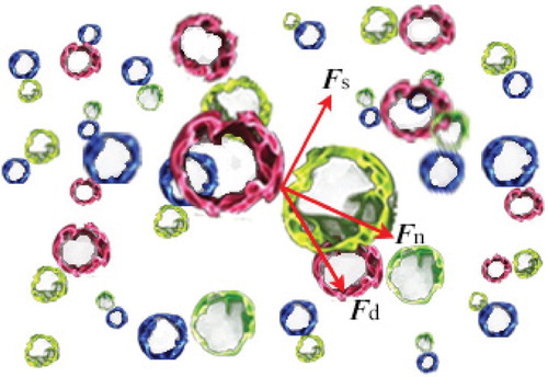
Figure 5. Diagram of MPS simulation steps.

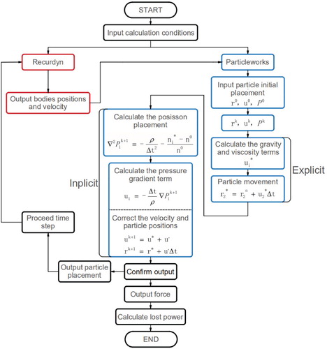
Churning losses of a rotating part can be determined from its churning loss torque as P_j = |T_j|n_j/9550, where n_j is the part’s speed and T_j the churning loss torque is computed by adding external torques of all particles together. The overall churning loss is then obtained by adding together the losses of each rotating part as $P={\sum }_{j=1}^k(|T_j|n_j/9550)$, where k is the total number of the rotating parts in the system. For more details on calculating the churning losses and churning loss torque, please refer to Deng et al. (2020b).

3. Numerical analysis

3.1. Computational model

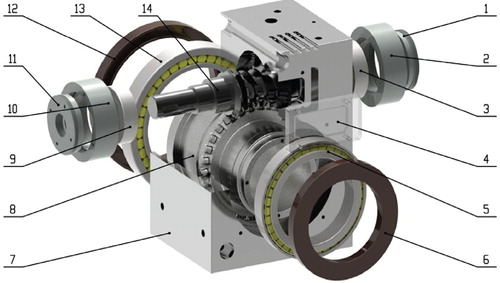
Faithful 3D CAD models for the enveloping speed reducers were created and validated following the approach presented by Deng et al. (2019a, 2012) (Figure 6). In creating the initial detailed 3D models, two speed reducers with cylindrical and conical rollers, which were prototyped for experimental analysis, were scanned using a Romer Absolute Arm 3D Coordinate Measuring Machine (CMM) equipped with Geomagic 3D software. The scanned data was read into a computer to create detailed three-dimensional models. With the aim of enhancing the efficiency while preserving the accuracy of the simulation, chamfers and position holes outside the casing were removed from the high-fidelity models while all features inside the casing were kept.

Figure 6. Layout of parts in the enveloping speed reducer: (1) right end cover; (2) right shaft bushing; (3) right worm shaft bearing; (4) observation window; (5) front worm gear bearing; (6) front seal ring; (7) casing; (8) worm gear; (9) left worm shaft bearing; (10) left shaft bushing; (11) left end cover; (12) rear seal ring; (13) rear worm gear bearing; (14) worm.

3.2. Numerical simulation

A MPS-based CFD software, Particleworks, was used for the CFD simulations. Particleworks is the leading software for simulating fluid flows in complicated geometries, e.g. free surface flow inclusive of splash, and gear lubricant behavior. It uses the geometry directly imported from CAD models and proceeds to analyze condition settings and calculations without mesh generation. The effectiveness and accuracy of this software have been verified in many previous and recent studies (Khayyer & Gotoh, 2009; Sakai et al., 2012; Duan et al., 2017, 2019).

The simplified models were then imported into Particleworks, and dynamic parameters are defined and assigned to the models. The entire simulation time is set as five seconds to minimize the influence of abrupt change of rotation speed on the computational results. During the simulation, an acceleration stage (from 0 to 0.5 s) was defined to simulate the starting of this speed reducer, which was followed by a uniform rotation period from 0.5 to 5 s. The application phase was introduced to alleviate the effect of sudden changes of rotation speed on the condition of the fluid. Velocities of each component were then defined. To simplify the calculations, we only considered the speed of revolution of cages and bearings while ignoring the rotation of individual rollers.

Next, fluid parameters were set in ParticleWorks. The simplified components of the speed reducer were drawn as polygons, and the lubricant was modeled as a fluid, which is a group of particles. Due to the maximum computing capacity, the diameter of each lubricant particle was set as 2 mm, and an air density at an ambient temperature of 40°C and at sea level (1.097 kg/m³) were applied in this calculation. According to the design standards of the speed reducer, lubricant and oil depth must be selected based on the worm parameters. In this study, the viscosity and density of the lubricant are 100 cst and 850 kg/m³, respectively; and one-third of the height of the worm gear is immersed in oil.

In addition, it is critical to determine a proper initial timestep for simulating the liquid flow using ParticleWorks software (Prometech Software, 2016). The timestep should be less than a threshold value to ensure the convergence of the calculation while a timestep too small will result in a unnecessary waste of computing time. Equation (9) is applied to estimate the initial timestep (9) $\mathrm{\Delta }t=min\left(\mathrm{\Delta }{t}_{in},\frac{c_{max}{l}_0}{u_{max}},\frac{1}{2}\frac{d_i{l}_0^2}{v+v_{max}}\right)$(9) where $\mathrm{\Delta }{t}_{in}$ is the initial timestep, c_max is the Courant coefficient (de Moura & Kubrusly, 2013) and is set as 0.2 in this study. l₀ represents the diameter of the particles, u_max denotes their maximum velocity, and $(c_{max}{l}_0/u_{max})$ shows the timestep calculated on the basis of the Courant–Friedrichs-Lewy (CFL) condition (de Moura & Kubrusly, 2013). d_i denotes the diffusion coefficient, v is the kinematic viscosity of the fluid (a collection of particles), whose maximum value is v_max, and $(1/2)(d_i{l}_o^2/v+v_{\text{max}})$ is to meet the stability condition of viscosity calculation. This condition is only considered in the phase of explicit calculation.

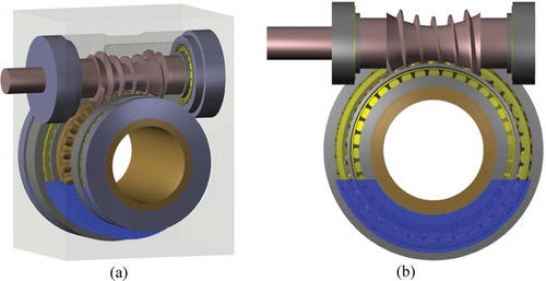
Four different MPS models for the speed reducer were created to study the flow field inside it and the lubrication performance at different rotation speeds. Key parameters are listed in Table 2 and one such model is displayed in Figure 7, which includes about 20 components. The maximum speed of our servo motor is 1440 rpm. Considering that capacity limitation of the motor, four rotation speeds, 300, 600, 900, and 1200 rpm were selected for this study. To ensure the accuracy of the simulations, the particle diameter was set to 0.7 mm, which equals one-third of the narrowest space within the casing. The initial timesteps could be calculated from Equation (9). Circumferential speeds of the worm and the worm gear shaft at the selected rotation speeds were calculated as: 0.942 m/s for worm and 0.069 m/s for worm gear shaft at 300 rpm; 1.884 m/s for worm and 0.138 m/s for worm gear shaft at 600 rpm; 2.826 m/s for worm and 0.207 m/s for worm gear shaft at 900 rpm; 3.768 m/s for worm and 0.276 m/s for worm gear shaft at 1200 rpm.

Table 2. MPS model parameters.

Model	Rotation speed of worm	Initial timestep	Particle diameter	Particle number
1	300 rpm	2 × 10^−4 s	0.7 mm	629,942
2	600 rpm	1 × 10^−4 s	0.7 mm	629,942
3	900 rpm	6.65 × 10^−5 s	0.7 mm	629,942
4	1200 rpm	5 × 10^−5 s	0.7 mm	629,942

Figure 7. MPS models of the speed reducer and the lubricant.

4. Results and discussion

4.1. Simulation results

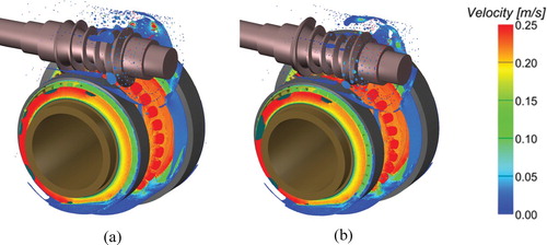
The lubrication performance is indicated by the churning loss and the oil distribution, including the velocity field and pressure distributions. Since the rotation speed of the worm gear is quite low, the velocity of the churned oil is also low. We set the highest plot scale limit as 0.25 m/s when generating the velocity field plots so that it is easy to observe and compare the results. Figure 8 shows velocity field distributions of the worm gear set with cylindrical and conical rollers under a speed of 600 rpm.

Figure 8. Velocity distributions at 600 rpm. (a) cylindrical rollers; (b) conical rollers.

As will be fully demonstrated in the next section, it was observed from experiments that a certain amount of lubricant attached to the worm thread surfaces at the speeds of 300 and 600 rpm. When increasing the speed of the worm, the lubricant was splashed onto inner walls of the casing.

In gear transmission, a large amount of heat would be generated due to the friction between the contacting tooth surfaces. In theory, the higher the velocity the lubricant is, the more heat will be carried away during the same time period, which is more beneficial for lubrication. From Figure 8 it can be seen that high velocities of the lubricant occur at the surfaces of the rollers and are evenly distributed along those surfaces. The velocity distribution on the cylindrical rollers is very close to that on the conical rollers. In other words, both the cylindrical and conical rollers can achieve ideal velocity distributions on their surfaces. In addition, the increase in the oil velocity favors the flow of oil and small substances on the tooth surfaces and can be removed easily by the oil. Figure 8 indicates that for both rollers, the maximum velocity occurs at the beginning position of the engagement, which is helpful for excluding the substances and other inclusions from the worm-gear engagement so as to attain an improved lubrication performance.

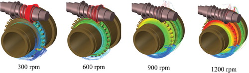
During the lubrication process, the oil pressure will be generated due to the resistance that the oil must overcome in the lubrication lines to reach the lubricated components. Such a pressure will lead to a power loss. The pressure distribution plot (Figure 9) indicates that maximum lubricant pressure occurs at the bottom of the gearbox for both types of rollers. It is thus expected that a certain amount of power loss will occur at those places, and this amount is positively related to the maximum oil pressure. It also needs to be mentioned that in a gearbox, the maximum pressure should not occur at the oil sump during operation but will appear at the tooth flanks.

Figure 9. Pressure distributions at 600 rpm. (a) cylindrical rollers; (b) conical rollers.

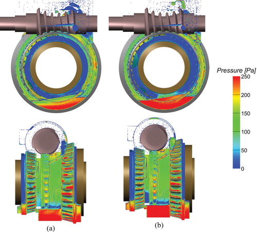
It is hard to tell from Figure 9 what type of roller yielded a higher pressure and thus led to more power loss. In order to better distinguish the pressure generated at the bottom of the casing, we partitioned the casing bottom into three subareas at the bottom of the bearing 1, the bottom of the worm wheel, and the bottom of the bearing 2, as shown in Figure 10.

Figure 10. Subareas at the bottom of the casing.

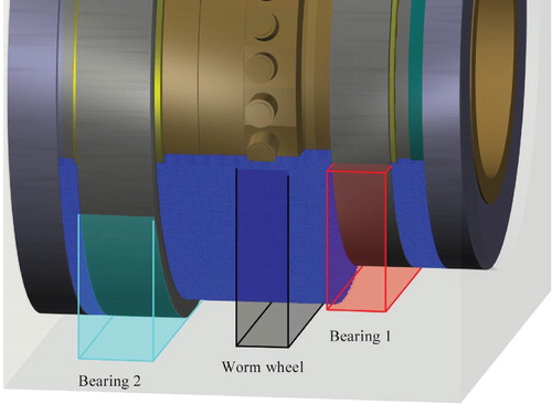
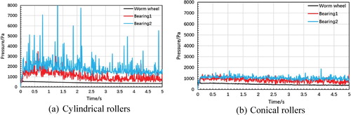
The average pressure distribution as well as pressure distributions on different sub areas are plotted in Figures 11 and 12. Figure 11 reveals the relationship between the average pressure and the rotation speed. From that figure, it can be found that for both roller types, the pressure at the bottom of the casing increased as the rotation speed climbed. Figure 12 compares the pressures at different subareas. According to that figure, the average oil pressure on the worm gear, bearing 1, and bearing 2 of the cylindrical roller speed reducer are 416.89, 1090.52, and 1895.54 Pa, respectively; while the average pressure on the same components of the conical roller speed reducer are 459.78, 851.46, and 1055.90 Pa, respectively. Thus, it can be determined that the pressures generated on the worm gears of the two types of the speed reducer are close to each other while the pressures caused on the two bearings for the worm gear with the cylindrical rollers are clearly higher than those on the bearings of the worm gear with the conical rollers. Therefore, it can be deduced that the conical roller speed reducer should have a more efficient transmission than the cylindrical roller speed reducer, which agrees well with the experimental results.

Figure 11. Distributions of pressure under different rotation speeds. (a) cylindrical rollers; (b) conical rollers.

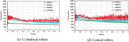
Figure 12. Pressure distributions on subareas of the casing bottom area. (a) cylindrical rollers; (b) conical rollers.

To achieve an ideal lubrication condition, every rotating part within the casing should be in direct contact with the lubricant. We obtained the lubricant distribution profiles for the speed reducer with the two types of rollers through numerical simulation, as shown in Figure 13. That figure clearly shows that for both types of rollers, there is enough lubricant oil along the engagement surfaces between the worm and the gear, and on the bearings. The worm shaft bearings were lubricated through the oil splashed by the worm gear and the splashed oil is also reflected in that figure. In order to compare the influence of the roller type on the oil distribution, therefore the lubrication condition, we selected a meshing area (Figure 14) to count the number of lubricant particles. The quantity of oil in the meshing area is a key indicator of the lubrication behavior of the worm/worm gear transmission. More lubricant in the meshing zone will facilitate the generation of oil films on tooth surfaces so as to reduce gear tooth friction and carry away more heat. Figure 15 displays the numbers of lubricant particles obtained from the two types of rollers at four rotation speeds.

Figure 13. Distributions of lubricant oil at 600 rpm (a) cylindrical rollers; (b) conical rollers.

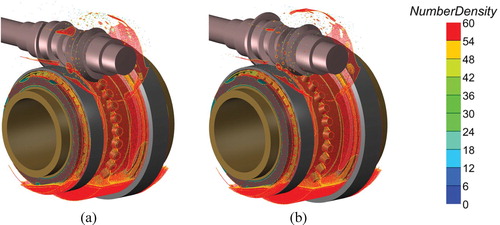
Figure 14. Selected meshing area for counting the number of lubricant particles.

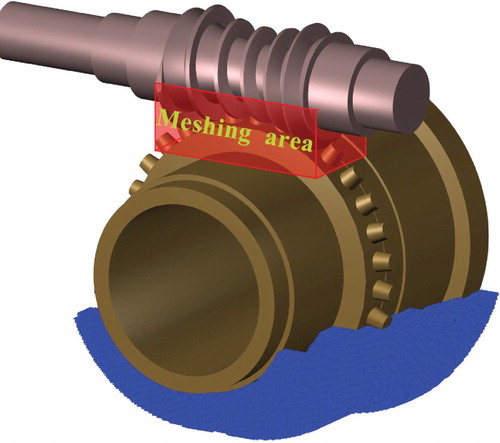
Figure 15. Numbers of lubricant particles at different rotation speeds. (a) cylindrical rollers; (b) conical rollers.

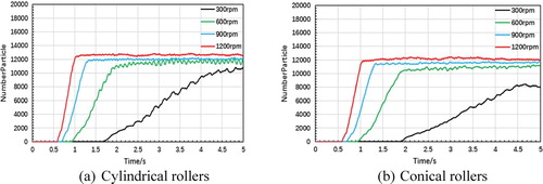
Figure 15 shows that at low speeds, the number of oil particles distributed in the meshing area of the cylindrical roller enveloping speed reducer are more than that of the conical roller enveloping speed reducer. However, when the speed reaches and exceeds 600 rpm, the numbers of lubricant particles generated from these two types of roller enveloping speed reducers are very close to each other. Theoretically, the more lubricant particles a meshing area has, the more work is needed to churn them, and the more power losses are incurred. Also, the higher the speed is, the quicker that the amount of lubricant in the meshing zone reaches equilibrium. As shown in Figure 15, the amount of lubricant in both speed reducers achieved equilibrium after 4.5 s as the rotation speed was 300 rpm; after 2 s when the speed was 600 rpm, after 1.25 s when it was 900 rpm; and after 1 s when it was 1200 rpm.

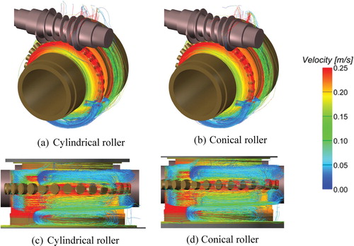
The rotation of the worm gear causes the lubricant to flow. During the churning process, the rapid and irregular motion of the lubricant at the bottom of the casing may lead to turbulence, which in turn causes the churning losses when the worm gear is immersed in the turbulent lubricant flow. Figure 16 shows trajectories of the oil during the operation of the speed reducer. From Figure 16(a,b) we can find that the turbulence formed on the worm thread surfaces is weaker than that formed on the worm gear roller surfaces. The trajectories indicate that most of the lubricant drawn by the rotating worm splashed out when it approached the top of the casing. Figure 16(c,d) display the turbulent flow generated at the bottom of the casing of the speed reducer with the cylindrical and conical rollers, respectively. From those figures it can be seen that the direction of oil flow is the same as that of rotation of the worm gear and the oil flow trajectories obtained from the speed reducers with cylindrical and conical rollers are similar to each other.

Figure 16. Distribution of trajectories of the lubricant oil. (a) cylindrical rollers; (b) conical rollers.

To closely inspect the influence of roller type and rotation speed on the variation of the trajectories of lubricant oil, we present simulation plots to show the distribution of the oil trajectories at four rotation speeds: 300, 600, 900, and 1200 rpm. From Figures 17 and 18 we can find that when the speed rose, the lubricant trajectories largely centered on the worm gear roller surfaces and relatively strong turbulences were generated. This phenomenon indicates that as the rotation speed rises, the churning losses also increases.

Figure 17. Distributions of lubricant trajectories at different speeds for the cylindrical roller reducing device.

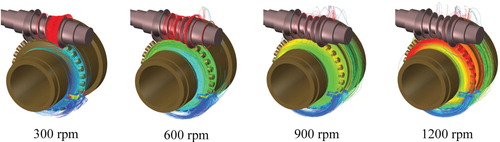
Figure 18. Distributions of lubricant trajectories at different speeds for the conical roller reducing device.

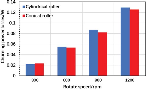
The churning power losses of the speed reducers with conical and cylindrical rollers at different rotation speeds were calculated from numerical simulations and displayed in Figure 19. From that figure it can be deduced that the churning losses increased when the rotation speed went up. At low speeds (<600 rpm), the churning losses of the two speed reducers were close to each other. As the speed exceeded 600 rpm, the churning losses of the cylindrical roller speed reducer were slightly higher than those of the conical roller speed reducer. Therefore, the conical roller speed reducer provides a better lubrication performance.

Figure 19. Churning power losses for reducers at different rotation speeds.

4.2. Experimental results and comparison

The MPS method is to solve transient incompressible flows. Different from steady-state analysis, which requests convergence to a steady-state solution of the system, the transient analysis only requests the solution at each timestep converges after iterations (80–100 iterations in our simulations). Convergence graph cannot be plotted using ParticleWorks because we could not extract residuals after certain number of iterations from postprocessing. However, we plot the relationship between the number of timesteps and the simulation time (Figure 20). From the linear relationship shown in Figure 20 it can be deduced that the simulation is conducted at the calculated initial timestep and the solution at each timestep converges. This is because if the solution for a certain timestep does not converge, the timestep will be automatically reduced and the linear relationship will not be preserved. In order to further verify the convergence and accuracy of the simulation results, as well as to validate the MPS models and CFD simulation approach, an experimental study was conducted. A speed reducer with cylinder rollers and a reducer with conical rollers were prototyped based on their design parameters following an optimal process presented by Deng et al. (2020c). A test bed was established for testing and observing the lubrication performance of these two speed reducers (Figure 21) and Figure 22 shows the speed reducer before testing. During the tests, transmission efficiencies of these two reducers were estimated using the input and output torques detected by sensors. As the CFD data suggested that the churning losses of the speed reducer with conical rollers were less than those of the one with cylindrical rollers, we would expect that the conical roller reducer has a higher transmission efficiency than the cylindrical roller reducer does.

Figure 20. Relationship between number of timestep and computing time.

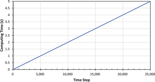
Figure 21. Speed reducer, test bed, and other facilities for the experimental study (1) motor, (2) input torque sensor, (3) speed reducer, (4) output torque sensor, and (5) loader.

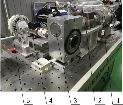
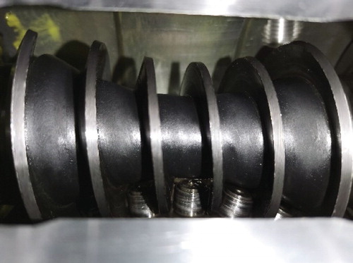
Figure 22. Roller enveloping speed reducer before testing.

The transmission efficiency was calculated as the ratio of the output power to the input power of the two speed reducers with cylindrical and conical rollers. The input/output power was calculated as the product of the torque and rotation speed at the input/output shaft (power (kW) = torque (N m) × speed (rpm)/9550). Steps of determining the transmission efficiency are: (1) set the rotation speed of the servo motor to 300 rpm; (2) confirm that the magnetic powder loader was unloaded and start the testing platform; (3) adjust the magnetic powder loader to gradually increase the applied loading from 1 to 50 N m with an increment of 1 N m and record all transmission efficiencies; (4) change the rotation speed to 600, 900, and 1200 rpm and repeat steps (2) and (3).

To capture the distribution of lubricant in the casing, we conducted following steps. (1) Cleared remnant lubricant within the speed reducers, especially if the lubricant attached to the surface of the worm; (2) added a red liquid into the lubricant oil for better visualization; (3) poured a proper amount of the mixed lubricant into the casing of the reducers so that one-third of the height of the worm gears was immersed in the lubricant, as in the simulations; (4) set the rotation speed of the servo motor to 300 rpm and started it, captured splashing of the lubricant using a high speed camera; (5) reset the rotation speed to 600 rpm and repeated step (4) to compare the splashing of the lubricant at the two rotation speeds.

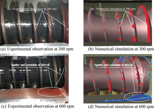
As shown in Figure 23(a), when the rotation speed was 300 rpm, a layer of lubricant was attached onto the worm tooth surface at the starting end of engagement. As the speed rose to 600 rpm, an amount of oil was observed to splash on the right side and a quantity of oil began to gather below the worm, particularly on the right side (Figure 23(c)). CFD simulations also revealed similar phenomena, as displayed in Figures 23(b,d). In other words, the CFD simulation results agreed quite well with the experimental observations. The colorful particles in Figure 23(c,d) represent particles with different velocities (please refer to Figure 8). The velocity of particles is colored in those figures to indicate the tendency for oil splashing. It’s worth mentioning that the volume of oil in Figure 23 was estimated as the number of oil particles times the volume of an individual particle, and the number of particles can be obtained from postprocessing the simulation results.

Figure 23. Lubricate distributions observed from experiments and acquired from CFD simulations. (a) Experimental observation at 300 rpm; (b) Numerical simulation at 300 rpm; (c) Experimental observation at 600 rpm; (d) Numerical simulation at 600 rpm.

Unfortunately, the churning losses calculated from the simulations cannot be directly compared to existing experimental data. The reason is that the power losses measured from experiments include tooth friction loss, seal friction loss, and bearing friction loss. Those considerable friction losses would exist even a transmission device is in an ‘empty’ load condition. In order to directly compare the simulation results with the experimental data, the aforementioned friction losses have to be excluded from the experimental power losses.

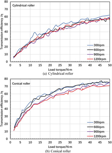
 Figure 24 compares the transmission efficiency of the two speed reducers at four different rotation speeds. It can be seen from that figure that the transmission efficiency of the speed reducer with conical rollers was greater than the reducer with cylindrical rollers.

Figure 24. Comparison of transmission efficiency of two types of speed reducer.

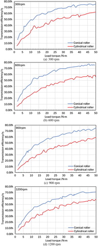
 Figure 25 illustrates the effect of the rotation speed on the transmission efficiency. From that figure it can be found that for both types of reducer, their efficiency slightly decreased as the rotation speed increased but the influence of the speed was very small. The same conclusions were also drawn from the simulation analysis.

Figure 25. Effect of rotation speed on transmission efficiency.

5. Conclusion

This paper presents a combined theoretical-experimental-computational (using ParticleWorks) study to investigate the impacts of the roller shape and other factors such as rotation speed on the lubrication behavior of precision roller enveloping speed reducers. The conclusions drawn from this study are:

1. The shape of the roller has a considerable influence on the lubrication performance through affecting the lubricating film formation between mating surfaces and the oil churning.

2. The CFD simulation has proven that the conical roller reducer has slightly lower churning losses, whereas the equation for lubrication angle derived by Deng has proven its potential for a better lubrication performance.

3. The transmission efficiency of the speed reducer with conical rollers is higher than that of the reducer with the cylindrical rollers, as confirmed by both numerical and experimental analysis.

4. Both the cylindrical and conical rollers can lead to ideal velocity distribution on their surfaces, and the maximum velocity occurs at the beginning position of the engagement, which is helpful for removing substances and other inclusions from the worm-gear engagement.

5. The pressures generated on the worm gears with the two types of the rollers are close to each other while the pressures on the two bearings of the worm gear with the cylindrical rollers are evidently higher than those on the bearings of the worm gear with the conical rollers.

6. For speed reducers with both types of rollers, the churning losses increase as the rotation speed increases. At low speeds (<600 rpm), the churning losses of the two speed reducers are close to each other and at high speeds (>600 rpm), the churning losses of the speed reducer with the conical rollers are slightly lower than those of the reducer with the cylindrical rollers.

7. The MPS method can effectively eliminate the error caused by tangled meshes and remeshing when the material being simulated moves around and is an effective tool for simulation of lubrication of complicated worm and worm gear surfaces.

8. In the assessment of lubrication behavior of the speed reducer, the lubrication conditions of bearings and other components need to be considered in addition to the lubrication of transmission parts such as worms and gears. In traditional spur gear reduction units, the churning losses of the reducer are mainly caused by the churning losses of the gears, while the losses of due to the bearings can be ignored. However, in the present roller enveloping speed reducer that uses a worm gear transmission, the worm gear rotates very slow due to its high transmission ratio (30:1), the churning losses due to the rotation of the worm gear are limited. Meanwhile, the bearings for the worm gear are immersed in the lubricant, so their churning losses must be considered when calculating the total churning losses of the device.

In the future, a novel experimental approach needs to be designed to directly measure the churning power losses (exclusive of the friction losses) so that a quantitive analysis can be performed to directly compare the churning losses obtained from simulations to those from experiments. A tripod will be equipped to improve the camera system so that the oil distribution can be observed from the exact same position as in the simulations (Figure 23). The present study only compares the lubrication behavior of the high precision enveloping speed reducers with cylindrical and conical rollers. Based on the outcomes of this study, the design of roller enveloping speed reducers will be further improved to achieve optimal lubrication performance.

Disclosure statement

No potential conflict of interest was reported by the author(s).

Additional information

Funding

This work was supported by Sichuan Distinguished Youth Fund: [grant number 19JCQN]; National Natural Science Foundation of China: [grant number 51875479].

References

- Akbarian, E., Najafi, B., Jafari, M., Ardabili, S. F., Shamshirband, S., & Chau, K.-W. (2018). Experimental and computational fluid dynamics-based numerical simulation of using natural gas in a dual-fueled diesel engine. Engineering Applications of Computational Fluid Mechanics, 12(1), 517–534. https://doi.org/10.1080/19942060.2018.1472670
- Chen, S.-W., & Matsumoto, S. (2016). Influence of relative position of gears and casing wall shape of gear box on churning loss under splash lubrication condition – some new ideas. Tribology Transactions, 59(6), 993–1004. https://doi.org/10.1080/10402004.2015.1129568
- Concli, F., & Gorla, C. (2017). Numerical modeling of the churning power losses in planetary gearboxes: An innovative partitioning-based meshing methodology for the application of a computational effort reduction strategy to complex gearbox configurations. Lubrication Science, 29(7), 455–474. https://doi.org/10.1002/ls.1380
- de Moura, C. A., & Kubrusly, C. S. (2013). The courant-friedrichs-lewy (CFL) condition: 80 years after its discovery. Birkhauser.
- Deng, X.-Q., Liu, Y.-C., & He, G. (2019b, April). Design and assessment of an antibacklash single roller enveloping hourglass worm gear (SAE Technical Paper 2019-01-1071). Proceedings of SAE 2019 World Congress Experience, Detroit, MI: Society of Automotive Engineers.
- Deng, X.-Q., Wang, S.-S., Hammi, Y., Qian, L.-M., & Liu, Y.-C. (2020b). A combined experimental and computational study of lubrication mechanism of high precision reducer adopting a worm gear drive with complicated space surface contact. Tribology International, 146, 106261. https://doi.org/10.1016/j.triboint.2020.106261
- Deng, X.-Q., Wang, J.-G., & Horstemeyer, M. F. (2012). Parametric study of meshing characteristics with respect to different meshing rollers of the anti-backlash double-roller enveloping worm gear. Journal of Mechanical Design, 134(8), 081004 (1–12). https://doi.org/10.1115/1.4006829.
- Deng, X.-Q., Wang, S.-S., Wang, S.-K., Wang, J., Liu, Y.-C., Dou, Y.-Q., & He, G. (2020a). Lubrication mechanism in gearbox of high-speed railway trains. Journal of Advanced Mechanical Design, Systems, and Manufacturing (Machine Design & Tribology), 14(4). https://doi.org/10.1299/jamdsm.2020jamdsm0054.
- Deng, X.-Q., Wang, J., Wang, S.-K., Wang, S.-S., Liu, Y.-C., & He, G. (2019c). A comparison study of anti-backlash single- and double-roller enveloping hourglass worm gear. Chinese Journal of Mechanical Engineering, 56(3), 88–95. https://doi.org/10.3901/JME.2020.03.088.
- Deng, X.-Q., Wang, J., Wang, S.-K., Wang, S.-S., Liu, Y.-C., & He, G. (2019d, November). Meshing characteristics and engagement of anti-backlash single- and double-roller enveloping hourglass worm gear (IMECE2019-11332). Proceedings of the ASME 2019 International Mechanical Engineering Congress and Exposition, Salt Lake City, UT: American Society of Mechanical Engineers.
- Deng, X.-Q., Wang, J., Wang, S.-K., Wang, S.-S., Liu, Y.-C., & He, G. (2020c). An optimal process of machining complex surfaces of anti-backlash roller enveloping hourglass worms. Journal of Manufacturing Processes, 49, 472–480. https://doi.org/10.1016/j.jmapro.2019.12.016
- Deng, X.-Q., Wang, J., Wang, S.-K., Wang, S.-S., Wang, J.-G., Li, S.-C., Liu, Y.-C., & He, G. (2019a). Investigation on the backlash of roller enveloping hourglass worm gear: Theoretical analysis and experiment. Journal of Mechanical Design, 141(5), 053302 (1–11). https://doi.org/10.1115/1.4042155.
- Duan, G.-T., Chen, B., Koshizuka, S., & Xiang, H. (2017). Stable multiphase moving particle semi-implicit method for incompressible interfacial flow. Computer Methods in Applied Mechanics and Engineering. https://doi.org/10.1016/j.cma.2017.01.002.
- Duan, G.-T., Yamaji, A., & Koshizuka, S. (2019). A novel multiphase MPS algorithm for modeling crust formation by highly viscous fluid for simulating corium spreading. Nuclear Engineering and Design, 343, 218–231. https://doi.org/10.1016/j.nucengdes.2019.01.005
- Ghalandari, M., Bornassi, S., Shamshirband, S., Mosavi, A., & Chau, K.-W. (2019). Investigation of submerged structures’ flexibility on sloshing frequency using a boundary element method and finite element analysis. Engineering Applications of Computational Fluid Mechanics, 13(1), 519–528. https://doi.org/10.1080/19942060.2019.1619197
- Hu, X., Jiang, Y., Luo, C., Feng, L., & Dai, Y. (2019). Churning power losses of a gearbox with spiral bevel geared transmission. Tribology International, 129, 398–406. https://doi.org/10.1016/j.triboint.2018.08.041
- Ji, Z., Stanic, M., Hartono, E. A., & Chernoray, V. (2018). Numerical simulations of oil flow inside a gearbox by smoothed particle hydrodynamics (SPH) method. Tribology International, 127, 47–58. https://doi.org/10.1016/j.triboint.2018.05.034
- Jiang, Y., Hu, X., Hong, S., Li, P., & Wu, M. (2019). Influences of an oil guide device on splash lubrication performance in a spiral bevel gearbox. Tribology International, 136, 155–164. https://doi.org/10.1016/j.triboint.2019.03.048
- Khayyer, A., & Gotoh, H. (2009). Modified moving particle semi-implicit methods for the prediction of 2D wave impact pressure. Coastal Engineering, 56(4), 419–440. https://doi.org/10.1016/j.coastaleng.2008.10.004
- Koshizuka, S., & Oka, Y. (1996). Moving-particle semi-implicit method for fragmentation of incompressible fluid. Nuclear Science and Engineering, 123(3), 421–434. https://doi.org/10.13182/NSE96-A24205
- Koshizuka, S., Tamako, H., & Oka, Y. (1995). A particle method for incompressible viscous flow with fluid fragmentation. Computational Fluid Dynamics Journal, 4, 29–46.
- Laruelle, S., Fossier, C., Changenet, C., Ville, F., & Koechlin, S. (2017). Experimental investigations and analysis on churning losses of splash lubricated spiral bevel gears. Mechanics & Industry, 18(4). https://doi.org/10.1051/meca/2017007
- Leprince, G., Changenet, C., Ville, F., & Velex, P. (2012). Investigations on oil flow rates projected on the casing walls by splashed lubricated gears. Advances in Tribology, 365313, 1–7. https://doi.org/10.1155/2012/365414
- Li, Y., Pi, B., Wang, Y., Liu, L., & Chen, X. (2018). Analysis and validation of churning loss of helical gear based on moving particle semi-implicit method. Journal of Tongji University (Natural Science), 46(3), 368–372. https://doi.org/10.11908/j.issn.0253-374x.2018.03.013.
- Litvin, F. L., & Fuentes, A. (2004). Gear geometry and applied theory. Cambridge University Press.
- Liu, H., Standl, P., Sedlmair, M., Lohner, T., & Stahl, K. (2018). Efficient CFD simulation model for a planetary gearbox. Forschung im Ingenieurwesen, 82(4), 319–330. https://doi.org/10.1007/s10010-018-0280-2
- Motohashi, H., Emura, T., & Sakai, T. (1986). A study on zero-backlash reduction mechanism. Bulletin of JSME, 29(255), 3189–3194. https://doi.org/10.1299/jsme1958.29.3189
- Prometech Software. (2016). ParticleWorks theory manual.
- Renjith, S., Srinivasa, V. K., & Shome, B. (2015). CFD based prediction of spin power loss of automotive differential system. SAE International Journal of Commercial Vehicles, 8(2), 460–466. https://doi.org/10.4271/2015-01-2783
- Sakai, M., Shigeto, Y., Sun, X.-S., Aoki, T., Saito, T., Xiong, J.-B., & Koshizuka, S. (2012). Lagrangian-Lagrangian modeling for a solid-liquid flow in a cylindrical tank. Chemical Engineering Journal, 200–202, 663–672. https://doi.org/10.1016/j.cej.2012.06.080
- Salih, S. Q., Aldlemy, M. S., Rasani, M. R., Ariffin, A. K., Yusoff, T. M., Al-Ansari, N., Yaseen, Z. M., & Chau, K.-W. (2019). Thin and sharp edges bodies-fluid interaction simulation using cut-cell immersed boundary method. Engineering Applications of Computational Fluid Mechanics, 13(1), 860–877. https://doi.org/10.1080/19942060.2019.1652209
- Simon, V. (2008). Influence of tooth errors and misalignments on tooth contact in spiral bevel gears. Mechanism and Machine Theory, 43(10), 1253–1267. https://doi.org/10.1016/j.mechmachtheory.2007.10.012
- Zhong, C.-H., & Yang, X.-J. (2015). Driving torque reduction in linkage mechanisms using joint compliance for robot head. Chinese Journal of Mechanical Engineering, 28(5), 888–895. https://doi.org/10.3901/CJME.2015.0520.073