Research on aerodynamic optimization of high-speed train’s slipstream

Abstract

Slipstream severely affects the safety of trackside workers and equipment. With use of profile superimposition method and vehicle modeling method, parametrization of the whole train is carried out. Then, a slipstream optimization study has been performed, taking components of slipstream in different directions at the standard heights, the drag coefficient of the whole train and the volume of the driving cab as the design objectives. For each design objective, one unique ϵ-TSVR surrogate model has been constructed. Six final Pareto sets have been obtained on the base of six groups of different fitness functions by using multi-objective particle swarm method. Results reveal that the volume of the driving cab keeps almost the same, compared to the original shape. The velocity components of train-induced wind at the positions 0.2  and 1.4 m above the top of the rail, and the drag coefficient of the train are reduced by 11.6%, 33.9%, 24.7%, 25.9% and 13.0% respectively. Sensitivity analysis reveals that the length of the streamline, the height of the train and the width of the train influence significantly on the aerodynamic performance, and the train with a tall and thin streamline will benefit in reducing the slipstream and aerodynamic drag.

KEYWORDS:

• Slipstream
• ϵ-TSVR
• shape optimization
• high-speed train
• DDES

1. Introduction

The flow around high-speed trains is a kind of complicated three-dimensional, unsteady and highly turbulent flow. The vortex structures in the wake of the train could not only affect the aerodynamic performance of the trailing car, but also induce strong slipstream, causing safety problems for trackside workers and constructions. Different regulations have been made on the limitation of extreme values of slipstream in different countries. In Japan, the extreme value of the slipstream is 9 m/s. In United Kingdom, it is set to be 11.1 m/s. In Germany and France, the maximum aerodynamic load of the slipstream on the passengers is set to be 100N (Lee, 1999; Liao et al., 1999). Meanwhile, obvious requirement on the extreme value of the slipstream has also been made in TSI. As a result, sufficient consideration should be taken on the slipstream when designing new high-speed trains.

Numerical approach is a fundamental way to study fluid mechanisms. With use of steady Reynolds-Averaged method, Mou et al. (2017) studied the influence of environmental wind on the wind pressure on high building in the atmospheric boundary layer conditions. Ghalandari et al. (2019) performed a study on the wing’s flatter characteristics by the DQM method. Farzaneh-Gord et al. (2019) carried out a research on the flow characteristics inside the natural gas pipeline by use of an unsteady method. The maximum value of the slipstream usually locates in the wake region of the train, where two strong counter rotating vortices exist (Baker, 2010). These two strong vortices provide the major energy into the wake flow field. They originate from the flow separation on the trailing streamlined shape and interact severely with the ground, which proposes a high accuracy demand in corresponding numerical simulation. Due to its transient characteristics, it is crucial to adopt algorithms with high accuracy to precisely capture the correct flow details. A comparative study on wake characteristics between DES and URANS was performed by Yao et al. (2013). With use of DES and POD methods, Muld et al. (2012) successfully performed a thorough study on the vortex structures in the wake zone. Similarly, Osth et al. (2015) used LES and ROM methods to study the characteristics of vortex structures in the wake zone. In the meantime, Bell et al. (2014) also studied the vortex structures by wind tunnel experiments and demonstrated the distribution characteristics of these vortices. With use of unsteady numerical method and genetic algorithm, Muñoz-Paniagua and Garcia (2019) studied the influence of streamlined head on the side force of the trains when two trains pass by each other in crosswind conditions.

Flow separation on the trailing streamlined shape could determine the intensity of the trailing vortices. Consequently, the intensity of the slipstream in the wake region could also be affected. By optimizing the streamlined shape, the flow separation status could be improved obviously, so as to weaken the slipstream in the wake region (Bell et al., 2017). Strong transient characteristics of the wake flow could lead to severe variation of the slipstream with time. Although the time-averaged value could be used to reflect the feature of slipstream, it is unreliable to obtained the time-averaged value through a steady numerical approach. As a result, an unsteady numerical method is adopted to perform the aerodynamic optimization with the slipstream as its objective in the present study. Currently, except for the optimization on micro pressure waves (Ku et al., 2010; Ku et al., 2010), most aerodynamic optimization studies are based on steady numerical simulations (Vytla et al., 2010; Yao et al., 2014; Yao et al., 2015). Optimization based on an unsteady approach is rather rare [8]. The influence of the nose’s length on the wake flow was investigated by Bell etc. (2017) by wind tunnel experiments. Hemida and Krajnovic (2010) used the LES method to study the effect of head length and side angle on the flow field around the train under cross wind conditions. Yao et al. (2013) analyzed the impact of URANS and DES (Spalart, 2009) models on the simulation accuracy of the wake field. Wang et al. (2017) carried out a research on simulation accuracy of URANS, SAS and DES models on the train wind. Results all reveal that the DES model can simulate the flow structures in the wake field more accurately. Therefore, this paper uses DES for numerical simulation. Compared with RANS models, the computational cost of DES has increased significantly, and it is difficult to directly use optimization algorithms to carry out aerodynamic optimization to reduce the train wind. To solve this problem, this paper introduces the support vector machine regression model (Peng, 2010), and uses particle swarm optimization (Kennedy & Eberhart, 1995) and cross-validation algorithm to train the support vector machine model. In order to obtain the optimal solution set more quickly, the multi-objective particle swarm optimization algorithm is introduced, and multi-objective optimization design has been carried out with the optimization goal of reducing the train wind amplitude. Meanwhile, the relationship between the design variables and the train wind has been obtained.

Parametric design is a major difficulty for aerodynamic optimization design of high-speed trains. Current studies usually focus on some limited parameters of the streamlined shape and their relationship with the flow field around the train (Vytla et al., 2010; Yao et al., 2014, 2015, 2016). Yao et al. (2016) developed several three-dimensional parametric methods to perform the aerodynamic optimization study of high-speed trains, in which the cross section of the train is always kept constant, so that the influence of the geometry of the train body on aerodynamic performance of the train couldn’t be analyzed. It is obvious that cross section of the train gets a severe influence on the flow field around train. Taking the reduction of the train wind as the optimization objectives, more and more elaborate aspects should be considered, including the cross section of the train, the length of the streamlined shape, and the local design of the streamlined shape, so as to gain insight on the engineering design of train-wind beneficial streamlined head. As a result, in the present paper, a new parametric method has been proposed which takes the cross-section of the train into consideration on the base of the previous study (Yao et al., 2016). This new parametric study could guarantee the parametrization of a whole train.

2. Parametrization methods

2.1. Parametrization on the cross-section of the train body

Cross-section of the train body is a key factor to the geometric shape of a train, and could directly affect the aerodynamic performance of the train. Usually, the cross-section could be seen as a combination of several lines and arcs with different diameters. The key variables to control the cross-section are the height and width of the train. The profile superposition method is adopted for parametrization here, as shown in Figure 1. Since the train is design symmetrically, only half of the profile needs to be parametrized.

Figure 1. Profile superposition method of the cross-section.

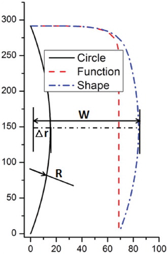
The NURBS method is a commonly used parametrization method. The profile is determined by the coordinates and weights of several control points. The more the control points, the more flexible the profile is. However, as the increase of the number of design points, parametrization becomes more and more complicated. The profile superposition method is a new parametrization method proposed in the present paper. Two profiles are provided, namely the baseline profile and the auxiliary profile. The former could be governed by the Equation (1) (Yao et al., 2016), in which, the parameter n determines the angle of chamfer between the upper and lateral profiles and c determines the width of the train. (1) $y^n+z^n=c^n;$(1)

The auxiliary profile is designed to modify the straight line in the cross-section, and could be governed by polynomial equations, circle equations, trigonometric functions or the combination of the former three kinds. Circle equation is adopted in the present paper, which is designed as (2) (2) $y^2+z^2=r^2;$(2)

The bigger the radius r is, the smaller the curvature of the arc becomes, consequently, the smaller the curvature of the cross-section after superposition is. The final width of the train, w, is controlled by c and r.

2.2. Parametrization on the streamlined shape

The streamlined shape of high-speed trains is consisted of complicated three-dimensional free surfaces. When performing parametrization of the streamlined shape, a large number of design variables are required (Yao et al., 2016). In the present paper, the vehicle modeling function (VMF) method is adopted to parametrize the streamlined shape, the details of which could be referred to in literature (Yao et al., 2014, 2015), and will not be mentioned in detail here.

Some key variables that control the deformation of the streamlined shape include the length of the streamline, the cross-section profile, the longitudinal profile, the horizontal profile, and the drainage. The governing equation of the profiles of longitudinal section and horizontal section (Yao et al., 2016) could be expressed as below: (3) $\begin{array}{rl}z(x)& ={\left(\frac{x-x_1}{x_2-x_1}\right)}^{A_1}{\left(1-\frac{x-x_1}{x_2-x_1}\right)}^{A_2}{a}_k\\ & \times {\left(1-\frac{x-x_1}{x_2-x_1}\right)}^{a_b}+g(x);\end{array}$(3) In which, $g(x)=2(z_2-z_1)(x-x_1/x_2-x_1)-(z_2-z_1)(x-x_1/x_2-x_1{)}^2$, controls the curvature and height at the ends of the curves. $x_1$and $x_2$ are the x coordinates of the starting point and ending point respectively, while $z_1$and $z_2$ are the z coordinates of starting point and ending point.

For different streamlined shapes, the curvature at the connection part between the streamline and the train body usually should be consistent. As a result, the variable which controls the deformation of the trailing part of the profile, $A_2$, is set to be constant, while the other three variables, $A_1$, $a_k$ and $a_b$ are chosen to be the design variables that control the deformation of the profile.

The parametrization of the drainage and the window on the driving cab could be referred to in literature (Yao et al., 2016). The key design variables are $D_h$ which controls the depth of the drainage and $W_h$ that controls the height of the window. Consequently, these two variables are also chosen to be design variables. In total, 12 design variables are under consideration in the present study, as shown in Table 1.

Table 1. Design variables.

Design variables	Controlling area	Design variables	Controlling area
L	Streamline length	$A_{11}$, $a_{k1}$, $a_{b1}$	Longitudinal profile of the streamline
H	Height of the cross-section	$A_{21}$, $a_{k2}$, $a_{b2}$	Horizontal profile of the streamline
c	Baseline width of the cross-section	$D_h$	Depth of the drainage
r	Superimposition width of the cross-section	$W_h$	Height of the cab window

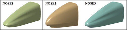
Based on the above parametrization methods, Figure 2 shows three different kinds of streamlined shapes. It could be observed that the three streamlined shapes are obviously distinct from each other. NOSE1 is broad and flat, NOSE2 is tall and thin, while NOSE3 is fusiform. All the streamlined shapes are smooth and no bumps could be found, indicating that the parametrization methods designed in the present paper could be used to generate reasonable geometric shapes with different topologies and meet the optimization requirement.

Figure 2. Different kinds of streamlined shapes.

3. Numerical methodologies

3.1. Computational algorithms, conditions and domain

As a kind of RANS/LES hybrid method, DES (Spalart, 2009) benefits in solving flow with high Reynolds number and large separations. In numerical simulations of flow around ground vehicles where large flow separation exists, DES owns higher accuracy in prediction of aerodynamic drag and flow separations. Since prominent transient characteristics exist in flow around high-speed trains, it is more reasonable to use DES to obtain more accurate flow structures as long as the computational cost is affordable (Yao et al., 2013). According to the use of different turbulence models, two different DES methods could be divided, which are the DES method based on SA turbulence model, and the DES method based on k-w or SST k-w turbulence model. However, these two kinds of DES methods both face the MSD problem and grid-induced separation problem. Consequently, Menter revised the dissipation rate $\omega$ in SST k-w model into: (4) $\begin{array}{rl}\tilde{\omega }& =\omega \varphi \end{array}$(4) (5) $\begin{array}{rl}\varphi & =max\left(\frac{l_t}{C_{\text{DES}}\mathrm{\Delta }}F,1\right)\end{array}$(5) where, $l_t=(\sqrt{k}/{\beta }^{\ast }\omega )$, $\mathrm{\Delta }$ is the maximal value between the centers of computational cell and adjacent cells. $F=1-F_2$, where $F_2$ takes the form as: (6) $F_2=\tanh \left({\left(max\left(\frac{2\sqrt{k}}{{\beta }^{\ast }\omega d},\frac{500v}{d^2\omega }\right)\right)}^2\right)$(6)

When $\varphi =1$, the RANS model is selected while LES model is chosen when $\varphi >1$. (7) $C_{\text{DES}}=C_{\text{DES,}k\text{ - }\omega }{F}_1+C_{\text{DES,}k\text{ - }\epsilon }(1-F_1)$(7)

In which, $C_{\text{DES,}k\text{ - }\omega }$ and $C_{\text{DES,}k\text{ - }\epsilon }$ are set to be 0.78 and 0.61 respectively. (8) $\begin{array}{rl}{F}_1& =\tanh \\ & \times \left({\left[min\left(max\left(\frac{\sqrt{k}}{0.09\omega d},\frac{500v}{d^2\omega }\right),\frac{2k}{d^2\text{C}{\text{D}}_{k\omega }}\right)\right]}^4\right)\end{array}$(8)

In which, $d$ is the distance between the first cell and the wall, while $v$ is the kinetic viscosity coefficient. (9) $\text{C}{\text{D}}_{k\omega }=max\left(\frac{1}{\omega }\mathrm{\nabla }k\cdot \mathrm{\nabla }\omega ,{10}^{-20}\right)$(9)

There is a relative movement between the train and ground. When performing the numerical simulations, the train is usually kept stationary, while the incoming air is flowing with a speed same to the running speed of the train but with opposite direction. The ground is set as the moving wall, with the same speed of the incoming flow (Guo et al., 2016). In the present paper, the same methodology is adopted for the simulation of flow field around the train.

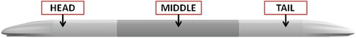
The computational model is a 1:1 scaled simplified model with three carriages. The geometry of the leading and trailing car is the same, while the inter-connection parts between the carriages, the bogies, and the pantographs are all neglected, as shown in Figure 3.

Figure 3. Computational model.

The turbulence model used with DDES is the SST k-w two-equation model. The temporal terms for all of the DDES simulations are discretized by using a second-order implicit scheme. The diffusive and sub-grid fluxes are discretized with a second-order central difference scheme. The convective term was discretized using a second-order upwind scheme.

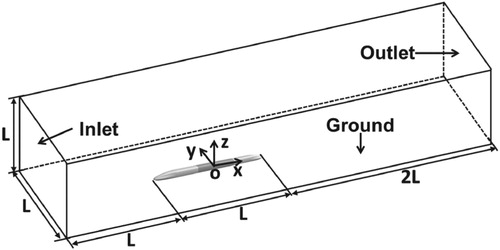
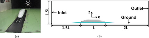
Figure 4 shows the computational domain, where the x axis is the running direction of the flow, z axis is the height direction of the train, and y axis could be determined by the right-hand rule. Taking the length of the whole train L as the characteristic length, the distance between the inlet boundary and the leading nose is L, and that between the trailing nose and the outlet boundary is 2L. The width and height of the domain are both L. The velocity inlet and pressure outlet boundaries are utilized for the inlet and outlet boundaries respectively. The incoming velocity is set to be 350 km/h. For the ground, due to its relative movement with the train, a moving wall condition with the speed of the incoming flow is prescribed. The rest far field boundaries are all set to be slip wall.

Figure 4. Computational domain.

3.2. Numerical validation

To validate the prediction accuracy of the numerical algorithms, a wind tunnel experiment has been carried out on a simplified train model. The wind tunnel is a low speed open wind tunnel with a 8 m × 6 m cross section in Mianyang, Sichuan Province. The turbulence intensity of the incoming flow is 0.2%. The installation of the train model and the test section of the wind tunnel are shown in Figure 5. The train model is fixed with the subgrade by the force-measuring balances, which are mounted on the geometry center of each carriage. They are place on a turntable, which could be used to adjust the angle of the train model and the incoming flow.

Figure 5. The train model and the side view of the wind tunnel: (a) Train model; (b) Side view of the wind tunnel.

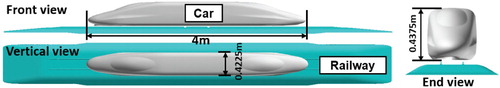
As Figure 6 shows, the train model is a quite simplified model. It only consists of a leading streamline, a trailing streamlined and a small part of train body. The inter-connection part, bogies and pantographs are not included in this model. The scaled ratio of this train model is 1:8. The total length of this model is 4 m, and its height and width are 0.4375 and 0.4225 m respectively. To validate the prediction accuracy of DDES model in large flow separation conditions, the yaw angle of the model is set to be 30°. In the wind tunnel test, aerodynamic loads are measured by force-measuring balances mounted on the geometry center of each carriage, while surface pressure is tested by the pressure probes on the train surface. The velocity of the incoming flow is 45 m/s. Taking the height of the model as the reference length, the Reynolds number is 1.28 × 10⁶.

Figure 6. Baseline train model for wind tunnel test.

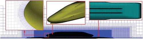
The commercial CFD software STAR-CCM+ is utilized for mesh generation and numerical simulation. The hybrid Cartesian/prism grids are adopted and 18 layers of prism grids are generated with an increasing ratio of 1.1 and a total length of 30 mm, which keeps the value of y+ of the first layer near the train surface around 30∼50. The mesh is locally densified to capture the flow details around the train. The minimum size of cells in the densified zone is 10 mm. The total amount of grids is 31.84 million. The spatial and surface distributions of mesh in different regions are shown in Figure 7.

Figure 7. Spatial and surface distributions of mesh in different regions.

To facilitate the following analysis, if no further explanation is given, the dimensionless form will be used for the aerodynamic loads of the train, which are listed as follows:

pressure coefficient, (10) $C_p=P/0.5\rho V^2$(10) drag coefficient, (11) $C_d=F_d/0.5\rho V^{2}S$(11) lateral force coefficient, (12) $C_s=F_s/0.5\rho V^{2}S$(12) lift coefficient, (13) $C_l=F_l/0.5\rho V^{2}S$(13)

In which, P is the relative pressure, ρ is the density of the incoming flow, which takes the value of 1.225 kg/m³, V is the velocity of incoming flow and S is the maximum area of the cross section of the train model.

In wind tunnel test, the surface pressure and aerodynamic loads of the train model are obtained through steady measurement. As a result, the time-averaged value is considered when performing numerical simulations. Figure 8 shows the comparison of pressure coefficients in the longitudinal and cross-sectional profiles between experimental and numerical results. It could be seen that numerical results agree well with the experimental results, indicating that the numerical algorithms used in the present paper could precisely predict the flow information on the surface of the train.

Figure 8. Comparison of pressure coefficients between experimental and numerical results: (a) Longitudinal profile; (b) Cross-sectional profile.

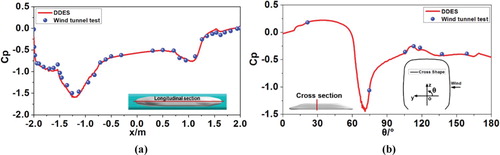
Table 2 shows the comparison of time-averaged aerodynamic loads in wind tunnel test and DDES simulations. It could be seen that the errors of C_d and C_s are 1.57% and 1.8%, respectively. The error of C_l is a little larger, which is 3.99%. Results reveal that the numerical algorithms and mesh configuration in the present study could obtain the turbulent structures in large flow separation conditions and could be used for simulation of flow field around high-speed trains.

Table 2. Comparison of aerodynamic loads between experimental and numerical simulations.

	Cd	Cs	Cl
Wind Tunnel	−0.250	3.277	3.895
DDES	−0.254	3.219	4.057
Error	1.57%	1.80%	3.99%

4. Influence of the shape simplification on slipstream

4.1. Simplification of the train model

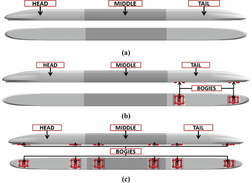
It is commonly found in reality that high-speed trains operate with 8 or 16 carriages. The key components that affect the flow around the trains include the geometric shape of the train, the bogies, the inter-connection parts and pantographs. Guo et al. (2016) performed a thorough study on the slipstream of high-speed trains with different carriages, and found that the number of carriages, the structures underneath the train and the inter-connection parts played an important role on the slipstream. It would be a more reasonable way to take the train model with all the carriages into consideration to study the slipstream. However, due to the complexity of the geometric shape of trains, the computational cost would be unaffordable when using DDES to study the slipstream problem. In the present paper, the train model with three carriages will be considered, to greatly reduce the computational cost. Compared to other components, the bogies own more complicated shape and affect greatly on the flow around the train, especially the flow underneath the train body (Gao et al., 2019; Wang et al., 2018a, 2018b). As a result, the influence of bogies on the slipstream is mainly discussed in this section, to determine a better way for the simplification of bogies.

Figure 9 shows the three ways to simplify the train model, which are the completely simplification model, the model considering the bogies on the trailing car only, and the model taking all the bogies into consideration. To facilitate the following discussion, these three models are named SP1, SP2 and SP3 respectively.

Figure 9. Three ways to simplify the train model: (a) SP1; (b) SP2; (c) SP3.

4.2. Characteristics of the slipstream

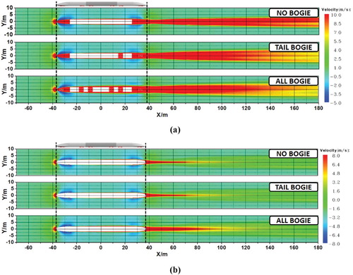
Figure 10 shows contour of x component of velocity, V_x, at different heights for the three simplification models. It could be seen that V_x distributes symmetrically at the lateral sides of the train. Negative velocity exists around the leading and trailing nose, indicating that the induced wind flows oppositely with the running train. The peak value of the slipstream at the leading nose is slightly higher, while the induced wind around the trailing nose joins the wake flow along the horizonal profile of the train surface. At the same x coordinate, V_x with the height of 0.2 m (V_x-0.2) is obviously larger than that with the height of 1.4 m (V_x-1.4). Focusing on the slipstream at the same height, maximum slipstream occurs at the height of 0.2 m. As the flow goes away from the trailing nose, the slipstream tends to propagate much wider (in y direction). However, at the height of 1.4 m, just as Figure 12(b) shows, the slipstream tends to be weaker and weaker in the wake region. The slipstream tends to be much narrower when going away from the trailing nose, indicating that trigonal distribution of V_x exists at the cross-section in the wake region. This type of distribution could also be seen as a proof to the rationality of the requirement of slipstream in TSI 1302–2014 (TSI, 1302, 2014), which is, the limitation value of V_x at the height of 0.2 m is higher than that at the height of 1.4 m.

Figure 10. Contour of V_x at different heights: (a) H=0.2 m; (b)H=1.4 m.

The bogies underneath the leading car could affect the flow around the train directly. Influence of the bogies underneath the middle car could be found at the height of 0.2 m, while could be neglected at the height of 1.4 m. By contrast, the influence of the bogies under the trailing car should must be paid enough attention to for both heights. By taking a closer look, it could be found that the wake region is greatly disturbed by the bogies under the trailing car while their influence on the leading and middle car is relatively smaller.

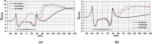
Figure 11 shows the distribution of V_x at different heights for the three simplification models. Similar distribution could be observed at different heights. Peak V_x occurs at the leading and trailing nose, while the slipstream near the middle carriage is relatively smaller. However, for the distribution in the wake region, remarkable difference could be found at different heights. V_x-0.2 is obviously larger than V_x-1.4 in the wake region. V_x-1.4 is closely related to the simplification way. For SP1 V_x-1.4 in the wake region is smaller than that around the leading and trailing nose. While for SP2 and SP3, the maximum value of V_x-1.4 in the wake region is very close to that around the leading and trailing nose. For the slipstream around the middle car at the height of 0.2 m, V_x-0.2 increases gradually for SP3 while it keeps almost constant for SP1 and SP2. Considering the distribution of slipstream in the wake region at different heights, SP2 and SP3 are very close to each other. When performing shape optimization in the present paper, the influence on the maximum value of the slipstream should be mainly considered. As a result, if taking V_x as the optimization objective, SP2 will be the best simplification model.

Figure 11. Distribution of V_x at different heights: (a) H=0.2 m; (b)H=1.4 m.

Similarly, the influence of the three models on V_y at different heights is also under investigation, as shown in Figure 12. Due to the symmetry design of high-speed trains, V_y distributes anti- symmetrically on the lateral sides. Meanwhile, V_y at the leading and trailing nose is also anti-asymmetrically distributed at the same side. Compared to the wake region, V_y around the leading and trailing nose is obviously larger. Furthermore, the area influenced by V_y at the height of 0.2 m is larger than that at the height of 1.4 m. It can be seen that the bogies have weak influence on the distribution of V_y, but only affect the adjacent zone.

Figure 12. Contour of V_y at different heights: (a) H=0.2 m; (b)H=1.4 m.

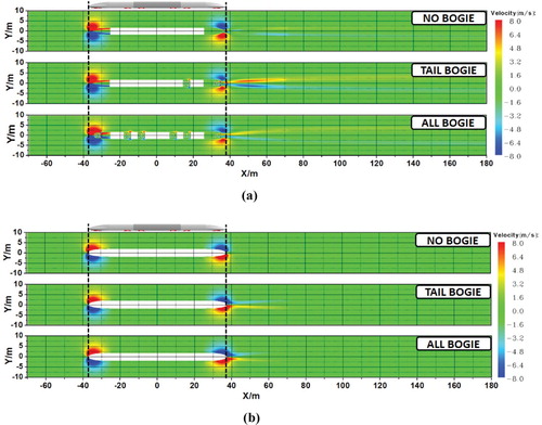
Figure 13 shows the distribution of V_y at different heights for the three simplification models. The absolute value of V_y at the leading and trailing nose is almost the same at the same height. Compared to V_y-0.2, V_y-1.4 keeps the same tendency as well as the magnitude. The bogies show little effect on V_y around the train model. As seen in Figure 15, V_y-0.2 only increases in the wake region. However, the increment is rather smaller than the value around the leading and trailing nose.

Figure 13. Distribution of V_y at different heights: (a) H=0.2 m; (b)H=1.4 m.

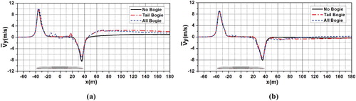
Table 3 shows the maximum values of the slipstream for different simplification models. At different heights, the maximum value of V_y keeps very close. However, V_x drops rapidly when the probe gets higher. At the height of 0.2 m, the values of the slipstream for SP2 and SP3 are very close while the value for SP1 is quite smaller. At the height of 1.4 m, the value of V_y is about twice compared to that of V_x. At the meantime, the value of SP3 is a little greater than that of SP1 and SP2. Comparing all the numerical results and taking the computational cost and accuracy into consideration, SP2 could be chosen as the basic simplification model when performing the slipstream optimization.

Table 3. Maximum values of the slipstream for different simplification models.

Height	Simplification models	Vx(m/s)	Vy(m/s)
0.2 m	SP1	7.9	9.8
	SP2	10.2	9.8
	SP3	10.3	10.2
1.4 m	SP1	4.2	9.0
	SP2	4.2	9.0
	SP3	4.4	9.3

5. Surrogate model

5.1. Sampling method

In this paper, the parameters such as the size requirements of the equipment and structure space in the streamlined area of the Chinese high-speed trains, the vehicle limit requirements, and the length value of the 350 km/h high-speed train head are used as space constraints. Taking the current size of these variables as the baseline, the design space could be determined as Table 4. In order to facilitate analysis, the average value of the design space for each design variable is exactly the value of the baseline. The Latin Hypercube method based on the max-min principle is adopted to obtain the initial sampling points in the design space. 50 sampling points are generated, in which 46 points are chosen as initial training points while the rest 4 points are taken as test points. Since multiple points are added during the construction of surrogate models, the final number of training points is greater than 46, which will be illustrated in the following sections.

Table 4. Design space.

Design variables	Design space	Design variables	Design space	Design variables	Design space
L	[10.0,15.0]	$A_{11}$	[0.2,1.0]	$a_{b1}$	[0.5,2.0]
H	[3.2,3.8]	$A_{21}$	[0.2,0.5]	$a_{b2}$	[1.0,2.0]
c	[3.2,3.6]	$a_{k1}$	[0.5,1.5]	$D_h$	[−20.0,0.0]
r	[4.0,8.0]	$a_{k2}$	[0.5,1.5]	$W_h$	[0.0,25.0]

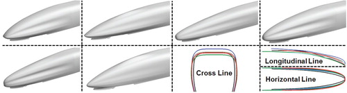
Figure 14 shows the streamlined shapes of 6 randomly selected points and their cross-sectional profiles, longitudinal profiles and horizontal profiles. It could be seen that all the six streamlines own smooth surfaces and distinct clearly from each other. With use of the parametrization methods proposed in the present paper, different types of streamlines could be obtained. The generated streamline could be broad and wide, could be tall and thin, and could also be fusiform. Within the given design space, all kinds of streamlined shapes could be obtained, indicating that the design space used in the present paper is reasonable enough for shape optimization.

Figure 14. Streamlined shapes of 6 randomly selected points and their cross-sectional profiles, longitudinal profiles and horizontal profiles.

5.2. Design objectives

Several design objectives should be considered in practical engineering such as the slipstream, aerodynamic drag, aerodynamic lift, pressure waves, micro pressure waves and aerodynamic noise. In the meantime, some geometric constraints such as the volume of the driving cab which could also affect the assembling space should be taken into consideration as well. In the present paper, the influence of geometric shape of high-speed trains on slipstream is mainly studied. To ensure the optimization results useful for engineering application and obtain the relationships between design variables and slipstream that meet the requirement of aerodynamic performance and geometric constraints, the design objectives are the variables related to the slipstream, the aerodynamic drag of the whole train, C_d, is taken as the constraint related to aerodynamic performance while the volume of the driving cab, V_ol, is taken as the geometric constraint.

The magnitude of slipstream is closely related to the position of the probes. When taking the slipstream as the optimization objective, due to the wide scattering of the magnitude of the slipstream at different positions, the optimization could not be performed if the slipstream of all places is taken into consideration. To ensure the reasonability of the optimization objectives, the engineering standard is fully considered, and the velocity components of the slipstream at standard heights are chosen to be the design objectives.

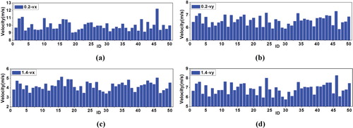
The sampling points in the design space could give a glimpse on the variation of geometric shapes of high-speed trains, and the slipstream of the sampling points could also exhibit its relationship with the geometric shapes. As a result, reasonable design objectives could be determined by analyzing the slipstream of the sampling points. Figure 15 shows the maximum value of V_x and V_y at two standard heights. It could be observed that V_x-0.2 is obviously larger than the others. The distribution of V_x-1.4 is very close to that of V_y at two standard heights. According to TSI 1302–2014 (TSI, 1302, 2014), the maximum values at the standard heights are regulated, which means the maximum value of the slipstream is a main threat to trackside buildings and workers. Considering the width of the train affects directly the slipstream at the height of 1.4 m and V_y-1.4 is greater than V_x-1.4, the maximum value of V_x-0.2 and V_y-1.4 are chosen as the design objectives.

Figure 15. Maximum value of V_x and V_y at two standard heights for all the training samples: (a) V_x-0.2; (b) V_y-0.2; (c) V_x-1.4;(d) V_y-1.4.

5.3. ϵ-TSVR model

Based on the structural risk minimization principle, Support Vector Machine (SVM) algorithm (Peng, 2010), benefits greatly from its ability in generalization and solving nonlinear and high-dimensional problems. SVM algorithm can be divided into two kinds: classification algorithm and regression algorithm, in which, SVM regression algorithm (Support Vector Regression, SVR) has been used widely in engineering (Yao et al., 2016). SVR could also be divided into several kinds, and the ϵ-TSVR(ϵ-twin support vector regression, ϵ-TSVR) proposed by Shao et al. (2013) has been adopted in the present paper. Compared to standard SVR algorithm and TSVR algorithm, ϵ-TSVR owns higher prediction accuracy and less training time. With use of this algorithm, Yao et al. (2016) performed aerodynamic shape optimization of high-speed trains and validated its practicability. For nonlinear regression problem, the original problem of ϵ-TSVR could be expressed as (14) and (15): (14) $\begin{array}{rl}\underset{u_1,b_1,\xi }{min}& \frac{1}{2}{c}_3({\mathit{u}}_1^{\text{T}}{\mathit{u}}_1+b_1^2)+\frac{1}{2}{\mathit{\xi }}^T{\mathit{\xi }}^{\ast }+c_1{\mathit{e}}^T\mathit{\xi },\\ \text{s}.\text{t}.& \mathit{Y}-(K(\mathit{A},{\mathit{A}}^T){\mathit{u}}_1+\mathit{e}{b}_1\ge -{\epsilon }_1\mathit{e}-\mathit{\xi },\mathit{\xi }\ge 0,\\ & \mathit{Y}-(K(\mathit{A},{\mathit{A}}^T){\mathit{u}}_1+\mathit{e}{b}_1={\mathit{\xi }}^{\ast }\end{array}$(14) (15) $\begin{array}{rl}\underset{u_2,b_2,\eta }{min}& \frac{1}{2}{c}_4({\mathit{u}}_2^T{\mathit{u}}_2+b_2^2)+\frac{1}{2}{\mathit{\eta }}^T{\mathit{\eta }}^{\ast }+c_2{\mathit{e}}^T\mathit{\eta },\\ \text{s}.\text{t}.& (\mathit{K}(\mathit{A},{\mathit{A}}^T){\mathit{u}}_1+\mathit{e}{b}_1)-\mathit{Y}\ge -{\epsilon }_2\mathit{e}-\mathit{\eta },\mathit{\eta }\ge 0,\\ & (\mathit{K}(\mathit{A},{\mathit{A}}^T){\mathit{u}}_2+\mathit{e}{b}_2)-\mathit{Y}={\mathit{\eta }}^{\ast }\end{array}$(15)

In which, $c_1$, $c_2$, $c_3$, $c_4$, ${\epsilon }_1$ and ${\epsilon }_2$ are variables bigger than zero. ${\mathit{u}}_1$and ${\mathit{u}}_2$ are vectors.$b_1$ and $b_2$ are coefficients. $\mathit{\xi }$, ${\mathit{\xi }}^{\ast }$, $\mathit{\eta }$ and ${\mathit{\eta }}^{\ast }$ are relaxation vectors. $\mathit{K}(\mathit{A},{\mathit{A}}^T)$ is the kernel function, and the Gaussian function is chosen as the kernel function in the present paper, just as (16) shows, in which $\sigma$ is the width factor. (16) $exp\left(-\frac{1}{2{\sigma }^2}{||\mathit{x}-{\mathit{x}}_i||}^2\right)$(16)

For the m-dimensional problem with n training samples, the corresponding $\mathit{A}$ is an m×n matrix where $A_i$ is the i-th training sample, $\mathit{Y}=(y_1,y_2,\dots ,y_m)$ is the corresponding response value and $\mathit{e}$ is the unit vector. By constructing Lagrangian function, the dual problem of (14) and (15) could be obtained with use of the Karush-Kuhn-Tucker complementary condition, just as (17) and (18) show. The detailed deduction process could be referred to in literature (Yao et al., 2016). (17) $\begin{array}{rl}\underset{\mathit{\alpha }}{max}& -\frac{1}{2}{\mathit{\alpha }}^T\mathit{H}({\mathit{H}}^T\mathit{H}+c_3\mathit{I}{)}^{-1}{\mathit{H}}^T{\mathit{\alpha }}^T-({\mathit{e}}^T{\epsilon }_1+{\mathit{Y}}^T)\mathit{\alpha }\\ & +{\mathit{Y}}^T\mathit{H}({\mathit{H}}^T\mathit{H}+c_3\mathit{I}{)}^{-1}{\mathit{H}}^T\mathit{\alpha }\\ \text{s}.\text{t}.& \mathbf{0}\le \mathit{\alpha }\le c_1\mathit{e}.\end{array}$(17) (18) $\begin{array}{rl}\underset{\mathit{\gamma }}{max}& -\frac{1}{2}{\mathit{\gamma }}^T\mathit{H}({\mathit{H}}^T\mathit{H}+c_4\mathit{I}{)}^{-1}{\mathit{H}}^T{\mathit{\gamma }}^T-({\mathit{Y}}^T-{\mathit{e}}^T{\epsilon }_2)\mathit{\gamma }\\ & -{\mathit{Y}}^T\mathit{H}({\mathit{H}}^T\mathit{H}+c_4\mathit{I}{)}^{-1}{\mathit{H}}^T\mathit{\gamma }\\ \text{s}.\text{t}.& \mathbf{0}\le \mathit{\gamma }\le c_2\mathit{e}.\end{array}$(18) where, (19) $\mathit{H}=[\mathit{K}(\mathit{A},{\mathit{A}}^T)\mathit{e}]$(19) (20) ${\mathit{v}}_1=({\mathit{H}}^T\mathit{H}+c_3\mathit{I}{)}^{-1}{\mathit{H}}^T(\mathit{Y}-\mathit{\alpha })$(20) (21) ${\mathit{v}}_2=({\mathit{H}}^T\mathit{H}+c_4\mathit{I}{)}^{-1}{\mathit{H}}^T(\mathit{Y}+\mathit{\gamma })$(21) where ${\mathit{v}}_1=[{\mathit{u}}_1^T{b}_1{]}^T$, ${\mathit{v}}_2=[{\mathit{u}}_2^T{b}_2{]}^T$. The values of ${\mathit{u}}_1$, ${\mathit{u}}_2$, ${\mathit{b}}_1$ and ${\mathit{b}}_2$ could be obtained by solving (11) and (12). Then the prediction value of ϵ-TSVR could be obtained by (22) (22) $\begin{array}{rl}f(\mathit{x})& =\frac{1}{2}(f_1(\mathit{x})+f_2(\mathit{x}))\\ & =\frac{1}{2}({\mathit{u}}_1^T+{\mathit{u}}_2^T)\mathit{K}(\mathit{A},\mathit{x})+\frac{1}{2}(b_1+b_2)\end{array}$(22)

When training samples are determined, the free coefficients $c_1$, $c_2$, $c_3$, $c_4$, ${\epsilon }_1$, ${\epsilon }_2$ and $\sigma$in ϵ-TSVR model could affect efficiently on the generalization ability of the model. However, there is no theoretical basis to strictly calculate these coefficients till now. In the present paper, these coefficients are determined by cross validation method and PSO algorithm. On the condition that the prediction accuracy of the ϵ-TSVR model isn’t reduced, to simplify this problem and improve the training efficiency of the ϵ-TSVR model, we assume $c_1=c_2$ and $c_3=c_4$. c₃ and c₄ have the same effect in the dual expressions, so are c₁ and c₂. It won’t reduce the prediction accuracy of the model to make c₃ equals c₄ and c₁ equals c₂. On the contrary, the number of free coefficients is reduced. As a result, there are five free coefficients needed to be determined in total. For a set of given free coefficients, the quadratic programing problem (17) and (18) needs to be solved twice. In order to improve the training efficiency, the overrelaxation iteration technique has been introduced by Shao et al. (2013), which is also adopted in the present paper.

The construction process of ϵ-TSVR model is also the determination process of free coefficients. For a single ϵ-TSVR model, the determination of the five free coefficients could be performed by the following steps:

1. For the given training set, divide the training samples into l groups randomly. Make sure the number of training samples in each group is the same, which is 2 in the present study.

2. Determine the initial coefficients in PSO algorithm, such as the population and the iteration steps. The number of particles and iteration steps are crucial to the optimization efficiency, which should not be too big or too small. The population in PSO in the present study is 35 and the number of iteration steps is 300.

3. Sequentially select each group as the test samples, and use the other training samples to construct a sub SVR model. Then obtain the prediction error $\mathrm{\%}RMS{E}_i$ of the test samples. The fitness in PSO algorithm takes the form as (23) (23) $\text{fit}=\frac{1}{l}\sum _{i=1}^l\mathrm{\%}RMS{E}_i$(23) where l is the number of groups, and $\mathrm{\%}RMS{E}_i$ is the i-th prediction error of the test samples, which could be expressed as (24): (24) $\mathrm{\%}RMSE=100\sqrt{\frac{1}{n_s}\sum _{i=1}^{n_s}{(y_i-y_i^{(p)})}^2}/\frac{1}{n_s}\sum _{i=1}^{n_s}{y}_i$(24) where $y_i$ is the real value, $y_i^{(p)}$ is value predicted by SVR and $n_s$ is the number of test samples.

4. Obtain the optimal values of free coefficients after iterations. When using SVR model, take the average value of each sub SVR model as the final prediction value.

The ϵ-TSVR models should be built for each design objectives and constraints. There are two design objectives and two constraints, so that four ϵ-TSVR models should be constructed. The initial samples for each ϵ-TSVR are the same. Since the relationships between design variables and design objectives or constraints in the design space are different, the variations of the design objectives or constraints are quite different from each other. As a result, the prediction accuracy of ϵ-TSVR models varies from each other on the base of same initial samples. In the present paper, the final ϵ-TSVR model should assure the averaged prediction error no bigger than 5% and the maximum prediction error no bigger than 10%.

Figure 16 shows the construction process for ϵ-TSVR models. If the prediction accuracy doesn’t meet the requirement, additional sample points should be added to the training set. There are two steps to add these points:

1. For a single-objective ϵ-TSVR model, add the test samples into the training set to restart the construction process if the prediction accuracy doesn’t meet the requirement. Further test samples are selected randomly among the samples in the design space. Repeat the process until the prediction accuracy meets the requirement. In the present paper, the number of test points is 4.

2. The Pareto set could be obtained after the final ϵ-TSVR model set have been constructed. Several points from the Pareto set are taken as test samples. If the prediction accuracy doesn’t meet the requirement, these points are added into the initial training set to rebuild the ϵ-TSVR models. Otherwise, the Pareto set will work as the final optimization results. 6 points from the Pareto set are taken from the Pareto set.

Figure 16. Construction process for ϵ-TSVR models.

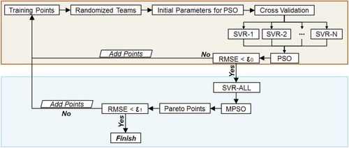
During the adding points process, only the ϵ-TSVR model which doesn’t meet the accuracy requirement needs to add more points to the training set. For those ϵ-TSVR models that meet the accuracy requirement, there’s no need to add points. As a result, the number of final training points differs from each other when all the ϵ-TSVR models is precise enough.

Table 5 gives the prediction errors of the ϵ-TSVR models on the base of initial training points. The values of the slipstream and aerodynamic drag obtained from DDES method are taken as the exact values. The exact value of the volume of the driving cab could be obtained by geometric integration. It could be observed that the ϵ-TSVR model of V_x-0.2 own the biggest prediction error, while the error of the ϵ-TSVR model of V_ol is the smallest. All the four ϵ-TSVR models meet the accuracy requirement. As a result, there’s no need to add more points for the first step.

Table 5. Prediction errors of the ϵ-TSVR models on the base of initial training points.

Test samples	Vx-0.2		Vy-1.4		Cd		Vol
Evaluation Methods	DDES	ϵ-TSVR	DDES	ϵ-TSVR	DDES	ϵ-TSVR	REAL	ϵ-TSVR
T1	9.35	9.64	6.91	6.77	0.220	0.217	0.0323	0.0324
T2	10.04	9.86	7.67	7.80	0.229	0.232	0.0311	0.0312
T3	9.51	10.02	7.73	7.75	0.225	0.227	0.0337	0.0336
T4	9.97	9.64	8.80	8.50	0.241	0.239	0.0234	0.0236
Average Error	3.59%		2.30%		1.11%		0.44%
Maximum Error	5.36%		3.45%		1.36%		0.85%

As for adding points in the second step, we need to obtain the Pareto set with use of the ϵ-TSVR model set and multi-objective PSO. This process will be introduced in detail in section 6.2.

6. Results and discussions

6.1. Multi-objective particle swarm optimization method

The PSO algorithm was proposed in 1995 by Kennedy and Eberhart (1995). This algorithm is simple in principle, easy to implement and has strong global optimization ability. Moore and Chapman (1999) used the PSO algorithm in 1999 for the first time to solve the multi-objective problem. Afterwards, several kinds of multi-objective PSO algorithm has been proposed. Based on the non-inferior classification idea, Li (2003) developed the NSPSO method by introducing the concept of niche technology and crowding distance into the original PSO algorithm. Results revealed that NSPSO owned stronger optimization ability than NSGA-II. The external file was introduced into the NSPSO method by Yao et al. (2015, 2016). The niche count and crowding distance technique are also used to judge the performance of the particles in the external file. The particle with the best performance is chosen to be the global best particle. Consequently, a new MPSO method was proposed. This method is also adopted in the present paper. Some coefficients used in MPSO are listed as follows: the number of the population is 200 and the number of iteration steps is 10000. The acceleration factor is 2. The inertia factor gradually varies from 1.2–0.4 during the iteration. The maximum flying speed is 0.3.

In order to study the influence of design variables on the slipstream, aerodynamic drag and volume of the driving cab (which is represented by the volume of the streamline), two design objectives are defined while the other two and the length of the streamline work as constraint objectives. The drag coefficient of the whole train (0.231) and volume of driving cab for the original model (0.0278) are taken as the constraints. 90% of the values of V_x-0.2 (10.36) and V_x-1.4 (7.94) of the original model are taken as the limit of the constraints. Six groups of fitness functions are defined to get six Pareto set P_i, i=1,2, … ,6.

The fitness functions for P₁, P₂, P₃ and P₄ take the form as: (25) $\begin{array}{rl}{f}_1& =f_1+{\varphi }_1\end{array}$(25) (26) $\begin{array}{rl}{f}_2& =f_2+{\varphi }_2\end{array}$(26)

For P₁, ${\varphi }_1$ and ${\varphi }_2$ are 0.

For P₂, ${\varphi }_1$ and ${\varphi }_2$ take the form as: (27) $\begin{array}{rl}{\varphi }_1& =2|min(0,0.231-f_3){|}^{0.1}+2|min(0,f_4-0.0278){|}^{0.1}\end{array}$(27) (28) $\begin{array}{rl}{\varphi }_2& =2|min(0,0.231-f_3){|}^{0.1}+2|min(0,f_4-0.0278){|}^{0.1}\end{array}$(28)

For P₃, ${\varphi }_1$ and ${\varphi }_2$ are 0 and the design variable L is set to be 12.5 m.

For P₄, ${\varphi }_1$ and ${\varphi }_2$ take the form as: (29) $\begin{array}{rl}{\varphi }_1& =2|min(0,0.231-f_3){|}^{0.1}\\ & +2|min(0,f_4-0.0278){|}^{0.1}\end{array}$(29) (30) $\begin{array}{rl}{\varphi }_2& =2|min(0,0.231-f_3){|}^{0.1}\\ & +2|min(0,f_4-0.0278){|}^{0.1}\end{array}$(30)

The design variable L is set as 12.5 m.

The fitness functions of P₅ and P₆ take the form as: (31) $f_3=f_3+{\varphi }_3$(31) (32) $f_4=f_4+{\varphi }_4$(32)

For P₅, ${\varphi }_1$ and ${\varphi }_2$ are 0.

For P₆, ${\varphi }_1$ and ${\varphi }_2$ take the form as: (33) ${\varphi }_3=2|min(0,9.32-f_1){|}^2+2|min(0,7.15-f_2){|}^2$(33) (34) ${\varphi }_4=2|min(0,9.32-f_1){|}^2-2|min(0,7.15-f_2){|}^2$(34)

In which, $f_1$ is the maximum value of V_x-0.2, $f_2$ is the maximum value of V_y-1.4, $f_3$ is the aerodynamic drag of the whole train, and $f_4$ is the volume of the driving cab.

6.2. Pareto set

The prediction accuracy of the ϵ-TSVR models determines the final optimization results. Based on the ϵ-TSVR models built in section 5.3, six Pareto sets could be obtained, as shown in Figure 15. One test point P_0i (i=1,2, … ,6) from each Pareto set is taken to perform numerical analysis, and the numerical results are given in Table 6. It could be seen that the averaged and maximum error for V_x-0.2 are 9.61% and 13.31% respectively, which don’t meet the accuracy requirement. Meanwhile, the averaged and maximum error for V_y-1.4 are 7.85% and 15.89% respectively, which don’t meet the accuracy requirement either. As a result, all these six points are added to the training set of V_x-0.2 and V_y-1.4 to rebuild the corresponding ϵ-TSVR model. Based on the rebuilt ϵ-TSVR models, six new Pareto sets are obtained. Repeating the validation process, one test point P_1i (i=1,2, … ,6) from each Pareto set is taken to perform DDES analysis, and the results are also shown in Table 6. It could be seen that the averaged and maximum error of each design objective all meet the accuracy requirement for the second round. As a result, the new six Pareto sets are exactly the final Pareto set, as shown in Figure 17.

Table 6. Comparison of the test samples in the Pareto set.

	Test samples	Vx-0.2		Vy-1.4		Cd		Vol
Adding point times	Evaluation ways	DDES	ϵ-TSVR	DDES	ϵ-TSVR	DDES	ϵ-TSVR	REAL	ϵ-TSVR
0	P01	9.65	8.51	5.71	5.29	0.199	0.194	0.0268	0.0271
	P02	9.75	8.76	5.62	5.18	0.199	0.196	0.0273	0.0278
	P03	9.94	8.62	6.47	6.14	0.206	0.203	0.0220	0.0214
	P04	9.46	9.01	7.41	7.36	0.226	0.228	0.0277	0.0278
	P05	9.27	9.53	6.84	6.80	0.213	0.210	0.0322	0.0327
	P06	9.42	8.53	6.39	5.38	0.199	0.193	0.0270	0.0273
	Average Error	9.61%		7.85%		3.28%		1.52%
	Maximum Error	13.31%		15.89%		2.86%		2.81%
1	P11	9.16	8.73	5.88	5.79	0.201	0.198	0.0281	0.0287
	P12	9.61	9.33	5.68	5.47	0.200	0.197	0.0274	0.0280
	P13	9.54	9.86	6.49	6.50	0.208	0.210	0.0231	0.0231
	P14	9.06	8.54	7.49	7.51	0.226	0.228	0.0280	0.0279
	P15	9.88	10.44	8.42	8.24	0.234	0.234	0.0397	0.0377
	P16	9.06	8.47	6.66	6.74	0.216	0.212	0.0331	0.0323
	Average Error	4.96%		1.82%		1.85%		3.16%
	Maximum Error	6.51%		3.70%		1.24%		5.04%

Figure 17. Distribution of six Pareto sets: (a) P₁; (b) P₂; (c) P₃; (d) P₄; (e) P₅; (f) P_6.

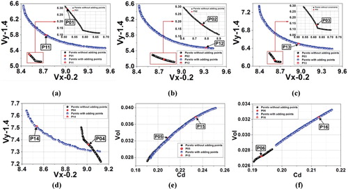
Due to the accuracy difference of ϵ-TSVR models, the distribution of Pareto set varies dramatically before and after adding points except for P₅, as shown in Figure 17. Before adding points, the prediction accuracy of ϵ-TSVR models around the optimal solution region is relatively poor, resulting in unreasonable optimal points gathering in a limited region. After adding points, the distribution of Pareto set spreads wider. The ϵ-TSVR models corresponding to P₅ keep unchanged since only two times of optimization have been carried out before and after adding points. As seen in Figure 17(e), the results of two optimizations coincide basically, indicating that the optimization algorithm owns high accuracy and the optimization results are very robust.

As indicated by the distribution of P₁, P₂, P₃ and P₄, different fitness functions could lead to totally different Pareto set. The distribution of P1 is very similar to that of P3, but the distribution of V_y-1.4 is much wider, indicating that the constraint of L influences greatly on V_y-1.4. The influence of ${\varphi }_1$and ${\varphi }_2$ on $f_1$ and $f_2$ is very little. However, after adding the constraints of ${\varphi }_3$ and ${\varphi }_4$, the distribution of P₆ gets narrower compared to P₅. The minimum optimal values of $f_3$ and $f_4$ get increased, while the maximum optimal values get decreased.

Due to the influence of ground effect, the flow near the ground is more easily to be disturbed by the variation of streamlined shape, and V_x-0.2 exhibits stronger nonlinear relationship with the design variables. Consequently, the construction of corresponding ϵ-TSVR model is more difficult. Overall, the prediction error of V_x-0.2 is much bigger than that of the other three objectives, just as Table 6 shows. After adding points for the first time, the accuracy of the ϵ-TSVR model of V_x-0.2 improves greatly. The averaged error is near 5% while the maximum error is quite lower than 10%. Meanwhile, the averaged and maximum error of V_y-1.4 are both greatly reduced too, indicating that adding points around the optimal solution region could effectively improve the prediction accuracy. The ϵ-TSVR models corresponding to C_d and V_ol don’t need to add points since the initial models have already met the accuracy requirement. As a result, before and after adding points, essentially, two times of optimization have been performed for these two models. Since the averaged and maximum error of these two ϵ-TSVR models both meet the accuracy requirement, no more detailed accuracy validation will be performed in the present paper.

Taking P_1i (i=1,2, … ,6) in Table 6 as the optimal shapes, the design variables corresponding to each sample point are shown in Table 7. It could be seen that the variable L always takes the maximum value in the design space. Limited by the constraints, L takes the value of 12.5 m for P₁₃ and P₁₄, indicating that long streamline could aid in reducing the values of design objectives. Except for P₁₅, the values of $c$ and $a_{b2}$ of the other designs take the minimum value in the design space, while the value of $a_{k2}$ takes the maximum value. These specific values could lead to the reduction of the width of the train, indicating that smaller width of the train could lead to smaller aerodynamic drag and weaker slipstream. The values of other design variables vary greatly from each other, indicating the geometric shapes of the optimal designs distinct obviously from each other.

Table 7. Design variables corresponding to each sample point.

Design points	L	H	c	r	$A_{11}$	$a_{k1}$	$a_{b1}$	$A_{21}$	$a_{k2}$	$a_{b2}$	$D_h$	$W_h$
P11	15.0	3.200	3.200	6.275	0.523	0.627	1.325	0.388	1.500	1.000	−20.000	16.035
P12	15.0	3.200	3.200	7.479	0.668	0.968	0.929	0.304	1.500	1.000	−17.516	2.204
P13	12.5	3.200	3.200	7.558	0.200	0.749	1.012	0.379	1.500	1.000	−20.000	7.500
P14	12.5	3.800	3.200	6.177	0.200	0.653	1.726	0.423	1.500	1.000	−18.393	15.563
P15	15.0	3.800	3.351	4.000	0.200	0.910	1.379	0.483	0.556	1.814	−7.643	24.373
P16	15.0	3.649	3.200	5.497	0.200	0.500	2.000	0.500	1.500	1.000	−20.000	25.000

Figure 18 shows the streamlined shapes corresponding to the above sample points. It could be observed that the streamlined shapes all own deeper drainage along the lateral sides except P₁₅. This kind of design could induce the incoming flow passing along the drainage and decrease the propagation in transverse direction. P₁₅ is obtained considering C_d and V_ol only, indicating that the design of drainage has little effect on C_d. Moreover, the shallower the drainage is, the bigger V_ol is. From the topologic view, P₁₁ and P₁₂ belong to fusiform streamlines, while P₁₃, P₁₄, P₁₅ and P₁₆ are tall and thin, indicating that the relationships between V_ol and V_x-0.2, V_y-1.4 and C_d are negative related. The bigger V_ol is, the harder to reduce V_x-0.2, V_y-1.4 and C_d. If the constraint of V_ol is much stricter, a better way to reduce V_x-0.2, V_y-1.4 and C_d is to increase the projection area of longitudinal section and reduce the projection area of horizontal section.

Figure 18. Streamlined shapes corresponding to the above sample points.

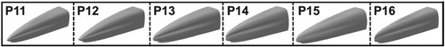
The values of design objectives corresponding to each design point are shown in Table 8. Compared to the initial shape, the values of design objectives are all reduced in a certain extent. For P₁₁, V_ol is very close to that of the initial shape. However, V_x-0.2, V_x-1.4, V_y-0.2, V_y-1.4 and C_d are reduced by 11.6%, 33.9%, 24.7%, 25.9% and 13.0% respectively. Similarly, focusing on P₁₂, it could be found that V_ol is a little smaller than that of the initial shape. Most of the other objectives are reduced prominently except that V_x-0.2 has been increased by 4.9%. The length of the streamline of P₁₄ is 12.5 m, and V_ol of P₁₄ is also very close to that of the initial shape. As for the other objectives, V_x-0.2, V_y-0.2 and V_y-1.4 are reduced by 12.5%, 6.3% and 5.7% respectively. It could be deduced that if the length of the streamline and the volume of the driving cab have already been determined, the slipstream could be reduced greatly by shortening the width and increasing the height of the train body. It also gets little influence on the aerodynamic drag. Comparing the objectives of P₁₅ and P₁₆ with the initial shape, we could find that the slipstream and drag of the train could be greatly reduced together with increasing the volume of the driving cab by controlling the length of the streamline. In China, there is a high demand for double-deck high-speed trains, whose height of the train body is obviously higher than ordinary trains. Following the study in this section, it could be recommended that the streamlined shape of double-deck train could be designed to be narrower and taller.

Table 8. Values of design objectives corresponding to each design point.

Design point	Vx-0.2	Vx-1.4	Vy-0.2	Vy-1.4	Cd	Vol
Initial shape	10.36	4.40	8.47	7.94	0.231	0.0278
P11	9.16	2.91	6.38	5.88	0.201	0.0281
P12	9.61	2.83	6.22	5.68	0.200	0.0274
P13	9.54	3.17	7.09	6.49	0.208	0.0231
P14	9.06	3.78	7.94	7.49	0.226	0.0280
P15	9.88	4.11	8.89	8.42	0.234	0.0397
P16	9.06	3.35	7.11	6.66	0.216	0.0331

P₁₁ is chosen as the final optimal shape to be compared with the initial shape. Figure 19 shows the contours of V_x and V_y at different heights before and after optimization. At the height of 0.2 m, the high velocity region near the leading nose is greatly reduced after optimization. Moreover, the high velocity region in the wake tends to gather in the center line of the train. This kind of flow distribution could greatly reduce the value of V_x and V_y in the region near the leading nose and in the wake. At the height of 1.4 m, due to the increase of the length of the streamline and the decrease of the width of the train, the regions where V_y varies severely around the leading and trailing nose get lengthened in the streamwise direction and shrunk in transverse direction. Meanwhile, the maximum value of V_y gets reduced, which could help to reduce the local slipstream. Because of the weakening of flow separation in the wake region after optimization, V_y gets reduced obviously in the wake region. As a result, the deformation of the streamline shape could not only influence the slipstream around the train body, but also affect the slipstream in the wake far away from the trailing nose.

Figure 19. Contours of V_x and V_y at different heights before and after optimization: (a) V_x; (b) V_y.

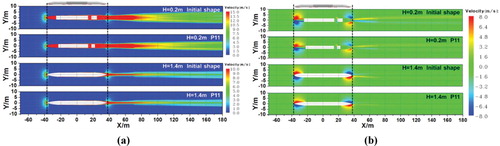
Figure 20 shows the iso-surface of Q at t = 2s before and after optimization. Complicated vortex structures could be seen separated from the trailing nose. Two sets of anti-symmetrical vortex structures detach from lateral sides of the trailing nose. As propagating downward, the vortex cores grow bigger and bigger. Although the intensity of the vortex structures tends to decrease, the influenced region in length and width directions grows larger. Compared to the initial shape, the length of the streamline increases, and the width of the train grows smaller. Consequently, the variation ratio of the cross section of the streamline tends to be more complanate, which could lead to weak separation in the wake region. The anti-symmetrical vortex structures get closer to the center of the train (y = 0). In the wake region far away from the trailing nose, the intensity of the vortex structures drops greatly, resulting in weaker influence in the lateral sides of the train. Such change of flow structures after optimization could aid in reducing the slipstream in the wake region.

Figure 20. Iso-surface of Q at t=2s before and after optimization (t=2s, Q=5, shaded by pressure).

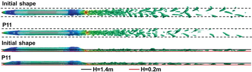
Figure 21 shows the time-averaged value of V_x at different heights before and after optimization. The absolute values of V_x around the leading and trailing nose get reduced obviously at the heights of 0.2 and 1.4 m. The distribution of V_x in the wake region tends to be more complanate after optimization, and the peak value of V_x also gets decreased. At the height of 0.2 m, the peak value of V_x is much more far away from the trailing nose after optimization. At the height of 1.4 m, the peak value of V_x is much smaller than that around the train body, indicating that the change of streamlined shape could greatly affect the wake flow. Results also reveal that the most reduction region of the slipstream at different heights could be affected by the topology of streamlined shape.

Figure 21. Time-averaged V_x at different heights before and after optimization: (a) H=0.2 m; (b) H=1.4 m.

Figure 22 shows the time-averaged value of V_y at different heights before and after optimization. It could be seen that the distribution profiles of V_y keep similar before and after optimization. V_y is very close to zero around the middle carriage and in the wake region. The obvious difference is the maximum value. The peak values of V_y around the leading and trailing car decrease dramatically after optimization. At the height of 0.2 m, V_y also get reduced in the wake region, indicating that the change of streamlined shape could influence both the deformation region and the near ground region in the wake.

Figure 22. Time-averaged V_y at different heights before and after optimization: (a) H=0.2 m; (b) H=1.4m.

6.3. Sensitivity analysis

During the engineering design of high-speed trains, the relationship of key design variables with the objectives could offer directly the design insight. Based on the ϵ-TSVR models, the relationships of 12 design variables and objectives are obtained. The design space of each design variable is normalized into [0, 1] to facilitate the following analysis, as shown in Figure 23. It could be seen that compared to the other three objectives, the relationships between design variables and V_x-0.2 exhibit strong nonlinear relationships. However, due to the relatively large range of the y coordinate, this kind of nonlinear relationship could not be directly seen. Taking H and w_h as examples, the relationships with are depicted in Figure 23(a). As c increases, the value of V_x-0.2 increases too. The design variables, A₂₁ and a_k2, are the two variables that control the horizontal profile of the streamline. When they grow bigger, the value of V_x-0.2 becomes smaller, indicating that the streamline which is tall and thin could benefit in reducing the value of V_x-0.2. Meanwhile, the variable H has little influence on V_x-0.2. The variable L is the key factor that influences V_y-1.4, C_d and V_ol. The bigger L is, the smaller V_y-1.4 and C_d are. Bigger V_ol indicates that the streamline is very longer, which could help to improve the aerodynamic performance. However, from the engineering view, although long streamline could lead to larger driving cab, the passengers’ carriage could be shortened, and finally the number of passengers in the first carriage could be decreased. The variable H is the second important factor that affects V_y-1.4, C_d and V_ol. As H grows bigger, the values of V_y-1.4, C_d and V_ol also grow larger, indicating higher train body could lead to bad aerodynamic performance. As a result, consideration should be taken synthetically between the influence of height of the train body on aerodynamic performance and the volume of the driving cab. The influence of other design variables on objectives is different and gets different relationships, the quantitative results are shown in Table 9.

Figure 23. Relationships of 12 design variables and objectives: (a) V_x-0.2;(b) V_y-1.4; (c) C_d; (d) V_ol.

Table 9. Values of sensitivity analysis of the design variables on design objectives.

Design variables	Vx-0.2	Vy-1.4	Cd	Vol
L	−0.2387	−2.2363	−0.0267	0.0116
H	0.1183	0.9537	0.0170	0.0042
$c$	0.7439	0.6416	0.0146	0.0022
$r$	−0.1110	−0.4398	−0.0042	−0.0015
$A_{11}$	0.2739	0.0198	−0.0035	−0.0011
$a_{k1}$	0.2453	−0.1171	−0.0013	−0.0002
$a_{b1}$	−0.1034	0.2154	0.0036	0.0009
$A_{21}$	−0.4838	0.0003	−0.0080	−0.0010
$a_{k2}$	−0.9976	−0.9644	−0.0057	−0.0014
$a_{b2}$	0.5817	0.7053	0.0110	0.0021
$D_h$	0.5113	0.2762	0.0005	0.0004
$W_h$	−0.0477	0.1578	−0.0002	0.0003

In order to better understand the influence of design variables on the objectives, the finite difference method is adopted to perform the sensitivity analysis on each design variable. Positive result indicates that the design variables are positively related to the objectives and vice versa. The bigger the absolute value of the analysis result is, the greater the contribution of design variables is. Table 9 shows the values of sensitivity analysis of the design variables on design objectives. It could be found that except for the width of the train body, the longitudinal and horizontal profiles of the streamline have the greatest influence on V_x-0.2. The depth of the drainage has greater influence on V_x-0.2 compared to the other objectives. The length of the streamline affects greatly on V_y-1.4, C_d and V_ol while has little influence on V_x-0.2. The variable a_k2 controls the curvature of the middle part of the horizontal profile. It is negatively related to the slipstream and aerodynamic drag. The variables that affect the design objectives in the same way could be called isotropic variables. When designing the aerodynamic shape of high-speed trains, it is a better way to optimize on the most important objectives. By varying the isotropic variables, the other objectives could be optimized at the same time. Such variables also include L, H, c, r, a_b2 and D_h. For the variables that affect the design objectives in the opposite ways, they could be called anisotropic variables. The value of anisotropic variables should be well considered to match the different design objectives.

7. Conclusions

The slipstream induced by high-speed trains affects the safety of trackside structures and workers severely, which is a key factor during the aerodynamic design of high-speed trains. Based on the DDES method, ϵ-TSVR models and multi-objective PSO method, multi-objective aerodynamic optimization with certain constraints has been performed, and the influence of aerodynamic shape on the slipstream has been investigated. The main conclusions are as follows:

1. The profile superposition method has been developed to parameterize the cross-section of the train body, and the VMF method has been adopted to parameterize the streamlined shape of the train. 12 variables are designed to control the deformation of the train. As a result, the parametrization of the whole train has been accomplished.

2. Based on the wind tunnel test data, the computational accuracy of the stationary method and moving mesh method with use of DDES method has been validated. On the base of stationary method, the influence of bogies on the slipstream has been analyzed. Results reveal that the trailing bogies have the greatest influence on the slipstream in the wake region.

3. The velocity of the slipstream at standard places, the aerodynamic drag of the whole train model and the volume of the driving cab are taken as design objectives. Four ϵ-TSVR models are constructed for each design objective. Based on different constraints and fitness functions, 6 different Pareto sets are obtained with use of the multi-objective PSO method. 6 samples are chosen from each Pareto set and one of the samples is chosen as the final optimal shape. Compared to the initial shape, the volume of the driving cab keeps almost the same after optimization. However, V_x-0.2, V_x-1.4, V_y-0.2, V_y-1.4 and C_d are reduced by 11.6%, 33.9%, 24.7%, 25.9% and 13.0% respectively.

4. If the volume of the driving cab is constrained, the streamlines which are tall and thin will benefit in reducing the slipstream and aerodynamic drag. The length of the streamline has the greatest influence on aerodynamic performance, while the height and width of the train body are also very important factors. The depth of the drainage owns greater influence on V_x-0.2 compared to its influence on V_y-1.4, C_d and V_ol.

Confined by local experimental conditions and some safety issues, it is very hard to acquire the real vehicle test data about train wind in China. However, it is also a more reliable approach to test the train wind by moving model experiments. The focus of current study is to use optimization methods to reduce the train wind. In order to assure the reliability of the optimization result, the wind tunnel experimental data is utilized to validate the accuracy of numerical algorithms on the condition that no direct real vehicle test data is available. However, this kind of validation has certain limitations, because the surface pressure of the car body and the aerodynamic force of the train cannot directly show the unsteady flow characteristics around the train. In addition, limited by the test conditions, the optimized shape hasn’t been validated by the wind tunnel test or moving model test. Therefore, on the basis of the current work, it is necessary to carry out model test or real vehicle test for the train wind. On the one hand, more reliable test data could be provided for the validation of numerical simulations. On the other hand, the optimization effect of this paper could be verified, and further the reliability of current optimization methods.

Acknowledgments

This work was supported by Advanced Rail Transportation Special Plan in National Key Research and Development Project under 2016YFB1200601-B13, 2016YFB1200602-09 and Youth Innovation Promotion Association CAS. And Computing Facility for the ‘Era’ petascale supercomputer of Computer Network Information Center of Chinese Academy of Sciences is gratefully acknowledged.

Disclosure statement

No potential conflict of interest was reported by the author(s).

Additional information

Funding

This work was supported by Advanced Rail Transportation Special Plan in National Key Research and Development Project under 2016YFB1200601-B13, 2016YFB1200602-09 and Youth Innovation Promotion Association CAS. And Computing Facility for the ‘Era’ petascale supercomputer of Computer Network Information Center of Chinese Academy of Sciences is gratefully acknowledged.

References

- Baker, C. (2010). The flow around high speed trains. Journal of Wind Engineering and Industrial Aerodynamics, 98(6), 277–298. https://doi.org/10.1016/j.jweia.2009.11.002
- Bell, J. R., Burton, D., Thompson, M., Herbst, A., & Sheridan, J. (2014). Wind tunnel analysis of the slipstream and wake of a high-speed train. Journal of Wind Engineering and Industrial Aerodynamics, 134, 122–138. https://doi.org/10.1016/j.jweia.2014.09.004
- Bell, J. R., Burton, D., Thompson, M., Herbst, A., & Sheridan, J. (2017). The effect of tail geometry on the slipstream and unsteady wake structure of high-speed trains. Experimental Thermal and Fluid Science, 83, 215–230. https://doi.org/10.1016/j.expthermflusci.2017.01.014
- Farzaneh-Gord, M., Faramarzi, M., Almadi, M. H., Sadi, M., Shamshirband, S., Mosavi, A., & Chau, K. W. (2019). Numerical simulation of pressure pulsation effects of a snubber in a CNG station for increasing measurement accuracy. Engineering Applications of Computational Fluid Mechanics, 13(1), 642–663. https://doi.org/10.1080/19942060.2019.1624197
- Gao, G., Li, F., He, K., Wang, J., Zhang, J., & Miao, X. (2019). Investigation of bogie positions on the aerodynamic drag and near wake structure of a high-speed train. Journal of Wind Engineering and Industrial Aerodynamics, 185, 41–53. https://doi.org/10.1016/j.jweia.2018.10.012
- Ghalandari, M., Shamsirband, S. M., Mosavi, A., & Chau, K. W. (2019). Flutter speed estimation using presented differential quadrature method formulation. Engineering Applications of Computational Fluid Mechanics, 13(1), 804–810. https://doi.org/10.1080/19942060.2019.1627676
- Guo, D., Shang, K., Zhang, Y., Yang, G., & Sun, Z. (2016). Influence of affiliated components and train length on the train wind. Acta Mechanica Sinica, 32(2), 191–205. https://doi.org/10.1007/s10409-015-0553-z
- Hemida, H., & Krajnovic, S. (2010). LES study of the influence of the nose shape and yaw angles on flow structures around trains. Journal of Wind Engineering and Industrial Aerodynamics, 98(1), 34–46. https://doi.org/10.1016/j.jweia.2009.08.012
- Kennedy, J., & Eberhart, R. C. (1995). Particle swarm optimization. In: Proceeding of the 1995 IEEE international conference on neural network, Perth, 1942-1948.
- Ku, Y. C., Park, H., Kwak, M. H., & Lee, D. H. (2010). Multi-objective optimization of high-speed train nose shape using the vehicle modeling function. In: 48th AIAA aerospace sciences meeting, Orlando, USA.
- Ku, Y. C., Rho, J. H., Yun, S. H., Kwak, M. H., Kim, K. H., Kwon, H. B., & Lee, D. H. (2010). Optimal cross-sectional area distribution of a high-speed train nose to minimize the tunnel micro-pressure wave. Structural and Multidisciplinary Optimization, 42(6), 965–976. https://doi.org/10.1007/s00158-010-0550-6
- Lee, H. (1999). Assessment of potential aerodynamic effects on personnel and equipment in proximity to high-speed train operations.
- Li, X. (2003). A non-dominated sorting particle swarm optimizer for multi-objective optimization. In: Proceeding of genetic and evolutionary computation GECCO: genetic and evolutionary computation conference (pp. 37–48). Springer, Berlin.
- Liao, S., Mosier, P., Kennedy, W., & Andrus, D. (1999). The aerodynamic effects of high-speed trains on people and property stations in the northeast corridor.
- Moore, J., & Chapman, R. (1999). Application of particle swarm to multi-objective optimization. Department of Computer Science and Software Engineering, Auburn University, Auburn.
- Mou, B., He, B. J., Zhao, D. X., & Chau, K. W. (2017). Numerical simulation of the effects of building dimensional variation on wind pressure distribution. Engineering Applications of Computational Fluid Mechanics, 11(1), 293–309. https://doi.org/10.1080/19942060.2017.1281845
- Muld, T. W., Efraimsson, G., & Henningson, D. S. (2012). Flow structures around a high-speed train extracted using proper orthogonal decomposition and dynamic mode decomposition. Computers & Fluids, 57, 87–97. https://doi.org/10.1016/j.compfluid.2011.12.012
- Muñoz-Paniagua, J., & Garcia, J. (2019). Aerodynamic surrogate-based optimization of the nose shape of a high-speed train for crosswind and passing-by scenarios. Journal of Wind Engineering and Industrial Aerodynamics, 184, 139–152. https://doi.org/10.1016/j.jweia.2018.11.014
- Osth, J., Kaiser, E., Krajnovic, S., & Noack, B. R. (2015). Cluster-based reduced-order modelling of the flow in the wake of a high speed train. Journal of Wind Engineering and Industrial Aerodynamics, 145, 327–338. https://doi.org/10.1016/j.jweia.2015.06.003
- Peng, X. (2010). TSVR: An efficient twin support vector machine for regression. Neural Networks, 23(3), 365–372. https://doi.org/10.1016/j.neunet.2009.07.002
- Shao, Y. H., Zhang, C. H., Yang, Z. M., Jing, L., & Deng, N. Y. (2013). An ϵ-twin support vector machine for regression. Neural Computing and Applications, 23(1), 175–185. https://doi.org/10.1007/s00521-012-0924-3
- Spalart, P. R. (2009). Detached-Eddy simulation. Annual Review of Fluid Mechanics, 41(1), 181–202. https://doi.org/10.1146/annurev.fluid.010908.165130
- TSI 1302/2014. Concerning a technical specification for interoperability relating to the ‘rolling stock-locomotives and passenger rolling stock’ subsystem of the rail system in the European Union.
- Vytla, V., Huang, P., & Penmetsa, R. (2010). Multi objective aerodynamic shape optimization of high speed train nose using adaptive surrogate model. 28th AIAA applied aerodynamics conference, Chicago, Illinois.
- Wang, S., Bell, J. R., Burton, D., Herbst, A. H., Sheridan, J., & Thompson, M. C. (2017). The performance of different turbulence models (URANS, SAS and DES) for predicting high-speed train slipstream. Journal of Wind Engineering and Industrial Aerodynamics, 165, 46–57. https://doi.org/10.1016/j.jweia.2017.03.001
- Wang, S., Burton, D., Herbst, A. H., Sheridan, J., & Thompson, M. C. (2018a). The effect of the ground condition on high-speed train slipstream. Journal of Wind Engineering and Industrial Aerodynamics, 172, 230–243. https://doi.org/10.1016/j.jweia.2017.11.009
- Wang, S., Burton, D., Herbst, A. H., Sheridan, J., & Thompson, M. C. (2018b). The effect of bogies on high-speed train slipstream and wake. Journal of Fluids and Structures, 83, 471–489. https://doi.org/10.1016/j.jfluidstructs.2018.03.013
- Yao, S. B., Guo, D. L., Sun, Z. X., Chen, D. W., & Yang, G. W. (2016). Parametric design and optimization of high speed train nose. Optimization and Engineering, 17(3), 605–630. https://doi.org/10.1007/s11081-015-9298-6
- Yao, S. B., Guo, D. L., Sun, Z. X., Yang, G. W., & Chen, D. W. (2014). Optimization design for aerodynamic elements of high speed trains. Computers & Fluids, 95, 56–73. https://doi.org/10.1016/j.compfluid.2014.02.018
- Yao, S. B., Guo, D. L., Sun, Z. X., & Yang, G. W. (2015). A modified multi-objective sorting particle swarm optimization and its application to the design of the nose shape of a high-speed train. Engineering Applications of Computational Fluid Mechanics, 9(1), 513–527. https://doi.org/10.1080/19942060.2015.1061557
- Yao, S. B., Sun, Z. X., Guo, D. L., Chen, D. W., & Yang, G. W. (2013). Numerical study on wake characteristics of high-speed trains. Acta Mechanica Sinica, 29(6), 811–822. https://doi.org/10.1007/s10409-013-0077-3