Effects of diameter and suction pipe opening position on excavation and suction rescue vehicle for gas-liquid two-phase position

Abstract

The speed of an excavation and suction rescue vehicle (ESRV) can be adjusted by adjusting the opening position/diameter of the vertical suction component in the gas-liquid flow field within the pipe. In this study, changes in gas-liquid flow in a vertical suction pipe were observed using computational fluid dynamics (CFD) in ANSYS Fluent software. A total of 95 geometric models were established for analysis. The opening diameter is found to substantially affect the gas-liquid two-phase flow within the pipe; a larger opening diameter results in a larger vortex by the gas phase within the pipe at the initial stage, which in turn increases the deformation of the liquid phase. An optimal suction scheme was designed with an opening of 5 mm diameter in any position of the pipe. In this case, the mass flow of liquid at the suction port is about 93.5 kg/s when stable. Openings in the upper part of the pipe are preferable when other opening diameters are used.

KEYWORDS:

• Gas-liquid two-phase flow
• vertical suction pipe
• opening position and opening diameter
• excavation and suction rescue vehicle

Nomenclature

q	=	Phase of fluid
t	=	Time (s)
v	=	Speed (m/s)
p	=	Pressure (Pa)
g	=	Gravity acceleration (m/s²)
F	=	Force (N)
$k$	=	Turbulent kinetic energy
u	=	Speed (m/s)
$C_{\mu }$, $C_{1\epsilon }$, $C_{2\epsilon }$	=	Constants
$l$	=	Distance between the opening position and the liquid inlet (cm)
$d$	=	Opening diameter (mm)

Greek

${\alpha }_q$	=	Volume fraction of the $q$th phase fluid
$\rho$	=	Density (kg/m³)
$\mu$	=	Molecular viscosity (Pa$\cdot$s)
${\mu }_t$	=	Turbulent viscosity
$\epsilon$	=	Turbulent dissipation rate
${\sigma }_e$, ${\sigma }_k$	=	Turbulent Prandtl numbers of $k$ and $\epsilon$

Subscripts

ESRV	=	Excavation and suction rescue vehicle
ERT	=	Electrical resistance tomography
CFD	=	Computational fluid dynamics
VOF	=	Volume of fluid
RNG	=	Renormalization-group
1D	=	One-dimensional
2D	=	Two-dimensional

1. Introduction

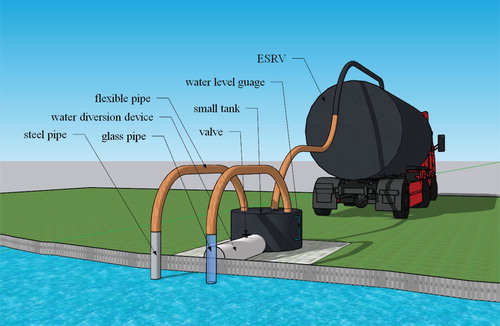
China is a country often plagued by natural disasters (Zhang et al., 2002). Those most frequently occurring include landslides, flooding, and earthquakes. It is not uncommon for individuals to be buried under debris in a natural disaster scenario. China is currently developing a specialized emergency rescue vehicle for excavation and suction, referred to here as the ‘ESRV’, to enhance the efficiency and efficacy of post-disaster rescue missions (Figure 1).

Figure 1. Excavation and suction rescue vehicle.

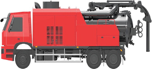
The ESRV is designed to assist rescuers in clearing buried objects swiftly and effectively. The ESRV provides suction via low-vacuum pneumatic conveyance. Tests have shown that the ESRV can gather soil, gravel, and even bricks of a certain diameter into its tank by suction. However, air cannot enter the tank as the vehicle takes in liquid if the suction port is inserted below the liquid level. The liquid in this case hovers in the vertical suction pipe and cannot enter the tank. After landslides or flooding occur, individuals trapped under mud, gravel, or debris underwater must be quickly evacuated. The suction pipe of the ESRV must be carefully, comprehensively designed and tested to ensure it is capable of this task.

A rescue vehicle testing scheme was designed in this study as shown in Figure 2. In this scheme, the suction pipe of the ESRV is not directly applied; rather, a hose is connected to a small storage tank (1 m in height) from which a protruding suction pipe draws liquid into the tank as it is lowered. Tests showed that water did not enter the small tank when placed 1 m above the water because of the relatively weak vacuum therein only – 2 kPa to -8 kPa. However, water easily entered the small tank when the hose protruding from it was connected to a section of the pipe with openings (Figure 2). We found that opening six evenly spaced holes reduced the influence of pipe wall friction upon a rising water flow (though additional holes could be opened as necessary).

Figure 2. Schematic diagram of the liquid suction test.

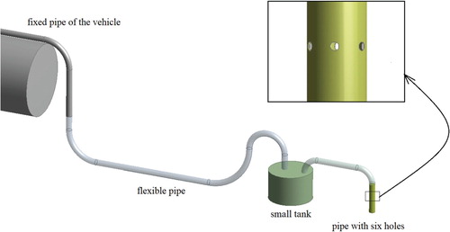
The tests also showed that the position and diameter of the openings affect the suction quality. When openings were placed at the same location, a larger opening diameter created a more intense liquid flow, but more time was required to fill the tank. When openings of the same diameter were placed at different locations, the amount of time required to fill the tank differed accordingly. The liquid suction rate may be improved in accordance with the positions and diameters of the openings and the various parameters of the gas-liquid two-phase flow in the pipe. To this effect, the optimal opening scheme ensures an efficient, effective ESRV.

The flow parameters of the gas-liquid two-phase flow in the pipe can be obtained via the electrical resistance tomography (ERT) monitoring technique (Dickin & Wang, 1996). In addition to measuring flow parameters, ERT can provide images of the flow within the pipe (Lucas et al., 1999). Cho et al. (1999) used ERT to monitor the distribution of air bubbles in the gas-liquid two-phase flow through a vertical pipe. Ma et al. (2001) also used an ERT system to monitor the movement of a gas-liquid two-phase flow in a horizontal pipe.

The flow parameters of the gas-liquid two-phase flow in the pipe can also be obtained by means of calculation. The one-dimensional (1D) two-fluid model created by Taitel and Dukler (1976) has been widely applied for this purpose. Advancements in computer technology have introduced more complex and more accurate computational fluid dynamics (CFD) models as well (de Sampaio et al., 2008). Shoham and Taitel (1984), for example, built a 2D model for predicting stratified turbulent gas-liquid two-phase flow in a slanted pipe. The model can predict the liquid speed field, retention volume, and pressure drop under given flow velocities of gas and liquid as well as physical properties, pipe sizes, and tilt angles. The calculation results are significantly better than the correlation prediction by Lockhart and Martinelli (1949) or the Taitel and Dukler 1D two-fluid model.

Issa (1988) used the standard $k-\epsilon$ turbulence model (proposed by Jones and Launder in 1972) and the Renormalization-group (RNG) turbulence model (proposed by Akai et al. in 1981) to predict stratified gas-liquid two-phase flows in slanted and horizontal pipes. The calculation results were very close to the results obtained by other calculation methods and experimental data. Ghorai and Nigam (2006) used the VOF model (proposed by Hirt and Nichols in 1981) calculate gas-liquid flow in a pipe via the CFD commercial software Fluent 6.0; they compared their calculation and experimental results against the results obtained by Lopez (1994) and Strand (1993) to validate the model. The average error of the prediction of the shear stress distribution and flow profile features was within ± 10%, which confirms the effectiveness of the CFD method. The VOF method and RNG k-ϵ model were also used to study the oil–water flow in three different elbow configurations (Liu et al., 2020). In the case of air-water flow within the dual-fluid atomizer (Minghao et al., 2019), the water absorption improves as the air flow velocity increases. This phenomenon provided a foundation for the work conducted this study.

The ERT monitoring method must be applied to a variety of individual pipe opening schemes to function properly. That is, the experiment must be repeated and the result of each experiment must be analysed separately. Though time-consuming, expensive, and energy-intensive, this method yields highly accurate results. By contrast, the CFD simulation method only requires simulations of pipe models with different opening schemes for analysis. This method saves time and effort, but errors inevitably exist between the calculations and real-world effects. In the present study, we explored the effects of different opening schemes on various parameters in the pipe rather than exact values. Errors within a certain range are thus acceptable and CFD simulation was sufficient for our purposes.

We comprehensively considered the advantages and disadvantages of the ERT technique and the CFD simulation method. We ultimately selected CFD simulation for analyzing the flow parameters of the gas-liquid two-phase in the pipe model with openings. The simulations were conducted in ANSYS 17.0 software. Design Modeler was used to perform 3D modeling of the flow field in the pipe, Mesh was used to complete the model, and Fluent was used for subsequent analyses and calculations. Numerous geometric models were established and the appropriate calculation area was carefully identified before we set parameters and collected results for post-processing.

2. Method

2.1. Pre-processing operation

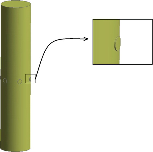
The shape of the movable hose has an uncertain shape, so it was neglected for the purposes of this study. We focused our analysis on a vertical pipe (steel) with openings 1 m in length and 203 mm in section diameter. To identify the effects of different opening positions on the gas-liquid flow in the pipe, we placed one opening along every 5 cm on the pipe amounting to a total of 19 opening positions. We set five different opening diameters for each opening position to observe their respective effects on the gas-liquid flow as well: 5 mm, 10 mm, 15 mm, 20 mm, and 30 mm. This produced a total of 95 different opening schemes. The internal flow field of the pipe with openings was modelled in the Design Modeler tool of ANSYS 17.0, as shown in Figure 3.

Figure 3. 3D model of the flow field in the pipe with openings.

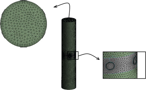
A structured grid is inappropriate for mesh generation in our case as there are many geometric models. We used unstructured grids instead. Unstructured mesh generation is quick and allows for minor changes to the geometric model as necessary. The mesh generation was operated differently for different geometric models based on the same topology structure, which prevented errors caused by re-meshing. One of the grid patterns with the obtained grid partition in Mesh is shown in Figure 4.

Figure 4. Result of mesh generation.

2.2. Setting of fluent boundary conditions

The vertical pipe with openings was connected to the storage tank via a hose, so the negative pressure value at the vertical pipe outlet (upper port) was set to the negative pressure value in the storage tank to simplify the calculation. At the pressure outlet, pressure was set to -5 kPa. (The length of the pipe is 1 m, and the negative pressure in the tank during actual work is between -8 kPa to -2 kPa, with -5 kPa as an intermediate value. If the negative pressure in the tank is -5 kPa, the water level wound reach the middle of the pipe without opening holes. We selected -5 kPa for a convenient analysis of pressure in the tank.)

There were two types of inlets in this model. Six small holes were classified as inlets of the same type. The inlet material in the upper portion of the system was set to air and the inlet material for the lower port to water. The properties of both inlets were set to pressure inlets with pressure intensity of 0. The pipe wall was simulated as a smooth, non-slip wall. The VOF model and standard $k-\epsilon$ model, as discussed in detail below, were utilized for subsequent calculations.

2.3. VOF model

The VOF can be used to model two or more immiscible fluids by solving a single set of momentum equations and tracking the volume fraction of each fluid throughout the domain (ANSYS, 2015). The model is also generally used to calculate time-dependent solutions, so we set a transient state solution instead of a steady state solution for our purposes. The VOF model is primarily composed of the following equations.

1. Volume fraction equation

In the VOF model, different fluid components share a set of momentum equations. The phase volume fraction variable can be used to track the phase interface of each calculation unit.

In each control volume, the sum of the volume fractions of all phases is 1. If volume fraction of the $q$_th phase fluid is ${\alpha }_q$, then (1) $\begin{array}{r}\sum _{q=1}^n{\alpha }_q=1\end{array}$(1) By ignoring the mass transfer between the source term and the different phases, the continuity equation for the $q$ phase can be written as: (2) $\begin{array}{r}\frac{\mathrm{\partial }{\alpha }_q{\rho }_q}{\mathrm{\partial }t}+\mathrm{\nabla }\cdot \left({\alpha }_q{\rho }_q{\overrightarrow{v}}_q\right)=0\end{array}$(2) where ${\rho }_q$ is the density of the $q$ phase fluid and ${\overrightarrow{v}}_q$ is its speed. The interface between phases can be tracked by solving this equation.

(2)	Material property equation

Fluid properties (e.g. density, viscosity) that appear in the transport equation are determined by the sub-phase present in each control body. Taking the density property of two-phase flow as an example, the phases are represented here by subscripts 1 and 2. If the volume fraction of the second phase is tracked (i.e. the volume fraction of the second phase is solved), the density in each unit can be written as: (3) $\begin{array}{r}\rho ={\alpha }_1{\rho }_1+{\alpha }_2{\rho }_2=(1-{\alpha }_2){\rho }_1+{\alpha }_2{\rho }_2\end{array}$(3) Similarly, for the n phase, the average density of the volume ratio of each unit is: (4) $\begin{array}{r}\rho ={\alpha }_1{\rho }_1+{\alpha }_2{\rho }_2+\cdot \cdot \cdot +{\alpha }_n{\rho }_n=\sum _{i=1}^n{\alpha }_i{\rho }_i\end{array}$(4)

(3)	Momentum equation

The density and viscosity in the momentum equation are average volume ratios which can be expressed as follows: (5) $\begin{array}{rl}& \frac{\mathrm{\partial }}{\mathrm{\partial }t}\left(\rho \overrightarrow{v}\right)+\mathrm{\nabla }\cdot \left(\rho \overrightarrow{v}\overrightarrow{v}\right)\\ & =-\mathrm{\nabla }p+\mathrm{\nabla }\cdot \left[\mu \left(\mathrm{\nabla }\overrightarrow{v}+\mathrm{\nabla }{\overrightarrow{v}}^T\right)\right]+\rho \overrightarrow{g}+\overrightarrow{F}\end{array}$(5) where $p$ is the static pressure intensity, $\mu$ is the molecular viscosity, $\mathrm{\nabla }\cdot \left[\mu \left(\mathrm{\nabla }\overrightarrow{v}+\mathrm{\nabla }{\overrightarrow{v}}^T\right)\right]$ is the stress tensor, and $\rho \overrightarrow{g}$ and $\overrightarrow{F}$ are gravity and external force, respectively. The speed field obtained by solving this equation can be shared between phases.

2.4. Standard $k-\epsilon$ turbulence model

The standard $k-\epsilon$ model in ANSYS Fluent falls is a highly practical engineering flow calculation process. Robustness, economy, and reasonable accuracy over a wide range of turbulent flows explain its popularity in industrial flow and heat transfer simulations. It is a semi-empirical model. The derivation of its equations relies on phenomenological considerations and empiricism.

The turbulent kinetic energy $k$ and dissipation rate $\epsilon$ can be obtained by follows: (6) $\begin{array}{r}\frac{\mathrm{\partial }}{\mathrm{\partial }t}\left(pk\right)+\frac{\mathrm{\partial }}{\mathrm{\partial }{x}_i}\left(pk{u}_i\right)=\frac{\mathrm{\partial }}{\mathrm{\partial }{x}_j}\left[\left(\mu +\frac{{\mu }_t}{{\sigma }_k}\right)\frac{\mathrm{\partial }k}{\mathrm{\partial }{x}_j}\right]+G_k-\rho \epsilon \end{array}$(6) (7) $\begin{array}{rl}& \frac{\mathrm{\partial }}{\mathrm{\partial }t}\left(p\epsilon \right)+\frac{\mathrm{\partial }}{\mathrm{\partial }{x}_i}\left(p\epsilon u_i\right)\\ & =\frac{\mathrm{\partial }}{\mathrm{\partial }{x}_j}\left[\left(\mu +\frac{{\mu }_t}{{\sigma }_{\epsilon }}\right)\frac{\mathrm{\partial }\epsilon }{\mathrm{\partial }{x}_j}\right]+C_{\text{1}\epsilon }{G}_k\frac{\epsilon }{k}-C_{2\epsilon }\rho \frac{{\epsilon }^2}{k}\end{array}$(7) where $G_k=-\rho \stackrel{\mathrm{\_}\mathrm{\_}\mathrm{\_}\mathrm{\_}\mathrm{\_}}{{u^{\mathrm{\prime }}}_i{u^{\mathrm{\prime }}}_j}\frac{\mathrm{\partial }{u}_j}{\mathrm{\partial }{x}_i}$ represents the turbulent flow kinetic energy created by the average speed gradient; ${\mu }_t=\rho C_{\mu }\frac{k^2}{\epsilon }$ represents the turbulent viscosity. $C_{\mu }$, $C_{\text{1}\epsilon }$, and $C_{\text{2}\epsilon }$ are constants set to 0.09, 1.44, and 1.92, respectively. ${\sigma }_e$ and ${\sigma }_k$ are the turbulent Prandtl numbers of $k$ and $\epsilon$, ${\sigma }_e\text{ = 1}\text{.0}$ and ${\sigma }_k\text{ = 1}\text{.3}$.

2.5. Mesh independency study

We observed a total of 95 opening schemes in this simulation. We denoted them as $\text{P}(l,d)$, where $l$ represents the distance between the opening position and the liquid inlet (cm) and $d$ is the opening diameter (mm). For example, P(10,20) represents an opening position 10 cm from the liquid inlet with diameter of 20 mm.

Mesh independency study was conducted to exclude the influence of mesh size on the profiles involved in this work. In the meshing stage, five different mesh sizes were set by the relevance option in Mesh software: 0, 20, 40, 60 and 80. A larger relevance value refers to smaller mesh size, more cells.

Different geometric models have a different number of cells after meshing. In our case, the number of the cells was similar in geometric models with the same opening diameter. Therefore, only the P(5,50), P(10,50), P(15,50), P(20,50) and P(30,50) opening schemes were checked for mesh independency. The specific number of cells is shown in Table 1. Most of the profiles referred to here describe the liquid mass flow at liquid inlet of different opening schemes at different time points, so we extracted the profiles of the liquid mass flow rate at the liquid inlet with time.

Table 1. Specific number of cells in different scheme.

Relevance Scheme	0	20	40	60	80
P(5,50)	149265	182848	234688	303789	419746
P10,50)	125062	154455	196035	253927	340270
P(15,50)	113216	141334	177134	226185	296811
P(20,50)	104123	130897	164560	209133	271167
P(30,50)	93614	117861	146263	184978	234975

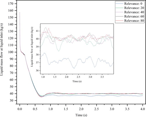
The curves of the P(30,50) scheme are shown in the Figure 5. We found that there is no significant difference in the curves initially, but substantial difference emerged over time. The curve gradually moves upward as the number of cells increases. The gap between curves is small when the relevance value is greater than or equal to 60. Considering that more cells need longer calculation time, we set the value of the relevance value to 60 for our purposes here.

Figure 5. Liquid mass flow at liquid inlet varying over time (P(30,50) scheme).

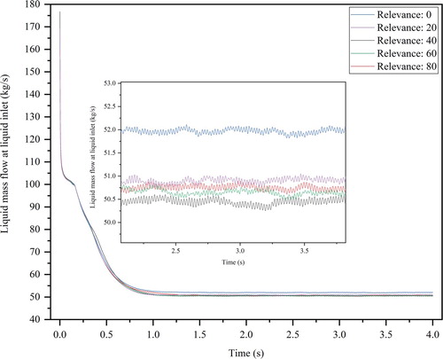
The meshes of the other opening schemes were updated based on the P(30,50) scheme to prevent any errors caused by re-meshing. As shown in Table 1, more cells were generated with a smaller opening diameter and the same relevance value. The curves of the P(20,50) scheme are shown in Figure 6 as the number of cells increases, this curve first moves downward and then upward during the stable fluctuation phase. When the relevance value is greater than or equal to 60, the gap between the curves is very small, in this case indicating no need to further increase the number of cells. The mesh independency profiles of the other schemes are similar to this scheme, so we set the relevance value to 60.

Figure 6. Liquid mass flow at liquid inlet varying over time (P(20,50) scheme).

3. Experimental validation

Simulations are very prone to calculation deviations. We performed tests when the vacuum in the storage tank was stable at -5 kPa on a series of pipes with opening diameters of 15 mm to validate our calculations. We drove the ESRV to secure location where we could ensure that the outside water level would remain constant throughout the absorption experiment. First, we moved the small tank (1 m in height, about 1.5 m in diameter) to a flat plate level with the water surface to prevent the tank from sinking after it was filled. We used two flexible pipes to connect the small tank with a steel pipe and glass pipe each 1.2 m long and 203 mm in diameter, as shown in Figure 7. The two hard pipes were inserted vertically into the water by 20 cm to leave 1 m above the water surface. The opening position of the steel pipe was measured from the water surface rather than the end of the pipe that was under-water.

Figure 7 Schematic of the experiment.

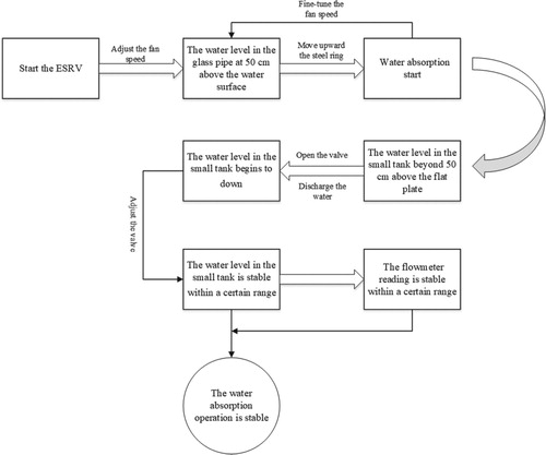
Before starting the water absorption operation, there were lots of preparations to be done. The openings of the steel pipe were blocked with a steel ring before operating the vehicle. The negative pressure of the small tank was generated from a Roots blower of ESRV. The fan speed of the Roots blower was adjusted until the water in the glass pipe rose to 50 cm above the water surface, so that the negative pressure in the small tank was -5 kPa. The steel ring of the steel pipe was moved upward to let air into the pipe, then the water absorption operation began.

During the absorption process, the speed of the fan was fine-tuned to maintain the water level in the glass pipe at 50 cm above the water surface. A diving type electromagnetic flowmeter was installed on the underwater part of the steel pipe to records the volume of liquid flowing into it. A water level gauge was installed on the wall of the small tank to let us know the water level of the tank. When the water level of the small tank beyond 50 cm above the flat plate, the valve on a water diversion device at the bottom would be open to discharge the water. If the water level of the small tank was lower than 50 cm above the flat plat, air would come into the tank from the water diversion device because of the negative pressure inside. As shown in Figure 8, the valve would be adjusted to slow down the water discharge speed until the water level of the tank was stable within a certain range. Once the flowmeter reading was stable within a certain range, which also means the water absorption operation was stable, we recorded all the readings within 10 s and then replaced the steel pipe to conduct the experiment using the next opening scheme.

Figure 8 Flow chart of the experiment.

During the stable absorption stage, the water level in the glass tube still changed (the amplitude was small), which means that the negative pressure value in the small water tank is not a constant. It is difficult for us to stabilize the negative pressure value in the small tank to a constant and it actually changed within a certain range. This would inevitably cause the reading of the flowmeter to fluctuate within a certain range, which would affect the experimental results. So we average the data collected from the flowmeter to reduce the effect.

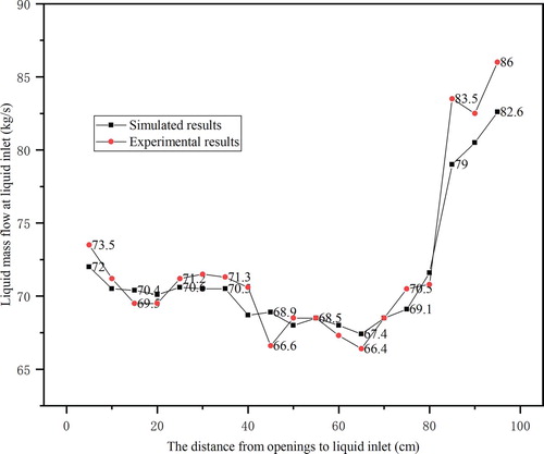
A set of experimental data was collected and compared with the simulation results which were got from the average data at the stable fluctuation stage, as shown in Figure 9. The increasing and decreasing trends of the simulated data are in accordance with the experimental data, which indicates that the simulation results have reference value. We used them to analyse the effects of influence of small openings in the gas-liquid flow in the pipe.

Figure 9. Comparison of experimental and simulated data.

4. Results and analysis

4.1. Analysis of water flow field

Prior to the Fluent operation, we set a monitoring surface at the liquid inlet to record the mass flow under each time step (0.001 s). The recording continued until liquid mass flow at the inlet of the pipe fluctuated within a certain range and exhibited no significant increasing or decreasing trend. We then analysed the effects of the position and diameter of the opening on liquid flow in the pipe.

4.1.1. Opening position effects on liquid flow

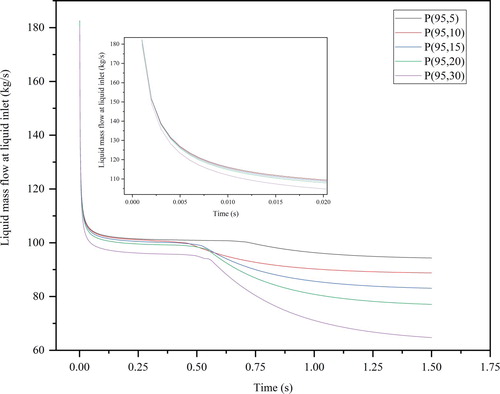
A series of models with opening diameter of 5 mm were simulated as shown in Figure 10. These changes in the mass flow of water at the water inlet with time can be roughly divided into three stages: a rapid decline stage, a slow decline stage, and a stable fluctuation stage.

Figure 10. Liquid mass flow at liquid inlet varying over time (5 mm opening diameter).

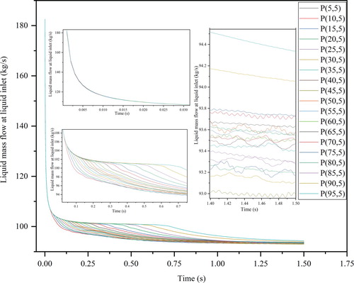
The rapid decline stage occurred immediately after the liquid was sucked into the pipe and lasted for only about 0.02 s. At this point, the curve shows the largest magnitude of decline and a very short duration. The liquid mass flow of then dropped from about 180 kg/s to about 110 kg/s in an instant. This phenomenon may be attributable to the discrete element operation. The curves grew nearly coincident after magnification, suggesting that the opening position of the pipe has little impact on the rapid decline stage.

In the slow decline stage, the curves began to slowly decline and lasted longer. Again, the curves were nearly coincident initially but started to diverge over time. The time point at which each curve diverged, as shown in the figure, does differ – that is, the pipe opening position began to affect the system at this stage. We speculate that the variations in opening position caused liquid to reach the openings at different times; the time points at which the curves diverge are also different in different pipe models. This phenomenon is discussed in greater detail below.

At the stable fluctuation stage, each curve fluctuated steadily and exhibited no significant increasing or decreasing trend with time. The data shown in Figure 10 was only gathered up to the calculation time point of 1.5 s, at which point not all the curves had entered the stable fluctuation stage. Due to the effects of the opening position of the pipe, the time points at which different curves entered this stage differed. They also showed different amplitudes and ranges of fluctuation when they were stable. The opening positions may have affected the airflow disturbance. Our air flow field analysis is also discussed in greater detail below.

The results of our analyses of pipe flow fields in the remaining opening schemes are shown in Figures 11–14. By comparison among the curves, the initial value gaps at the rapid decline stage appear to increase as opening diameter increases. At a certain point, the curves no longer coincided. At the slow decline stage, some curves (e.g. P(5,15), P(10,30)) increased by a certain distance after descending to the lowest point and before entering the stable fluctuation stage.

Figure 11. Liquid mass flow at liquid inlet varying over time (10 mm opening diameter).

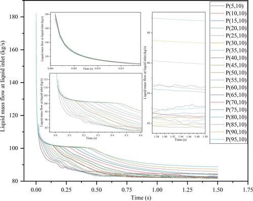
Figure 12. Liquid mass flow at liquid inlet varying over time (15 mm opening diameter).

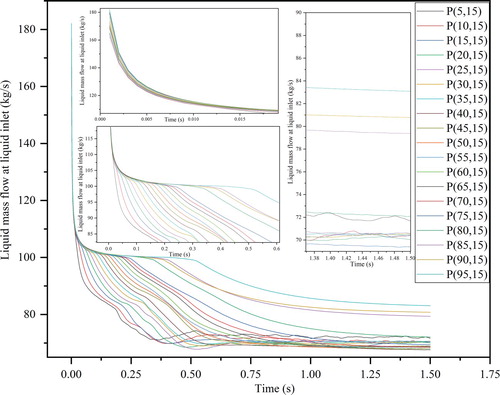
Figure 13. Liquid mass flow at liquid inlet varying over time (20 mm opening diameter).

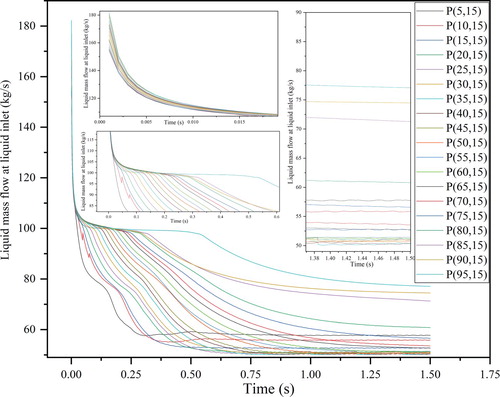
Figure 14. Liquid mass flow at liquid inlet varying over time (30 mm opening diameter).

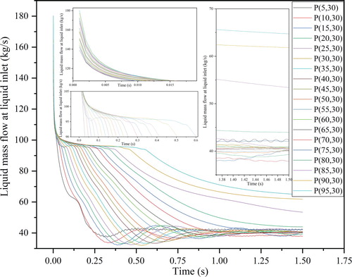
There was no significant difference among the curves for opening schemes with openings far from the water inlet (e.g. P(95,5), P(90,5), P(95,10), P(90,10), P(85,10)) and the other curves at the rapid decreasing stage. However, these curves diverged later and slowly declined at the slow decreasing stage; these curves were significantly different from the others at 1.5 s. In effect, the suction operation efficiency is stronger when pipe opening positions are placed farther away from the liquid inlet.

When the opening position was close to the water inlet, although the time point at which the curve diverged was earlier, the slow decline stage did not last long. In this case, the stable fluctuation state occurred quickly (Figure 13). For these schemes (e.g. P(5,5), P(10,5), P(5,10), P(10,10), P(5,10)), the mass flow of the curves at the stable fluctuation stage was higher than those near the middle of the pipe. That is, the openings near the liquid inlet functioned better than the openings near the middle of the pipe.

4.1.2. Effects of opening diameter on liquid flow in pipe

Based on the analysis presented above, we found that arrangement of opening positions near or far from the liquid inlet is preferable to arrangement near the middle of the pipe. We selected a series of opening schemes with opening positions at 5 cm, 50 cm, and 95 cm from the liquid inlet to assess the effects of the opening diameter on liquid flow in the pipe. The resulting curves of liquid mass flow in the pipe varying over time are shown in Figures 15–17.

Figure 15. Curves of liquid mass flow at liquid inlet varying over time (openings are 5 cm from inlet).

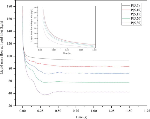
Figure 16. Curves of liquid mass flow at liquid inlet varying over time (openings are 50 cm from inlet).

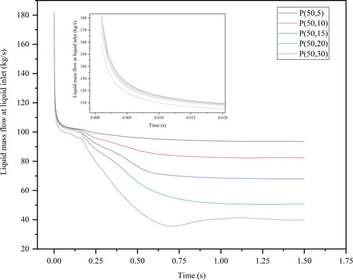
Figure 17. Curves of liquid mass flow at liquid inlet varying over time (openings are 95 cm from inlet).

The curves shown in Figures 15–17 decline in a divergent pattern reflecting certain periods of time. The curve in Figure 15 diverges the earliest, followed by the curve shown in Figure 16, and finally the curve shown in Figure 17. We speculate that this phenomenon is attributable to the liquid flow contacting the air flow at the air intake hole immediately after approaching the positions of the small openings. The opening positions shown in each figure are fixed and the mass flows do not differ as the liquid enters the pipe, so multiple curves thus show disparate states of decline after a fixed period of time. Figure 16 shows the curve most representative of this phenomenon, so we magnified its divergent part to identify the time point at which each curve turned.

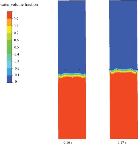
As shown in Figure 18, the time points at which all curves diverge range from about 0.13. s to 0.17 s. We plotted volume fraction cloud diagrams of the liquid phase in the vertical section of the pipe in the P(50,30) opening scheme at 0.13 s, 0.14 s, 0.15 s, and 0.16 s accordingly, as shown in Figure 19. Similarly, the P(50,20) opening scheme at 0.14 s, 0.15 s, and 0.16 s, the P(50,15) and P(50,10) opening schemes at 0.15 s and 0.16 s, and the P(50,5) opening scheme at 0.16 s and 0.17 s were plotted, respectively, to obtain the diagrams shown in Figure 20–23. Comparison of the curves in Figure 19–23 verified our inference.

Figure 18. Curves of liquid mass flow at liquid inlet varying over time (openings are 50 cm from inlet).

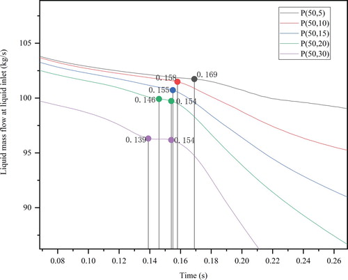
Figure 19. Cloud diagram of liquid volume fraction at vertical pipe section (P(50,30) opening scheme).

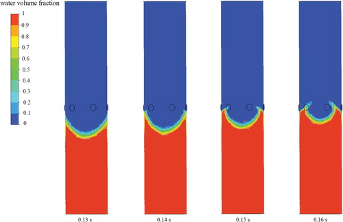
Figure 20. Cloud diagram of liquid volume fraction at vertical pipe section (P(50,20) opening scheme).

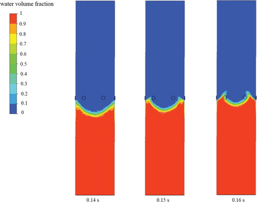
Figure 21. Cloud diagram of liquid volume fraction at vertical pipe section (P(50,15) opening scheme).

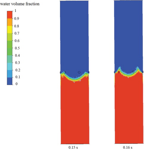
Figure 22. Cloud diagram of liquid volume fraction at vertical pipe section (P(50,10) opening scheme).

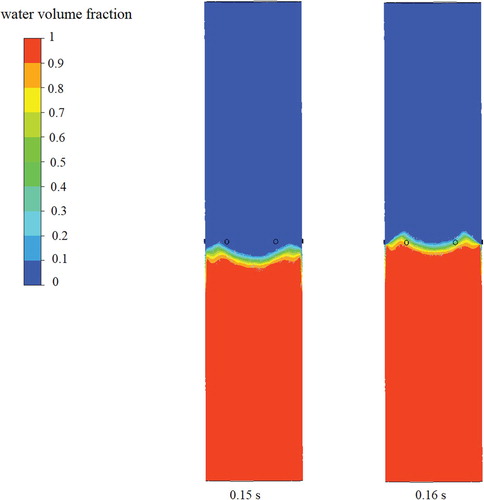
Figure 23. Cloud diagram of liquid volume fraction at vertical pipe section (P(50,5) opening scheme).

The reason for the divergence of the curve is that the water flow contacts with the airflow immediately after it reaches the air inlet. This also explains the phenomenon wherein coincident curves diverge sequentially, as shown in Figures 10–14. We also found that a larger opening diameter results in more pronounced deformation of the liquid surface near the opening. We speculate that this was caused by an increase in air flow caused by the increase in opening diameter. (This speculation was verified as discussed below).

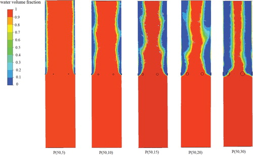
The positions of curves in the stable fluctuation state (Figures 14–17) indicate that once the suction operation reaches the steady state, the liquid mass flow in the pipe has a negative correlation with opening diameter. When the opening position is fixed, a larger opening diameter causes a lower mass flow of liquid in the corresponding pipe. In addition, at the stable fluctuation stage, a larger opening diameter leads to a smaller volume fraction of liquid in the pipe in the gas-liquid two-phase flow above the opening position, as shown in Figure 24.

Figure 24. Cloud diagram of liquid volume fraction at vertical pipe section in steady fluctuation state (P(50,5)-P(50,30) opening schemes).

We also observed a brief rise in the curve shown in Figure 15 during the slow decline stage. This phenomenon emerged in the mass flow curve of the P(5,10) scheme, and grew increasingly obvious with further increase in opening diameter. We observed this phenomenon again in the mass flow curves of the P(50,30) scheme (Figure 16) and in some other (Figures 11–14) where the opening position was located near the water inlet.

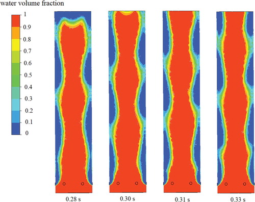
To further explore this phenomenon, we isolated P(5,15), P(5,20), and P(5,30) schemes and drew the curve of the liquid mass flow in their pipes varying over time from 0 to 0.5, as shown in Figure 25. According to the time nodes shown in the figure, we plotted a volume fraction cloud diagram of the liquid phase in the vertical section of the pipe in the P(5,20) opening scheme at 0.24 s-0.32 s (Figure 26). Similarly, we plotted the P(5,30) scheme from 0.27 s-0.32 s and the P(5,15) scheme from 0.28 s-0.33 s (Figures 27 and 28). Figures 26–28 altogether indicate that the transient rise of these curves occurred immediately after the liquid flow reached the pipe outlet.

Figure 25. Curves of liquid mass flow at liquid inlet varying over time (openings are 5 cm from inlet).

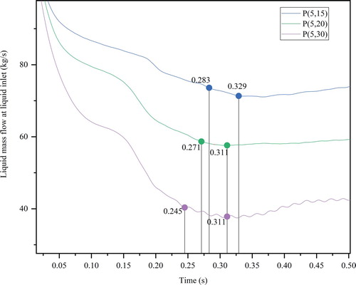
Figure 26. Cloud diagram of liquid volume fraction at vertical pipe section (P(50,30) opening scheme).

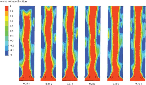
Figure 27. Cloud diagram of liquid volume fraction at vertical pipe section (P(50,20) opening scheme).

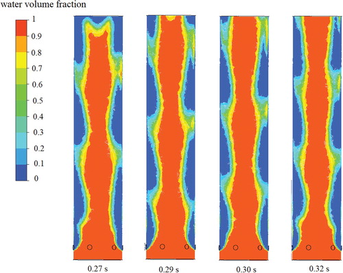
Figure 28. Cloud diagram of liquid volume fraction at vertical pipe section (P(50,15) opening scheme).

We speculate that due to the low opening position in the above cases, the liquid in the pipe was continually lifted by flowing air after the liquid entered the pipe. As the suspended liquid column grew increasingly lengthy, the mass flow of liquid at the inlet rapidly decreased. As liquid flowed out from the outlet, the gas-liquid two-phase flow state in the pipe changed slightly. During this change, the liquid mass flow at the water inlet briefly increased. The mass flow of the liquid at the liquid inlet entered a stable fluctuation state immediately after this change process ended.

4.2. Air flow field analysis

We next analysed the effects of the positions and diameters of openings on the air flow field in the pipe.

4.2.1. Opening positions affect air flow field in pipe

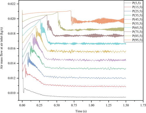
As the curve of air flow in the pipe varying over time fluctuated greatly, it was difficult to observe when all calculation results were plotted into a single line chart. In observing the effects of positions of openings with a uniform diameter of 5 mm on the pipe’s air flow, we isolated data obtained from the P(5,5), P(5,15), P(5,25) … P(5,85), and P(5,95) opening schemes for the sake of convenience. As shown in Figure 29, the changes in the mass flow rate of the air at the air inlet varying with time can be roughly divided into four stages: a rapid decline stage, a steady rise stage, a fluctuation decline stage, and a stable fluctuation stage.

Figure 29. Curves of air mass flow at air inlet varying over time (openings are 5 cm from inlet).

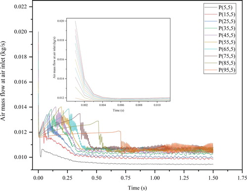
The rapid decline stage was short and the decline magnitude was large. The original curve was almost vertical. After magnifying the original curve, we found that despite the brevity of this period of time, the initial values of various curves differed due to the differences in the opening positions. The resulting curves also differed by scheme.

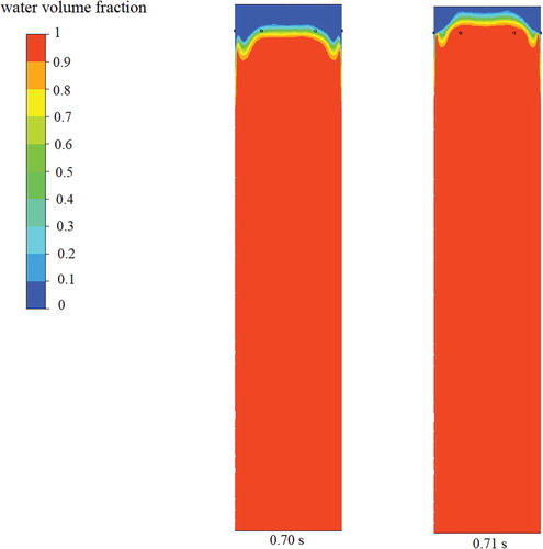
During the steady rise stage, each curve started to rise steadily without fluctuations. However, the rise time and effect of each curve was different. An opening position closer to the water inlet would lead to a shorter the rise time of the air mass flow rate. To explain this phenomenon, through the time nodes in Figure 30, we plotted the volume fraction cloud diagrams of the vertical cross-section liquid phase in the pipe of the P(75,5) opening scheme at 0.35 s and 0.36 s, as shown in Figure 31. Similarly, we plotted diagrams for the P(85,5) scheme at 0.51 s and 0.52 s, and for the P(95,5) scheme at 0.70 s and 0.71 s, respectively, as shown in Figures 32 and 33.

Figure 30. Curves of air mass flow at air inlet varying over time (openings are 5 cm from inlet).

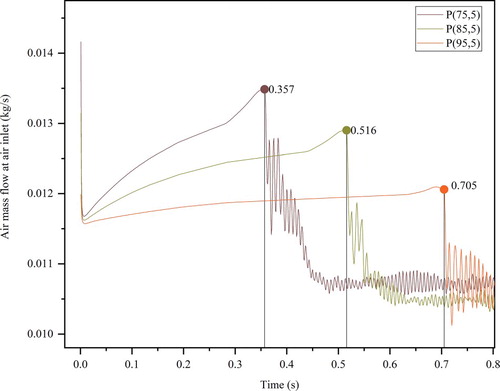
Figure 31. Cloud diagram of liquid volume fraction at vertical pipe section (P(75,5) opening scheme).

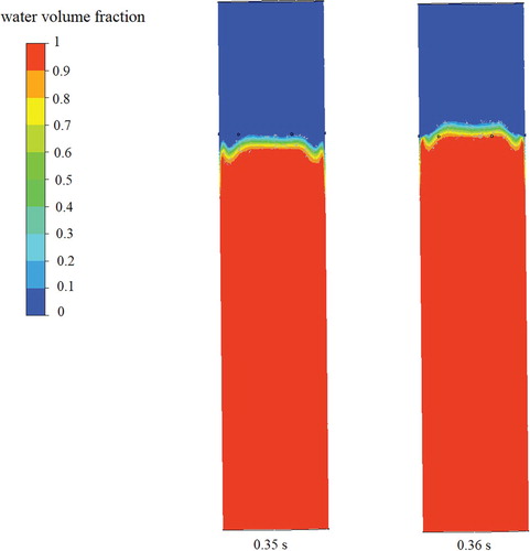
Figure 32. Cloud diagram of liquid volume fraction at vertical pipe section (P(85,5) opening scheme).

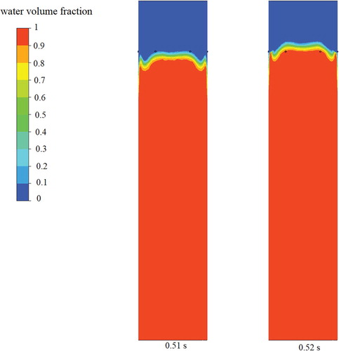
Figure 33. Cloud diagram of liquid volume fraction at vertical pipe section (P(95,5) opening scheme).

As shown in Figures 31–33, the time points corresponding to the turning point fell just within the time period when the water flow reached the air inlet. In other words, the slow rise stage of the air mass flow rate occurred before the liquid flow reached the air inlet. Due to the differences in opening positions, the time it took for the liquid flow to reach the air inlet also differed among various schemes. An opening position closer to the water inlet created a shorter air mass flow slow rise stage.

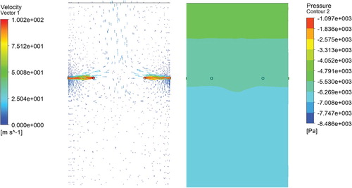
We drew a vector diagram of the air speed in the pipe around the P(85,5) scheme openings in the steady rise stage (that is, when the liquid flow had not reached the opening position), as shown in Figure 34. After the air flow entered via the small opening, a portion of it moved upwards to the outlet while the remaining air flowed toward the liquid, then returned back to the vicinity of the pipe wall. Figure 34 also shows where the shape of the liquid surface was created by the trajectory of the air flow. We speculate that when the flowing air reached the liquid level from the small openings and then returned back from the pipe wall, a portion of it was swept into the upward air flowing at the openings. When the air flow returned to the liquid surface again, the air was thinner; this caused the static pressure at the liquid surface to decrease, thus pushing the liquid upward. The static pressure distribution in the pipe, as shown in Figure 35, supports this speculation.

Figure 34. Comparison of vertical section speed vector of pipe and volume fraction of liquid during steady rise stage (scheme P(85,5), 0.49 s).

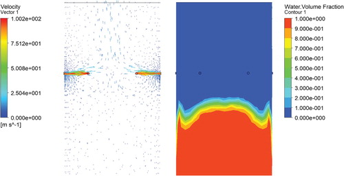
Figure 35. Comparison of vertical section speed vector of pipe and static pressure distribution during steady rise stage (scheme P(85,5), 0.49 s).

Each curve fluctuated to varying extent in the fluctuation decline stage, forming a trend that was passed on to the next stage. At the stable fluctuation stage, the degree of fluctuation in each curve differed but all fell within a certain range and showed no significant rise or decline. The curve shown in Figure 36 was obtained by offsetting the curve shown in Figure 29. As shown in Figure 36, the maximum amplitude of the curve fluctuation increased as the distance from the opening position to the liquid inlet increased, but the frequency of the occurrence of the maximum amplitude decreased. This phenomenon may be attributable to the fact that openings at different positions exerted different effects on the air flow disturbances discussed above. The cause of this phenomenon was not identified.

Figure 36. Curves of air mass flow at air inlet varying over time (after offset).

4.2.2. Opening diameter affects air flow field in pipe

Pipes with opening positions 5 cm, 50 cm, and 90 cm from the water inlet were selected to monitor the air flow inward. The results are shown in Figures 37–39.

Figure 37. Curves of air mass flow at air inlet varying over time (openings are 5 cm from liquid inlet).

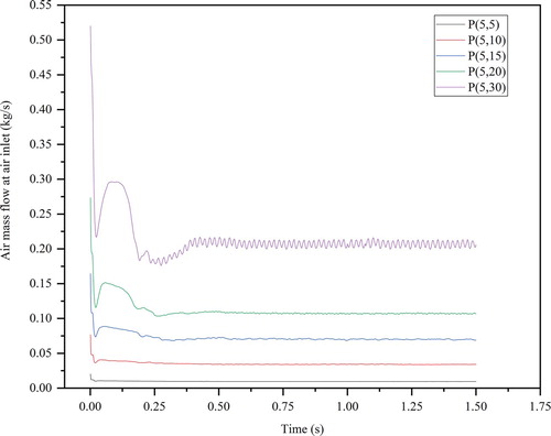
Figure 38. Curves of air mass flow at air inlet varying over time (openings are 50 cm from liquid inlet).

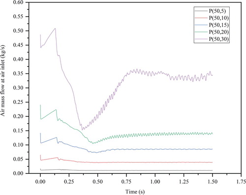
Figure 39. Curves of air mass flow at air inlet varying over time (openings are 95 cm from liquid inlet).

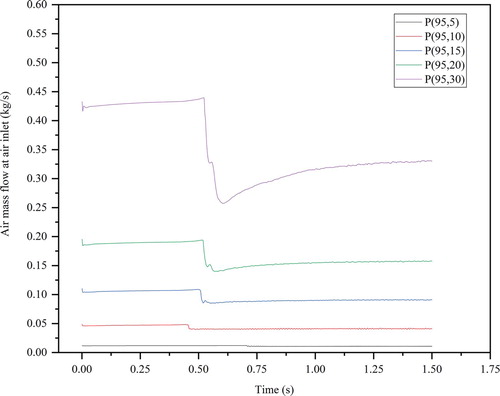
Based on a comparison of the data shown in Figure 37–39, we conclude that when the degree of vacuum in the tank is -5 kPa, the mass flow of air at the air inlet is positively correlated with opening diameter. A larger opening diameter appeared to cause greater air mass flow at the inlet.

Opening diameter also plays an important role in all four stages of the air mass flow curve. At the rapid decline stage, the opening diameter determines the initial value and the degree of decline in the curve. A larger opening diameter leads to a higher initial value in the curve and a greater degree of its decline. At the steady rise stage, a larger opening diameter leads to a higher rise in the curve. In the steady decline stage, a larger opening diameter led to a higher degree of decline in the curve. At the end of this stage, when the opening diameter was greater than 10 mm, there was an increase in fluctuations as well. At the steady fluctuation stage, opening diameter again determined the fluctuation amplitude of the curve. As shown in Figure 38, a larger opening diameter caused a higher curve fluctuation amplitude.

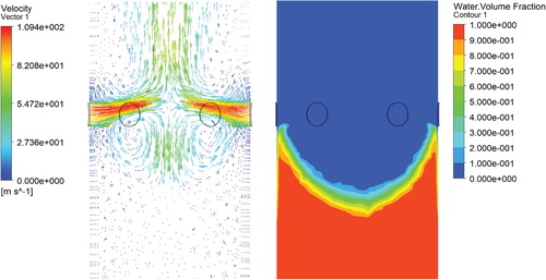
To determine why a larger opening diameter creates more significant deformation of the liquid surface in the vicinity of the opening, we isolated P(50,15), P(50,20), and P(50,30) schemes for further analysis. First, the time points to be analysed were obtained from Figures 19–21 as 0.15 s, 0.15 s, and 0.14 s for P(50,15), P(50,20), and P(50,30), respectively. A comparison between the speed vector near the pipe opening corresponding to the time point and liquid volume fraction in the pipe’s vertical section is provided in Figures 40–42. It appears that the air flow into the pipe increased as the opening diameter increased, thus creating an increase in the vortex formed near the air inlet and in the deformation of the liquid surface.

Figure 40. Comparison of vertical section speed vector of pipe and volume fraction of liquid (scheme P(50,15), 0.15 s).

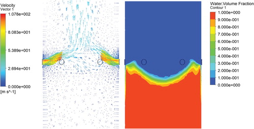
Figure 41. Comparison of vertical section speed vector of pipe and volume fraction of liquid (scheme P(50,20), 0.15 s).

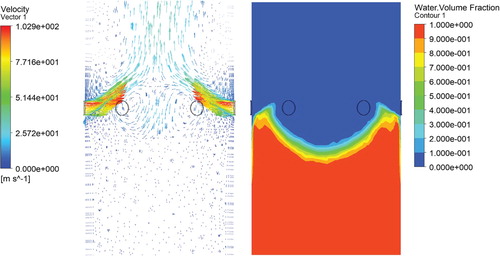
Figure 42. Comparison of vertical section speed vector of pipe and volume fraction of liquid (scheme P(50,30), 0.14 s).

4.3. Effects of pipe openings on liquid suction speed

Rules for the curves of the mass flow of air and liquid varying over time, as described above, were obtained on a small time scale. To make reasonable suggestions for openings of the ESRV during actual operation, it is necessary to compare the liquid suction speeds corresponding to additional schemes.

We next compared the mass flow of liquid at the pipe’s liquid inlet in a typical ESRV in a stable state corresponding to different opening schemes. Calculation results for each example in the stable fluctuation stage were taken and averaged to obtain the results listed in Table 2 and displayed in Figure 43.

Figure 43. Mass flow at liquid inlet corresponding to various opening schemes.

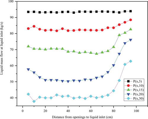
Our conclusions based on Figure 43 can be summarized as follows.

1. A larger opening diameter leads to smaller mass flow at the liquid inlet.

2. When the opening diameter is 5 mm, the mass flow at the liquid inlet is less affected by changes in opening position; when the opening diameter is greater than or equal to 10 mm, liquid mass flow at the inlet increases gradually as the opening position changes.

3. When the diameter of the opening is greater than or equal to 10 mm, the liquid mass flow at the liquid inlet decreases first, then increases as the distance from the opening to the liquid inlet increases.

4. The effects of openings placed at the upper end of the pipe are significantly better than those of openings at the bottom portion of the pipe

Table 2. Inlet mass flow (kg/s) data corresponding to various pipe opening schemes.

D/mm L/cm	5	10	15	20	30
5	93.45	83.1	72.0	57.8	42.3
10	93.5	84.5	70.5	55.8	37.8
15	93.2	82.7	70.4	52.8	40.4
20	93.2	82.0	70.1	51.1	40.0
25	93.3	82.2	70.6	51.1	40.0
30	93.1	81.7	70.5	51.0	41.8
35	93.4	83.0	70.5	50.5	40.9
40	93.5	81.8	68.7	50.3	41.2
45	93.0	81.9	68.9	50.8	39.8
50	93.6	82.3	68.0	50.6	40.3
55	93.6	82.2	68.5	51.4	39.6
60	93.5	82.1	68.0	51.3	41.0
65	93.6	82.0	67.4	52.5	40.1
70	93.7	82.2	68.25	53.3	40.7
75	93.6	83.6	69.1	56.0	41.7
80	93.4	83.6	71.6	60.3	44.4
85	93.1	85.5	79.0	67.4	50.8
90	93.8	87.0	80.45	74.0	60.8
95	93.9	88.5	82.6	76.1	62.8

Legend: L is the distance from the opening position to the water inlet, D is the opening diameter.

5. Conclusion

In this study, we performed CFD simulations of various suction pipe opening schemes in an ESRV. We analysed the effects of various positions and diameters of openings on the gas-liquid two-phase flow in the pipe over a small time scale. We then compared the suction efficiency corresponding to different opening schemes. Our conclusions can be summarized as follows.

1. Opening diameter significantly affects liquid mass flow while opening position does not.

In the calculation example given in this paper, the effects of the opening diameter on the gas-liquid two-phase flow in the pipe are greater than those of the opening position. Curves of liquid mass flow at the liquid inlet were compared with those of the air mass flow at the air inlet varying with time. We found that the effects of the opening diameter emerge immediately upon liquid entering the pipe. Our assertion that opening diameter has a greater impact on the liquid mass flow than opening position were confirmed by comparing the interval between various curves during stable fluctuation.

(2)	Different opening positions and opening diameters exert different effects on the gas-liquid two-phase flow in the pipe.

The effects of the opening position on the gas-liquid two-phase flow in the pipe are only significant when the pipe opening diameter reaches a certain size. The mass flow of liquid in the pipe is also lower when openings are placed in the middle of the pipe than when they are placed at both ends. As the opening position moves farther from the liquid inlet, the mass flow of the liquid entering the pipe decreases first and then increases. A larger pipe opening diameter results in lower liquid mass flow into the pipe. The pipe opening diameter not only determines the shape of the liquid surface before it reaches the opening position, but also determines the volume fraction of the liquid phase in the gas-liquid two-phase flow above the opening position.

(3)	Liquid suction performance is optimal when small-diameter openings are placed in the upper part of the pipe.

We also compared the values corresponding to these curves in a stable fluctuation state. Generally, the liquid suction performance is optimal when small-diameter openings are placed in the upper part of the pipe.

The results presented here may provide a workable reference for ESRV optimization at rescue sites in cases of debris overflow and flooding. However, our conclusions are only applicable to the absorption of water in vertical opening pipes. Further research is needed to investigate cases where the suction pipe has a certain inclination angle, or when the material to be absorbed is mud or muddy water.

Disclosure statement

No potential conflict of interest was reported by the author(s).

Additional information

Funding

This work was supported by Ministry of Science and Technology of the People's Republic of China (National Key Research and Development Program of China: 2016YFC0802900).