Dynamic analysis of an elastic ring squeeze film damper supported rotor using a semi-analytic method

Abstract

To speed up the calculation of dynamic analysis for elastic ring squeeze film dampers (ERSFDs) and investigate the dynamic characteristics of ERSFD-rotor systems, a semi-analytic method (SAM) is proposed for analyzing oil film pressure and force. This method is subsequently verified by comparison with numerical simulation and experimental results. Based on this SAM, an improved dynamic model of an ERSFD-supported rotor is developed by coupling the kinetic equations of the rotor with the determination of elastic deformation. Using this method, the oil coefficients and vibration behaviors of the rotor such as the amplitude–frequency relation and the influence of sudden excitation are investigated. The results reveal that the equivalent oil coefficients and damping ratio of the system can be increased significantly by the adoption of ERSFDs. Therefore, the nonlinear bi-stable response occasionally occurring in traditional squeeze film damper (SFD) supported rotors is effectively suppressed and the transient vibration process caused by sudden unbalanced excitation action is significantly shortened. The SAM enables one to reduce the computation time of the previous method by more than 90%. Such a reduction greatly improves the computational efficiency.

KEYWORDS:

• Elastic ring squeeze film damper
• semi-analytic method
• dynamic characteristics
• rotor dynamics

1. Introduction

Using squeeze film dampers (SFDs) in controlling the vibration of rotor systems has been common in aero engines. Compared with traditional SFDs, the merits of elastic ring squeeze film dampers (ERSFDs) are their small size and light weight (Chen et al., 2016; Han et al., 2019; Han & Ding, 2018; Lei, 2006; Siew et al., 2002; Wang et al., 2017; Wang et al., 2018; Wang et al., 2019; Zhang & Ding, 2015). In addition, ERSFDs have an enhanced ability to suppress oil film nonlinearity. Thus, ERSFDs have potential applications in centrifuges and turbines.

As shown in Figures 1 and 2(a), cited from Han et al. (2019), an elastic ring with internal and external bosses is embedded to divide the oil film of the SFD into two layers. The embedded elastic ring provides extra support to the rotor and suppresses nonlinear levels of oil pressure. Based on the geometrical characteristics of equally separated oil chambers, Zhou Min et al. (1998) developed Reynolds equations for two layers of oil films by using fluid lubrication theory. The oil pressures were obtained using the finite difference method (FDM), in which the influence of the bosses on the oil chamber segmentation is considered. The dynamic analysis of oil force for ERSFDs is a typical fluid–solid interaction problem. By dividing the elastic ring into several ring segments and assuming each ring segment to be a simple support plate, Dai and Wang (1994) analyzed the effect of ring deformation on oil pressure, the accuracy of which still needs to be improved. In Jie et al. (2006) and Zhang and Ding (2015), the oil coefficients could be investigated by coupling the deformation analysis in the commercial software ANSYS^® with fluid lubrication theory, although using this method it is not easy to analyse the effect of ERSFD on rotor response. Based on Kirchhoff theory, Han et al. (2019) developed a coupling method for simulating the ring–oil interaction in ERSFDs and analyzing the response of the rotor. But the calculation of oil pressure for ERSFDs is still time-consuming using the above method, so developing a more efficient simulation procedure for the dynamic analysis of ERSFDs is necessary.

Figure 1. Illustration of the rotor supporter on an ERSFD and a mouse cage.

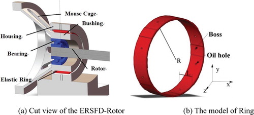
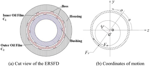
Figure 2. Schematic illustration of an ERSFD.

Recently, some novel kinds of SFDs similar to the ERSFDs have been proposed and investigated by analytical or semi-analytical methods. Holmes (1972) proposed theoretical expressions for the oil film pressure of SFDs without misalignment based the assumptions of open end boundaries and short bearings. Karimulla et al. (2019) investigated the oil force of an SFD experimentally and analytically under circular-centered orbit (CCO) motion. Zhang et al. (1993) developed a nonlinear theoretical expression for oil force by simplifying the Navier–Stokes equations based on the short bearing assumption. Chen et al. (2014) and Zhu et al. (2002) analyzed the dynamic response of an SFD-rotor system based on the short bearing assumption. Based on the 2π-film and π-film assumption, San Andres and Vance (1988) proposed an analytical oil force formula for the SFD to investigate the dynamic response of the rotor, which indicated that the probability of a bi-stable response decreased moderately with increasing fluid inertia. The instability phenomenon caused by self-excited vibrations in a fully-floating ring-bearing-rotor system was investigated by Schweizer (Boyaci et al., 2015). Based on the assumption of short bearings, Zhou et al. (2014) analyzed the dynamic characteristics of a floating ring SFD-bearing-rotor system. Changsheng and Xixuan (1995)proposed hydrostatic squeeze film dampers (HSFDs) to reduce the nonlinear level of oil pressure in SFDs and developed an analytical oil pressure expression for HSFDs. Abed et al. (2017) analysed the dynamic characteristics of a three-pad HSFD based on the π-film assumption using an analytical method. Guan et al. (2019) investigated the influence of operating conditions such as speed on a centrifugal compressor supported by magnetic bearings, using theoretical and experimental methods. The computational fluid dynamics (CFD) technique was adopted to solve fluid–solid interaction problems in recent investigations (Akbarian et al., 2018; Ghalandari et al., 2019; Salih et al., 2019). Hou et al. (2017, 2019) analyzed the bifurcation and primary resonance of a dual-rotor system using a semi-analytical procedure.

To the authors’ knowledge, there is still no semi-analytic method for analyzing the dynamic characteristics of ERSFD rotors up to now. In order to improve the computational efficiency of ERSFD-rotor dynamics, a semi-analytical method (SAM) is proposed in this paper, as presented in Section 2. Based on this method, the dynamic characteristics of an ERSFD are discussed and the results are verified by comparison with numerical calculations in Section 3. In Section 4, the dynamic responses of an ERSFD rotor are investigated by SAM, numerical, and experimental methods, respectively. Finally, conclusions are summarized.

2. The semi-analytical method

2.1. Reynolds equations

Rigid boundaries are assumed at the outer surface of the bushing and inner surface of the housing surface in the ERSFD, the transient Reynolds equations are given by (Han et al., 2019) (1) $\begin{array}{rl}& \frac{1}{R^2}\frac{\mathrm{\partial }}{\mathrm{\partial }\theta }{h}_1^3\frac{\mathrm{\partial }{p}_1}{\mathrm{\partial }\theta }+\frac{\mathrm{\partial }}{\mathrm{\partial }x}\left(h_1^3\frac{\mathrm{\partial }{p}_1}{\mathrm{\partial }x}\right)=-12\mu \mathrm{\Omega }\left(\frac{\mathrm{\partial }{h}_1}{\mathrm{\partial }\theta }-\frac{\mathrm{\partial }r}{\mathrm{\partial }\theta }\right)\\ & +12\mu \frac{\mathrm{\partial }{h}_1}{\mathrm{\partial }t}+\rho h_1^2\frac{{\mathrm{\partial }}^2{h}_1}{\mathrm{\partial }{t}^2}\end{array}$(1) and (2) $\frac{1}{R^2}\frac{\mathrm{\partial }}{\mathrm{\partial }\theta }{h}_2^3\frac{\mathrm{\partial }{p}_2}{\mathrm{\partial }\theta }+\frac{\mathrm{\partial }}{\mathrm{\partial }x}\left(h_2^3\frac{\mathrm{\partial }{p}_2}{\mathrm{\partial }x}\right)=12\mu \frac{\mathrm{\partial }r}{\mathrm{\partial }t},$(2) where p₁ and p₂ are the inner and outer oil pressures, respectively. Moreover, R represents the radius, μ is the viscosity of the oil, and Ω is the precessional velocity of the journal. The axial and circumferential coordinates are x and θ, respectively, as shown in Figure 2(b). For the structure shown in Figure 2(a), note that c₁ and c₂ are the original clearances of the oil chambers, thus h₁ and h₂, the oil film thicknesses resulting from the journal precession and deformation of the elastic ring, are calculated as (3) $\left\{\begin{array}{c}{h}_1=c_1+r\left(\theta \right)+e\cos \theta \\ \frac{\mathrm{\partial }{h}_1}{\mathrm{\partial }\theta }=\frac{\mathrm{\partial }r}{\mathrm{\partial }\theta }-e\sin \theta \\ \frac{\mathrm{\partial }{h}_1}{\mathrm{\partial }t}=\dot{r}+\dot{e}\cos \theta \end{array}\right.\text{and}\left\{\begin{array}{c}{h}_2=c_2-r\left(\theta \right)\\ \frac{\mathrm{\partial }{h}_2}{\mathrm{\partial }\theta }=-\frac{\mathrm{\partial }r}{\mathrm{\partial }\theta }\\ \frac{\mathrm{\partial }{h}_2}{\mathrm{\partial }t}=-\dot{r}\end{array}\right.$(3) with e, r standing for the precessional eccentricity of the bushing and the ring deformation, and $\dot{e}$, $\dot{r}$ are their first derivatives. ε = e/c₁ stands for the eccentricity ratio.

It is very difficult to solve Equations (1) and (2) analytically, so the FDM is usually applied to solve them and thus to obtain the oil pressures. But FDM processing is often quite time consuming, and it is not suitable for the complicated dynamic analysis of the ERSFD-rotor system.

2.2. Semi-analytical expressions for oil pressure

In practice, because the axial length of the damper is usually less than 1/4 of its diameter (Bangchun et al., 2000; Zhu et al., 2002), the variation of oil film pressure along the axial direction is more obvious than that along the circumferential direction during operation. The following assumptions are adopted.

1. The oil film thickness is very thin, hence the velocity gradient along the direction of thickness is much smaller than that in other directions.

2. The fluid is an incompressible Newtonian fluid.

3. The temperature effect of the fluid is neglected.

4. The damper is not tilted in the axial direction.

5. The short bearing assumption is adopted.

6. The outer boss of the elastic ring is in tight contact with the housing and the inner boss is in tight contact with the bushing of the mouse cage. The elastic ring is non-floating.

7. Because the Reynolds number of this damper is quite small, the inertia term of the inner oil film is neglected.

Thus, ignoring the first terms and inertia term in Equations (1) and (2) results in the following equations: (4) $\frac{\mathrm{\partial }}{\mathrm{\partial }x}\left({h_1}^3\frac{\mathrm{\partial }{p}_1}{\mathrm{\partial }x}\right)=-12\mu \mathrm{\Omega }\left(\frac{\mathrm{\partial }{h}_1}{\mathrm{\partial }\theta }-\frac{\mathrm{\partial }r}{\mathrm{\partial }\theta }\right)+12\mu \frac{\mathrm{\partial }{h}_1}{\mathrm{\partial }t}$(4) and (5) $\frac{\mathrm{\partial }}{\mathrm{\partial }x}\left({h_2}^3\frac{\mathrm{\partial }{p}_2}{\mathrm{\partial }x}\right)=12\mu \frac{\mathrm{\partial }r}{\mathrm{\partial }t}.$(5)

The boundary conditions at both axial ends of the damper are as follows: (6) $p\left(\theta ,\frac{L}{2}\right)=p_{e1},p\left(\theta ,-\frac{L}{2}\right)=p_{e2},x=-\frac{L}{2}\text{or}\frac{L}{2},$(6) where p_e1 and p_e2 are the initial pressures at the axial ends of the damper, respectively, which are zero while there are no seals in the damper, as shown in Equation (9). Integrating Equations (4) and (5), we obtain the inner oil pressure expression and outer oil pressure expression as (7) $\begin{array}{rl}{p}_1\left(\theta ,z\right)& =\frac{6\mu }{{(c_1+r(\theta )+e\cos \theta )}^3}\left(\mathrm{\Omega }e+\frac{\mathrm{\partial }r}{\mathrm{\partial }t}+\dot{e}\cos \theta \right)\\ & \cdot \left(z^2-\frac{L^2}{4}\right)+Q_{1}x+Q_2\theta \in {\theta }_i,{\theta }_j\end{array}$(7) (8) $\begin{array}{rl}{p}_2\left(\theta ,z\right)& =\frac{6\mu }{{(c_2+r(\theta \left)\right)}^3}\cdot \left(-\frac{\mathrm{\partial }r}{\mathrm{\partial }t}\right)\cdot \left(z^2-\frac{L^2}{4}\right)+Q_{1}x\\ & +Q_2\theta \in {\theta }_i,{\theta }_j,\end{array}$(8) (9) $p_1\left(\theta ,z\right)=0;p_2\left(\theta ,z\right)=0;\theta \in {\theta }_{bi},{\theta }_{bj};i=1,2,\dots ,8,$(9) where $Q_1=\frac{p_{e1}-p_{e2}}{L},Q_2=\frac{p_{e1}+p_{e2}}{2},$where θ_bi and θ_bj are the lower and upper circumferential angles of the position of the boss, respectively. To consider the influence of the cavitation, the π-film assumption is adopted in calculating the oil pressure.

2.3. Bearing capacity

Integrating the oil film pressure from the lower boundary angle θ_i to the upper boundary angle θ_j of one oil film chamber using Simpson integration, the radial and circumferential oil forces are calculated by (10) $\left[\begin{array}{c}{F}_r\\ F_{\theta }\end{array}\right]=-{\int }_{{\theta }_1}^{{\theta }_2}\left({\int }_{-\left(L/2\right)}^{L/2}{P}_1\text{d}x\right)\left[\begin{array}{c}-\cos \theta \\ \sin \theta \end{array}\right]R\text{d}\theta ,$(10) the nonlinear oil forces in the y- and x-directions are derived from Equation (11): (11) $\left[\begin{array}{c}{F}_z\\ F_y\end{array}\right]=\begin{array}{c}{F}_r\cdot \cos \varphi -F_{\theta }\cdot \sin \varphi \\ F_r\cdot \sin \varphi +F_{\theta }\cdot \cos \varphi ,\end{array}$(11) where ϕ represents offset angle between the z-axis and the radial direction of the journal.

2.4. Motion equations

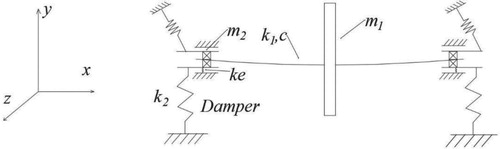
The dynamic equations of a symmetrical ERSFD supported Jeffcott rotor, depicted in Figure 3, are deduced to be (12) $\left\{\begin{array}{c}{m}_1{\ddot{z}}_1+2k_1{z}_1-z_2+c{\dot{z}}_1=m_1{\omega }^2{e}_u\cos \left(\omega t\right)\\ m_1{\ddot{y}}_1+2k_1{y}_1-y_2+c{\dot{y}}_1=m_1{\omega }^2{e}_u\sin \left(\omega t\right)\\ m_2{\ddot{z}}_2+k_1{z}_2-z_1+\left(k_2+k_e\right)z_2=F_z\\ m_2{\ddot{y}}_2+k_1{y}_2-y_1+\left(k_2+k_e\right)z_2=F_y,\end{array}\right.$(12) where m₁ is the lumped mass at the disk, m₂ is the equivalent mass at one end of the shaft involving the mass of the bearing, damper, and shaft. Here, e_u is the unbalanced distance of the disk. Moreover, 2k₁ is the stiffness of the shaft, k_e is the elastic ring's equivalent stiffness, k₂ is the stiffness of the bearing mouse cage, and c is the equivalent linear damping caused by friction and the effects of aerodynamic factors. z₁, y₁ stand for displacements at the disk, and z₂, y₂ for displacements at the end of the shaft. Equations (12) are solved by the Runge–Kutta method.

Figure 3. Dynamic model of a rotor supported on two ERSFDs.

Defining a dimensionless speed ratio as (13) $\lambda =\frac{\omega }{p_{1n}},$(13) with p_1n referring to the first natural frequency of the disk/shaft system, which can be calculated by Equation (17(17) $\begin{array}{rl}P{n}_1& =\sqrt{\frac{E_1-\sqrt{2E_1^2-16E_2}}{4m_1{m}_2}},\\ P{n}_2& =\sqrt{\frac{E_1+\sqrt{2E_1^2-16E_2}}{4m_1{m}_2}}\end{array}$(17) ).

2.5. Procedure of the semi-analytical method

The solution procedure is illustrated in Figure 4.

1. The processing states of the rotor are used as initial conditions to calculate the inner oil film thickness and the inner oil pressure by using Equations (3) and (7).

2. The deformation of the elastic ring r is calculated according to the inner oil pressure by using the finite element method presented in Han et al. (2019). Then, the thickness of the two layers of oil film after deformation is determined from Equation (3).

3. Oil pressures and oil forces are obtained from Equations (7)–(11).

4. The oil force is adopted to advance the simulation in order to reach the next processional state of the rotor by using Equations (12). This process continues until the end of the steady state. Then the oil coefficients are calculated from Equation (14).

Figure 4. Flow illustrating the semi-analytical method (SAM).

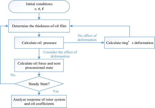
Compared with Han et al. (2019), there is no convergence judgment of the FDM in this procedure, which also helps to improve the speed of calculation (Table 1).

Table 1. Parameters of the ERSFD-rotor system.

Parameter	Value	Parameter	Value
Lubricant viscosity, μ	5 cP	Stiffness of shaft, k1	0.874×10^6 N·m^−1
Mass of disk, m1	6 kg	Elasticity modulus, E	1.96×10^5 MPa
Mass of end of shaft, m2	2 kg	Density of ring	7850 kg·m^−3
Inner diameter of damper	80 mm	Poisson ratio	0.3
Outer diameter of damper	83 mm	Stiffness of ring, ke	1.56×10^5 N·m^−1
Thickness of ring, δ	0.5 mm	Stiffness of cage, k2	1.344×10^6 N·m^−1
Number of bosses	8	Length of damper	20 mm
Length of shaft	672 mm	Diameter of shaft	26 mm

3. Dynamic characteristics of the ERSFD

In this section, the oil pressure, damping, and mass coefficients of the ERSFD calculated by SAM are compared with the results calculated by FDM in Han et al. (2019), to verify the correctness of the proposed SAM. Then, the amplitude–frequency relation of the rotor without a damper and the linearized ERSFD-rotor are analysed.

3.1. Oil pressure

First, the ERSFD oil pressures are calculated by SAM and FDM, as shown in Figure 5. It is found that oil pressures calculated by the two different methods are almost same in the axial and circumferential directions. Separated by the elastic ring, the outer pressure does not affect the journal directly (Wang et al., 2017), thus the following analysis mainly focuses on the inner oil pressure.

Figure 5. Outer and inner oil pressures calculated by SAM and FDM, respectively, for the case μ =  18 cP, ω = 200.2 Hz, ϕ = 0.5π, ε = 0.1, C₁ = 0.2 mm, C₂ = 0.5 mm, and L = 5 mm.

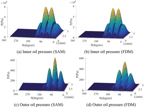
Figure 6 illustrates that the oil film pressure distributions calculated by the two methods are almost the same under different eccentricity ratios. Combined with Table 2, it can be seen that the errors of results calculated by the two methods increases with increasing eccentricity ratio, but all errors were found to be smaller than 4%, which is still within the error tolerance.

Figure 6. Inner oil pressure calculated by FDM and SAM, respectively, under different eccentricity ratios ε, for the case μ = 18 cP, ω = 91.8 Hz, ϕ = 0.5π, C₁ = 0.5 mm, C₂ = 0.5 mm, and L = 5 mm.

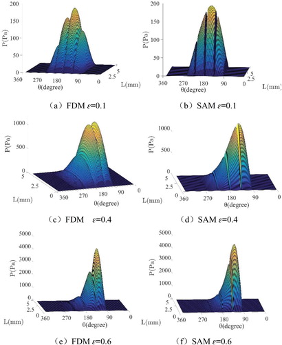
Table 2. Inner oil film pressure under different eccentricity ratios ε for the case μ = 18 cP, ω = 91.8 Hz, ϕ = 0.5π, C₁ = 0.2 mm, C₂ = 0.5 mm, and L = 5 mm.

		$\epsilon$
		0.1	0.2	0.3	0.4
P-max (Pa)	FDM	162	370.3	668.4	1160.7
	SAM	163.7	373.8	687.8	1224.7
ER (%)		1.00	0.90	2.82	5.20
ϕ-max (degrees)	FDM	165	151	148.1	127
	SAM	165	151	144.4	133
L-max (mm)	FDM	2.64	2.64	2.64	2.64
	SAM	2.64	2.64	2.64	2.64
Time (s)	FDM	4.33	4.16	4.15	4.2
	SAM	0.17	0.112	0.113	0.151
ER (%)		96.10	97.30	97.28	96.40

Figure 7 depicts the fact that the distributions of oil pressure with different precessional angles calculated by the two methods are almost the same. Combined with Table 3, it is clear that the error between maximum oil film pressures calculated by the two different methods do not change with a change in precessional angle, which is 5.2%. Figure 8 shows the oil film pressures with different axial lengths calculated by SAM and FDM. Combined with Table 4, it is clear that using moderately large axial lengths increases the relative errors of various oil pressures calculated by the above two methods. The reason is that, as the short bearing assumption is adopted for SAM, the computational error will rise significantly when the axial length-to-diameter ratio, L/2R, is not small enough. For example, when the axial length equals 10 mm, i.e. L/2R = 0.125, the error will be 12%.

Figure 7. Inner oil film pressure calculated by FDM and SAM, respectively, under different precessional angles ϕ, for the case μ = 18 cP, ε = 0.3, ω = 91.8 Hz, ϕ = 0.5π, C₁ = 0.5 mm, and C₂ = 0.5 mm.

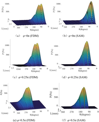
Figure 8. Inner oil film pressure calculated by FDM and SAM, respectively, under different axis lengths L for the case μ = 18 cP, ε = 0.4, ω = 91.8 Hz, ϕ = 0.5π, C₁ = 0.5 mm, and C₂ = 0.5 mm.

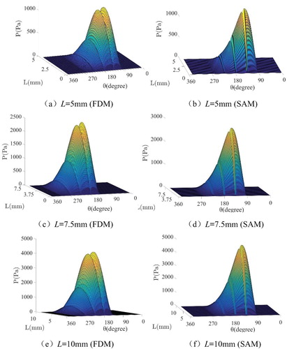
Table 3. Inner oil film pressure under different precessional angles ϕ for the case μ = 18 cP, ε = 0.3, ω = 91.8 Hz, C₁ = 0.5 mm, and C₂ = 0.5 mm.

		$\theta$
		0 π	0.25π	0.5π	0.75π
P-max (Pa)	FDM	668.4	668.4	668.4	668.4
	SAM	687.8	687.8	687.8	687.8
ER (%)		2.82	2.82	2.82	2.82
ϕ-max (degrees)	FDM	58.1	103.1	148.1	193.1
	SAM	54.4	99.4	144.4	189.3
L-max (mm)	FDM	2.64	2.64	2.64	2.64
	SAM	2.64	2.64	2.64	2.64
Time (s)	FDM	4.33	4.26	4.11	4.21
	SAM	0.17	0.13	0.12	0.15
ER (%)		96.10	96.94	97.08	96.44

Table 4. Inner oil film pressure under different axial lengths L for the case μ = 18 cP, ε = 0.4, ω = 91.8 Hz, ϕ = 0.5π, C₁ = 0.5 mm, and C₂ = 0.5 mm.

		L
		5 mm	7.5 mm	10 mm	12.5 mm
P-max (Pa)	FDM	1160.7	2495.1	4202	6176
	SAM	1224.7	2755.5	4898.7	7654
ER (%)		5.20	9.45	14.22	19.31
ϕ-max (degree)	FDM	148.1	150	153.7	153.7
	SAM	144.4	144.4	144.4	144.4
L-max (mm)	FDM	2.64	3.9	5.3	6.6
	SAM	2.64	3.9	5.3	6.6
Time (s)	FDM	4.15	4.25	4.15	4.46
	SAM	0.113	0.112	0.113	0.12
ER (%)		97.20	97.40	97.2	97.30

Because there is no iterative process in SAM, the computing time of SAM is reduced by more 96% compared with that of FDM in the above two cases. Although the accuracy of FDM increases with the grid density, the slow convergence will spend an amount of computing resource for the larger number of grids. In contrast, SAM is still efficient even when the number of grids is large (Table 5).

3.2. Damping and mass coefficients of the inner oil film

According to the references Han et al. (2019), San Andrés et al. (2015), San Andrés and Delgado (2007), and Jeung (2013), the cross damping and mass effects in the damper can be ignored. Equations (14) are used to calculate the inner oil dynamic characteristics at different equilibrium positions as shown in Figure 9. To ensure that the rotating journal arrives at an equilibrium position eventually, different loads should be added on the z₁- and y₁-directions in Equations (12), respectively. (14) $\begin{array}{rl}{M}_{zz}& =-\frac{1}{{\omega }^2}Re\left(\frac{\overline{F_z}}{\overline{z}}\right)C_{zz}=\frac{1}{\omega }\mathrm{Im}\left(\frac{\overline{F_z}}{\overline{z}}\right)\\ M_{yy}& =-\frac{1}{{\omega }^2}Re\left(\frac{\overline{F_y}}{y}\right)C_{yy}=\frac{1}{\omega }\mathrm{Im}\left(\frac{\overline{F_y}}{y}\right)\end{array}$(14)

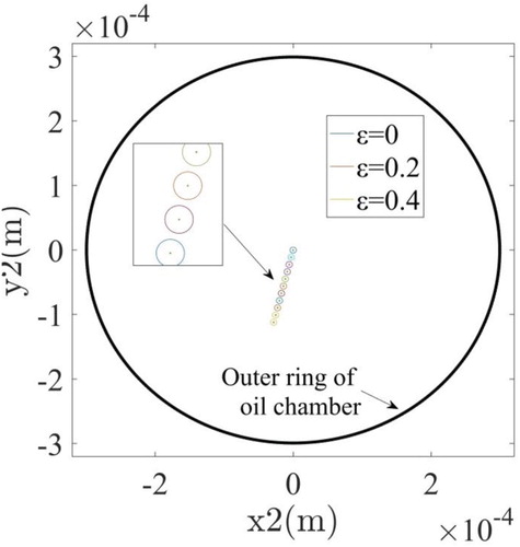
Figure 9. Equilibrium positions and precession trajectories of journal at different eccentricity ratios.

Variations of the oil inertia and damping coefficients in the ERSFD with increasing eccentricity, determined by SAM and FDM, are depicted in Figure 10. It can be shown that the oil damping and mass coefficients calculated by the two methods have the same growth trend with increasing eccentricity ratio, whereas the numerical difference errors are quite small. Thus, SAM is suitable for calculating oil film damping and mass.

Figure 10. Inner oil damping and mass coefficients of ERSFD for the case μ = 16 cP, ω = 64.5 Hz, C₁ = 0.3 mm, C₂ = 0.5 mm, L = 5 mm, and e_u = 8×10⁻⁸ m.

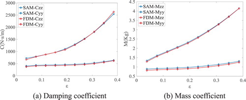
Table 5. Inner oil film pressure under different grid numbers for the case μ = 18 cP, ε = 0.3, ω = 91.8 Hz, ϕ = 0.5π, C₁ = 0.5 mm, C₂ = 0.5 mm, and L = 5 mm.

Grid	Number	$48\times 9$	$96\times 18$	$192\times 36$
P-max (Pa)	FDM	659	670	668.4
(Pa)	SAM	703	700	687.8
ER (%)		6.26	4.29	2.82
ϕ-max	FDM	157.5	150	148.1
(degree)	SAM	150	142.7	144.4
L-max	FDM	6	10	19
(mm)	SAM	6	10	19
Time	FDM	0.26	0.52	4.15
(s)	SAM	0.097	0.102	0.113
ER (%)		62.7	80.30	97.2

3.3. Amplitude–frequency relations of a linearized ERSFD supported rotor system

To investigate the influence of oil coefficients in an ERSFD-rotor, the amplitude–frequency relation of the linearized ERSFD-supported rotor system is assessed in this section. Using SAM, we analyse the dynamic time history of an ERSFD supported rotor system and the corresponding linearized oil damping coefficient. Then the system damping ratio, amplitude amplification factor, and phase difference under an equilibrium position (Thomson, 1988) are determined by (15) $\begin{array}{rl}{B}_{qi}& =\frac{1}{\sqrt{{\left(1+{\lambda }_i^2\right)}^2+{\left(2{\lambda }_i{\xi }_i\right)}^2}},\\ {\xi }_i& =\frac{C_{Pii}}{2P_{ni}\cdot M_{Pii}}\left(i=1,2\right),\tan {\varphi }_i=\frac{2{\lambda }_i{\xi }_i}{1-{\lambda }_i^2},\end{array}$(15) where B_qi, ξ_i and λ_i are the ith AAF, damping ratio, and frequency ratio, and P_ni is the ith natural frequency, respectively.

Because the z- and y-directions of the dynamic model are independent of each other, Equations (11) are simplified to (16) $\mathbf{\text{M}}\ddot{A}\text{ + }\mathbf{\text{CA}}\text{ + }\mathbf{\text{K}}\ddot{A}\text{ = }\mathbf{\text{F}}$(16) where $\begin{array}{r}{\lambda }_i=\frac{\omega }{p_{ni}},{\mathbf{\text{C}}}_{\mathbf{\text{P}}}{\mathbf{\text{= A}}}_{\mathbf{\text{P}}}^{\mathbf{\text{T}}}\mathbf{\text{C}}{\mathbf{\text{A}}}_{\mathbf{\text{P}}}=\left[\begin{array}{cc}{C}_{P11}& C_{P12}\\ C_{P21}& C_{P22}\end{array}\right],\\ {\mathbf{\text{M}}}_{\mathbf{\text{P}}}{\mathbf{\text{=}}A}_{\mathbf{\text{P}}}^{\mathbf{\text{T}}}\mathbf{\text{M}}{\mathbf{\text{A}}}_{\mathbf{\text{P}}}=\left[\begin{array}{cc}{M}_{P11}& M_{P12}\\ M_{P21}& M_{P22}\end{array}\right]\end{array}$ $\begin{array}{r}\mathbf{\text{F}}\text{ = }\left[\begin{array}{cc}{m}_1{\omega }^2{e}_u\cos \left(\omega t\right)& \text{0}\\ \text{0}& \text{0}\end{array}\right]\text{,}\mathbf{\text{M}}\text{ = }\left[\begin{array}{cc}{m}_1& \text{0}\\ \text{0}& m_2\end{array}\right],\\ \mathbf{\text{C}}\text{ = }\left[\begin{array}{cc}c& c_{12}\\ c_{21}& c_{\text{oil}}+c\end{array}\right],\mathbf{\text{A}}\text{ = }\left[\begin{array}{c}{z}_1\\ z_2\end{array}\right]\end{array}$ where A_p, C, F, K, and C_P are the principal mode, damping, stiffness, excitation, and regular damping matrices, respectively. ϕ_i is the phase difference between the response and excitation at the ith natural frequency. Assuming the cross damping parameters c₁₂ and c₂₁ are null. C_oil = F_θ/(Ωe) is the directly linearized oil film damping of ERSFD (Zhang & Ding, 2015), and c is the equivalent linear damping of the rotor system. The 1st and 2nd natural frequencies are determined by (17) $\begin{array}{rl}P{n}_1& =\sqrt{\frac{E_1-\sqrt{2E_1^2-16E_2}}{4m_1{m}_2}},\\ P{n}_2& =\sqrt{\frac{E_1+\sqrt{2E_1^2-16E_2}}{4m_1{m}_2}}\end{array}$(17) where E₁ = 2k₁m₂+2k₂m₁+k₁m₁ and E₂ = 16m₁m₂k₁k₂.

It can be seen from the amplitude–frequency relations as shown in Figure 11(a) that the AAF of the linear damping system with damping coefficient c reaches its maximum, about 16, at the first natural frequency. Figure 11(b) reveals that the damping ratio of the linear damping system remains at about 0.03 during the whole process. Correspondingly, the AAF of the ERSFD system is rapidly suppressed around the natural frequency, which indicates the amplitude of the system is significantly reduced. The reason is that the large precessional amplitude of the bushing near the natural frequency will cause the oil film of the ERSFD to be sufficiently squeezed, thus more damping and mass effect of the damper are provided to enhance the damping ratio of the system. The mechanism of this phenomenon is like the tuned mass damper (TMD) introduced in detail in Dresig and Holzweißig (2016). While not near the natural frequency, the damping ratio of the ERSFD-rotor system remains almost constant but is still bigger than that of the linear damping rotor system.

Figure 11. AAF and damping ratio of an ERSFD supported rotor and a linear rotor without a damper for μ = 4 cP, C₁  =  0.2 mm, C₂ = 0.5 mm, L = 5 mm, c = 200 N·s·m⁻¹, and e_u = 2.5×10⁻⁵m.

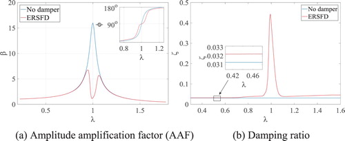
In the inset in Figure 11(a), i.e. the phase difference diagram, one finds that there is a damping speed region where the phase difference is around 90° near the first natural frequency in the ERSFD-rotor system. This means that the damping region in the ERSFD-rotor system where the damping plays a major role to suppress the vibration is bigger than the region in the linear damping system. In other words, the ERSFD makes the rotor system more stable.

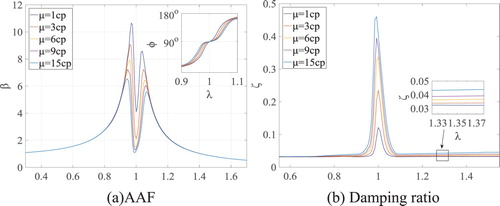
Figure 12 indicates the influence of oil viscosity on the amplitude–frequency characteristics of the rotor supported on ERSFDs whose axial length L = 5 mm, elastic ring stiffness k_e = 4.21×10⁴ N·m⁻¹, and number of inner and outer bosses is four, respectively. The higher oil viscosity effectively multiplies the damping ratio and damping region, lowering the AAF, and giving a greater region where AAF is reduced. Therefore, oil of higher viscosity is beneficial for vibration suppression in the ERSFD-rotor system.

Figure 12. AAF and damping ratio of a linearized ERSFD supported rotor system with different oil viscosities μ for C₁ = 0.3 mm, C₂ = 0.5 mm, L = 5 mm, c = 200 N·s·m⁻¹, and e_u = 3.67×10⁻⁵ m.

4. Dynamic response

By comparing the dynamic responses of the ERSFD-rotor system obtained by SAM with numerical (Han et al., 2019) and experimental results, the accuracy of SAM is verified in this section. Then the dynamic responses of the SFD-rotor and the ERSFD-rotor sweeping up and down at the 1st resonance are simulated by SAM in Section 4.2. The responses of the ERSFD-rotor system and the rotor without a damper system under sudden unbalanced excitation are analysed in Section 4.3.

4.1. Amplitude–frequency characteristics in first-order resonance

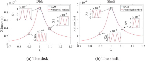
The time histories of vibration at the disk and one shaft end are presented in Figure 13. Comparison between the results calculated by SAM (blue line) and the numerical method (red line) indicates that the difference is quite small, with about 5% maximum relative error appearing at the resonant frequency. Meanwhile, the calculation time of SAM is 317.1 s, which is more than 96% shorter than that of the numerical method, 8734.7 s.

Figure 13. Dynamic responses obtained by semi-analytic and numerical methods, respectively, for the case μ = 5 cP, C₁ = 0.8 mm, C₂ = 0.2 mm, L = 20 mm, c = 200 N·s·m⁻¹, and e_u = 0.94×10⁻⁴ m.

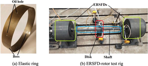
To verify the results of SAM further, the rotor test rig supported by two ERSFDs and bearing mouse cages, depicted in Figure 14, was built. Figure 14(a) illustrates the elastic ring with four inner and outer bosses, respectively. The ERSFDs, antifriction bearing, and mouse cage are assembled at both sides as shown in Figure 14(b). The motor used to drive the shaft develops about 400 W at a top running speed of 4000 rpm. Making use of four eddy current sensors placed at the disk and the right end of the shaft, respectively, we can pick up the vertical and horizontal vibrations of the disk and bushing, i.e. journal.

Figure 14. ERSFD-rotor test rig.

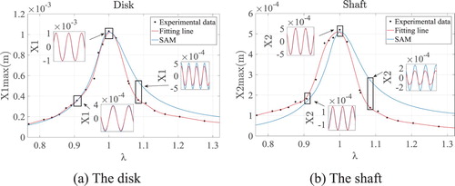
Using the parameters listed in Table 1, we find that the primary resonance happens as the precession frequency approaches the 1st natural frequency (51.76 Hz) of the rotor. The resonant amplitude–frequency curves, obtained by SAM (the blue lines) and experiment (the black points and the fitting line), are presented in Figure 15. The inset shows the time histories of vibration at specific frequencies. Clearly, the peak of the dynamic response appears at the frequency ratio λ = 1. The difference between the amplitude peaks calculated by the two methods is about 3%, whereas the difference between the amplitudes becomes greater when λ differs to a greater extent from one, but still remains inside 30%. The main reason causing this phenomenon is the inherent error between the Jeffcott rotor model and the actual rotor model. Furthermore, the difference is also caused by the placement of the eddy sensors, which cannot be completely installed at the end of the shaft because of size limitations, thus the error at the end of the shaft is bigger than that at the disk.

Figure 15. Dynamic responses obtained by SAM and experiment, respectively, for the case μ = 5 cP, C₁ = 0.8 mm, C₂ = 0.2 mm, L = 20 mm, c = 200 N·s·m⁻¹, and e_u = 0.93×10⁻⁵ m.

Although there are inevitable differences between the results obtained by the above three methods, SAM calculates the dynamic response accurately and reduces the calculated time significantly. Therefore, SAM is used to analyze the bi-stable response in the next section.

4.2. Bi-stable responses of SFD and ERSFD-rotors

Figure 16 shows the amplitude of the SFD-system and the ERSFD-system under the same unbalanced distance e_u and the same oil film thickness. The vibration amplitudes of disk D₁ and end of shaft D₂ are obtained by (18) $D_1=\sqrt{x_1^2+y_1^2},D_2=\sqrt{x_2^2+y_2^2}$(18)

Figure 16. Dynamic response of a four-boss ERSFD-rotor system and an SFD-rotor system calculated by SAM for e_u = 7.3×10⁻⁶ m, C₁ = 0.3 mm, C₂ = 0.3 mm, L = 5 mm, and c = 20 N·s·m⁻¹.

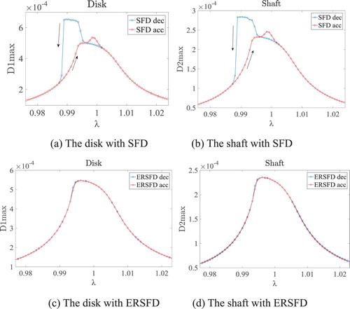
Note that for most of the precession frequency range in Figures 16(a) and 16 (b), the rotor could rotate at the same amplitude whether the frequency sweeps up or down. Further, increasing the amplitude of the journal causes a rapid raise in nonlinearity of the equivalent oil stiffness in the SFD when λ approaches 0.99 and 1. Hence, as the frequency ratio decreases, the amplitude increases through the peak at λ = 0.99 and subsequently crashes to the low-amplitude curve. More interestingly, if the speed sweeps up, there is no obvious jump at around λ = 0.99. This reveals that there are two steady states of the rotor depending on different initial conditions under the same excitation frequency. That is a bi-stable response, a typical vibration phenomenon for nonlinear systems. This refers to the soft-support stiffness in the SFD-rotor, which can cause harmful damage to the rotor system. No analogous phenomenon is found in the ERSFD-rotor system. In other words, the level of nonlinear oil stiffness in the damper is reduced by the elastic ring.

4.3. Response of the ERSFD-rotor under sudden unbalanced excitation

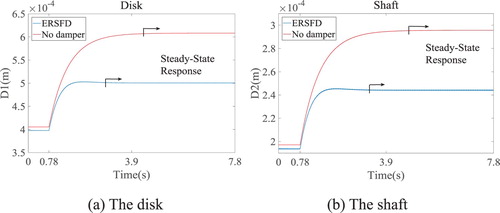
In engineering practice, blade loss caused by bird strike, fatigue, overstress, or corrosion always generates a sudden unbalanced excitation, Δe_u, on the rotor, which may damage the rotating machinery (Huang & Wang, 2020; Zhou et al., 2014). The sudden unbalanced responses of the ERSFD-rotor and the rotor without a damper are simulated by SAM, as shown in Figure 17. By comparison with the linear damping rotor system without a damper, ERSFD leads the rotor to reach a steady-state more quickly. Additionally, the vibration amplitude of the ERSFD-rotor is much smaller than that of the rotor without a damper. That means that the ERSFD can provide more damping effect to suppress large vibrations of the rotor caused by sudden excitation and ensure that the device works properly.

Figure 17. Time histories of a four-boss ERSFD-rotor system and a rotor without a damper system under sudden excitation: Δe_u = 1.67×10⁻⁶ m and c = 20 N·s·m⁻¹ for e_u = 3.8×10⁻⁶ m, C₁ = 0.4 mm, δ = 0.5 mm, C₂ = 0.5 mm, and L = 5 mm.

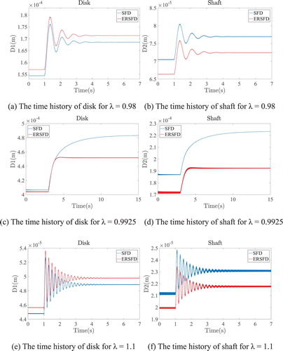
To investigate further the abilities of SFD and ERSFD in restraining the sudden unbalanced response when the rotor system has a ‘jump’ phenomenon (Figure 16), the time histories of two systems are calculated. It can be seen that, in the non-jump area such as ‘λ = 0.98’ as shown in Figures 18(a) and 18(b), and ‘λ = 1.1’ as shown in Figures 18(e) and 18(f), due to the oil film damping and the mass of the dampers being small, there are obvious transient vibration processes with significant peaks in both systems. Since the elastic ring increases the support stiffness of the rotor, the transient vibration peak in the SFD-rotor at the end of the shaft is bigger than that in the ERSFD-rotor, while the transient vibration peak in the SFD-rotor at the disk is smaller than that in the ERSFD-rotor. In contrast, because the oil film damping and the mass of the two types of damper are quite a lot bigger in the jump area, there are no obvious transient processes with vibration peaks found in the ERSFD-rotor and the SFD-rotor as shown in Figures 18(c) and 18(d). Moreover, the nonlinear effect of the oil film becomes strong when a jump phenomenon occurs in the SFD-rotor system, hence the system has a bi-stable response that makes the amplitudes at the end of the shaft and the disk bigger than those in the ERSFD–rotor. From the above two cases, it is instructive to see that ERSFD makes a rotor influenced by a sudden excitation become more stable.

Figure 18. Time histories of a four-boss ERSFD-rotor system and an SFD-rotor system under sudden excitation: μ = 5 cP, Δe_u = 0.67×10⁻⁶ m for e_u = 7.3×10⁻⁶ m, C₁ = 0.3 mm, C₂ = 0.3 mm, L = 5 mm, and c = 20 N·s·m⁻¹.

5. Conclusions

This paper proposes a semi-analytical method (SAM) for analyzing the dynamic characteristics of an ERSFD supported rotor system. The short bearing and π-film assumptions are used in this paper. In practice, cavitation in ERSFD is a complicated phenomenon. Hence, a future analysis of the cavitation effect on the dynamic characteristics of ERSFD would be helpful for engineering design. Although the analysis presented above has several limitations, it does obtain a number of useful results.

First, SAM is verified by numerical and experimental comparisons. Because the dynamic analysis of the ERSFD supported rotor requires calculation of the oil pressure twice at each time step, SAM is able to reduce the overall computing time of the previous numerical method by more than 90% at the same level of accuracy. In practice, the improved calculation time of SAM is the foundation for the optimization of ERSFD and complicated dynamic analyses of, for example, the influence of multiple dampers, misalignment, and flight maneuvers. If the ratio of the axial length to diameter is large, the general principle of SAM can be extended to the long-bearing assumption.

Secondly, by analyzing the amplitude–frequency relations of a linearized ERSFD-supported rotor system, we find that ERSFD can increase the stability of the system in the following two aspects. First, the damping ratio of the rotor system can be increased by ERSFD, especially when the precession speed approaches the 1st natural frequency. For this reason, the AAF of the system is significantly reduced. Secondly, ERSFD is able to increase the damping region to weaken the influence of oil film stiffness and inertia effects on the rotor system.

Finally, the dynamic responses of the ERSFD-rotor system, the SFD-supported rotor system, and the rotor system without a damper, all under sudden unbalanced excitation, are analyzed by SAM. The results indicate that ERSFD is able to maintain a more stable rotor system, thus the transient amplitude peak under sudden excitation is significantly reduced and there is no jump phenomenon in the ERSFD-rotor system.

Disclosure statement

No potential conflict of interest was reported by the authors.

Additional information

Funding

This work was supported by the National Natural Science Foundation of China [Grant Number 51575378]; the Natural Science Foundation of Tianjin City [Grant Number 19JCZDJC38800].

References

- Abed, A., Bouzidane, A., Thomas, M., & Zahloul, H. (2017). Performance characteristics of a three-pad hydrostatic squeeze film damper compensated with new electrorheological valve restrictors. Proceedings of the Institution of Mechanical Engineers, Part J: Journal of Engineering Tribology, 231(7), 889–899. https://doi.org/10.1177/1350650116683622
- Akbarian, E., Najafi, B., Jafari, M., Faizollahzadeh Ardabili, S., Shamshirband, S., & Chau, K. (2018). Experimental and computational fluid dynamics-based numerical simulation of using natural gas in a dual-fueled diesel engine. Engineering Applications of Computational Fluid Mechanics, 12(1), 517–534. https://doi.org/10.1080/19942060.2018.1472670
- Bangchun, W., Jialiu, G., Songbo, X., Zheng, W., Jun, Z., Wen, Z., Jiajun, Qiu, Q., Taiping, H., Zhengsong, Z., & Wei, G. (2000). Advanced rotor dynamics (1st ed.). China Machine Press.
- Boyaci, A. L., Lu, D., & Schweizer, B. (2015). Stability and bifurcation phenomena of Laval/Jeffcott rotors in semi-floating ring bearings. Nonlinear Dynamics, 79(2), 1535–1561. https://doi.org/10.1007/s11071-014-1759-5
- Changsheng, Z., & Xixuan, W. (1995). An experimental investigation on the effectiveness of advanced hybrid squeeze film damper. Journal of Vibration Engineering, 8(3), 281–285.
- Chen, H., Chen, Y., Hou, L., & Li, Z. (2014). Bifurcation analysis of rotor–squeeze film damper system with fluid inertia. Mechanism and Machine Theory, 81(8), 129–139. https://doi.org/10.1016/j.mechmachtheory.2014.07.002
- Chen, H., Hou, L., Chen, Y., & Yang, R. (2016). Dynamic characteristics of flexible rotor with squeeze film damper excited by two frequencies. Nonlinear Dynamics, 87(4), 1–19. https://doi.org/10.1007/s11071-016-3204-4
- Dresig, H., & Holzweißig, F. (2016). Maschinendynamik. Springer-Verlag Berlin Heidelberg.
- Ghalandari, M., Bornassi, S., Shamshirband, S., Mosavi, A., & Chau, K. W. (2019). Investigation of submerged structures’ flexibility on sloshing frequency using a boundary element method and finite element analysis. Engineering Applications of Computational Fluid Mechanics, 13(1), 519–528. https://doi.org/10.1080/19942060.2019.1619197
- Guan, X., Zhou, J., Jin, C., Xu, Y., & Cui, H. (2019). Influence of different operating conditions on centrifugal compressor surge control with active magnetic bearings. Engineering Applications of Computational Fluid Mechanics, 13(1), 824–832. https://doi.org/10.1080/19942060.2019.1639216
- Han, B., & Ding, Q. (2018). Forced responses analysis of a rotor system with squeeze film damper during flight maneuvers using finite element method. Mechanism and Machine Theory, 122, 233–251. https://doi.org/10.1016/j.mechmachthe-ory.2018.01.004
- Han, Z., Ding, Q., & Zhang, W. (2019). Dynamical analysis of an elastic ring squeeze film damper-rotor system. Mechanism and Machine Theory, 131, 406–419. https://doi.org/10.1016/j.mechmachtheory.2018.10.011
- Holmes, R. (1972). The non-linear performance of squeeze film bearings. Journal of Mechanical Engineering Science, 14(1), 74–77. https://doi.org/10.1243/JMES_JOUR_1972_014_011_02
- Hou, L., Chen, H., Chen, Y., Lu, K., & Liu, Z. (2019). Bifurcation and stability analysis of a nonlinear rotor system subjected to constant excitation and rub-impact. Mechanical Systems and Signal Processing, 125, 65–78. https://doi.org/10.1016/j.ymssp.2018.07.019
- Hou, L., Chen, Y., Fu, Y., Chen, H., Lu, Z., & Liu, Z. (2017). Application of the HB–AFT method to the primary resonance analysis of a dual-rotor system. Nonlinear Dynamics, 88(4), 2531–2551. https://doi.org/10.1007/s11071-017-3394-4
- Huang, J., & Wang, Y. (2020). Transient analysis for a twin spool rotor with squeeze-film dampers considering blade loss. Journal of Vibration Engineering & Technologies, 8(1), 95–104. https://doi.org/10.1007/s42417-018-0060-1
- Jeung, S. H. (2013). Performance of an open ends squeeze film damper operating with large amplitude orbital motions: Experimental analysis and assessment of the accuracy of the linearized force coefficients model. Master's thesis, Texas A&M University. http://hdl.handle.net/1969.1/151648.
- Jie, H., Yin, D., & Dayi, Z. (2006). Dynamic design method of elastic ring squeeze film damper. Journal of Beijing University of Aeronautics and Astronautics, 32(6), 649–653.
- Karimulla, S., Dutta, B. K., & Gouthaman, G. (2019). Experimental and analytical investigation of short squeeze-film damper (SFD) under circular-centered orbit (CCO) motion. Journal of Vibration Engineering & Technologies, 8, 215–224. https://doi.org/10.1007/s42417-019-00100-9
- Lei, C. (2006). Theoretical and experimental study on dynamic characteristics of combined elastic support-damper. Nanjing University of Aeronautics and Astronautics.
- Min, Z., Qihan, L., & Litang, Y. (1998). Study on vibration reduction and mechanism of an elastic ring damper(1). Gas Turbine Experiment and Research, 1(4), 19–23.
- Salih, S. Q., Aldlemy, M. S., Rasani, M. R., Ariffin, A. K., Ya, T. M. Y. S., Al-Ansari, N., Yaseen, Z. M., & Chau, K. W. (2019). Thin and sharp edges bodies-fluid interaction simulation using cut-cell immersed boundary method. Engineering Applications of Computational Fluid Mechanics, 13(1), 860–877. https://doi.org/10.1080/19942060.2019.1652209
- San Andrés, L., & Delgado, A. (2007). Identification of force coefficients in a squeeze film damper with a mechanical end seal—centered circular orbit tests. Journal of Tribology, 129(3), 660–668. https://doi.org/10.1115/1.2736708
- San Andrés, L., Jeung, S. H., & Bradlet, G. (2015). Dynamic forced performance of short length open-ends squeeze film damper with end grooves. In Proceedings of the 9th IFToMM International Conference on Rotor Dynamics.
- San Andres, L., & Vance, J. M. (1988). Effect of fluid inertia on the performance of squeeze film damper supported rotors. Journal of Engineering for Gas Turbines and Power-Transactions of the ASME, 110(1), 51–57. https://doi.org/10.1115/1.3240086
- Siew, C. C., Hill, M., & Holmes, R. (2002). Evaluation of various fluid-film models for use in the analysis of squeeze film dampers with a central groove. Tribology International, 35(8), 533–547. https://doi.org/10.1016/S0301-679X(02)00048-8
- Thomson, W. T. (1988). Theory of vibration with applications (3rd ed.). Prentice-Hall.
- Wang, B., Ding, Q., & Yang, T. (2019). Soft rotor and gas bearing system: Two-way coupled fluid-structure interaction. Journal of Sound and Vibration, 445, 29–43. https://doi.org/10.1016/j.jsv.2019.01.007
- Wang, X., Han, Z., Ding, Q., & Zhang, W. (2018). Influence of fluid inertia on dynamic characteristics of elastic ring squeeze film damper-rotor system. Journal of Aerospace Power, 33(12), 2981–2990. https://doi.org/10.13224/j.cnki.jasp.2018.12.019
- Wang, Z., Ning, X., Xiangyu, Y., Zhansheng, L., & Guanghui, Z. (2017). The dynamic characteristic analysis of elastic ring squeeze film damper by fluid-stru cture interaction approach. In Proceedings of ASME Turbo Expo 2017: Turbomachinery Technical Conference and Exposition GT2017.
- Dai, X., & Wang, G. (1994). Analysis on stiffness of corrugated ring in a rotor-bearing support. Journal of Harbin Institute of Technology, 26(5), 40–43.
- Zhang, W., & Ding, Q. (2015). Elastic ring deformation and pedestal contact status analysis of elastic ring squeeze film damper. Journal of Sound and Vibration, 346, 314–327. https://doi.org/10.1016/j.jsv.2015.02.015
- Zhang, J., Ellis, J., & Roberts, J. B. (1993). Observations on the nonlinear fluid forces in short cylindrical squeeze film dampers. Journal of Tribology, 115(4), 692–698. https://doi.org/10.1115/1.2921695
- Zhou, H., Feng, G., Luo, G., Ai, Y., & Sun, D. (2014). The dynamic characteristics of a rotor supported on ball bearings with different floating ring squeeze film dampers. Mechanism and Machine Theory, 80, 200–213. https://doi.org/10.1016/j.mechmachtheory.2014.04.016
- Zhu, C. S., Robb, D. A., & Ewins, D. J. (2002). Analysis of the multiple-solution response of a flexible rotor supported on non-linear squeeze film dampers. Journal of Sound and Vibration, 252(3), 389–408. https://doi.org/10.1006/jsvi.2001.3910