Flow features in a pooled fishway with V-shaped weir formation

ABSTRACT

A pooled fishway is an artificial structure to improve the river flow connectivity and facilitate fish migration. Its conventional layout is characterized by straight weirs and suffers from limited passage rate. To improve its flow behaviors, an alternative design, featuring a V-shaped weir arrangement, is devised. CFD simulations are performed to examine its effects on the flow conditions. The governing geometrical parameters include weir angling, height, and spacing. Depending on weir arm angle, the flow is directed towards either the channel’s central part or the sidewalls, leading to both across- and along-channel differences in flow velocity and turbulent kinetic energy. This offers conducive zones for multiple fish species with distinct swimming preferences. For a given location in a pool, the cross-sectional velocity exhibits a cosine-type variation; a relationship is established to predict the maximum longitudinal velocity. The pressure distribution exhibits a similar pattern, with high-pressure areas residing upstream of the weir. A power law describes the relationship between the energy dissipation rate and unit discharge with an exponent at approximately 2/3. With an increase in either weir spacing or height, the energy dissipation rate declines. A change in weir angle shows however a negligible influence on it.

KEYWORDS:

• Pooled fishway
• conventional layout
• V-shaped weir
• flow feature
• CFD

1. Introduction

As a renewable energy source, the past decades have seen constructions of a growing number of hydropower facilities (Jackson & Marmulla, 2001; Nilsson et al., 2005). However, the environmental impacts they generate have become an issue of concern for many rivers. A dam on a river prevents fish species from migration upstream, resulting in their drastic decrease in number or even extinction (Kubečka et al., 1997; Larinier, 2001). In order to mitigate the adverse effect, a fish passage is introduced to assist the fish to navigate through the obstacles (Clay, 2017; Katopodis, 2005). As a commonly used fish passage in small projects (Alvarez-Vázquez et al., 2008; Larinier, 2008), the pool and weir fishway features a series of pools formed by cross-walls (weirs) in the waterway (Katopodis et al., 2001). The structure, easy to construct and maintain, has gained popularity in research and practice (Katopodis, 2005). The pools and weirs increase the energy loss and reduce the flow velocity. The low velocity at a weir allows the target species to navigate upstream; the pool offers a resting area if the velocity is less than their cruising speed (Clay, 2017; Larinier, 2002a). Depending on the fishway geometry and flow condition, the flow regimes in a pooled fishway are classified into plunging, transitional, streaming and supercritical jet flows (Ead et al., 2004; Santos et al., 2012).

Some limitations exist, however, in this conventional type of fishway. One drawback is that the along-channel spatial fluctuations, significant in many cases, in water-surface level are unfavorable for migration (Katopodis, 1992). To address this issue, modifications are necessary to augment the fish passage efficiency. Kim (2001) finds that a pool-weir fishway with a notch in a straight configuration creates a more suitable resting area than the one with a zigzag pattern. Rajaratnam et al. (1989) propose a pool-orifice fishway, in which a vertical slot and a submerged jet regime are identified. Studies by Branco et al. (2013) suggest that incorporating surface notches into the weirs facilitate, on one hand, surface-oriented species in their upstream migration in the streaming portion of flow. The orifices and notches require, on the other hand, frequent maintenance, as they are likely to be clogged by debris (FAO, 2002). Another disadvantageous aspect of the conventional pool-weir fish pass (without notches and orifices) is that it is suitable only for specific species (Katopodis et al., 2001; Yagci, 2010). Because the weirs are a thin plate, without any spanwise variation, the resulting flow pattern is typically two-dimensional.

A non-liner weir design is an option to mitigate the above-mentioned deficiencies. For instance, Kupferschmidt and Zhu (2017) suggest that, in a natural fishway, the use of V-shaped boulder weirs produces three-dimensional (3D) flow motions and offers significant advantages in assisting multispecies fish migration. A notch installed in the V-shaped rock-weir leads to a 20% increase in the maximum flow velocity and a 7% decrease in water depth (Baki et al., 2017a). Although there are studies on improvements in weir design of rock-weir fish passes, few has focused on the technical type fishways. The effects of weir layout on the flow features are not well understood.

A novel fish pass structure with a V-shaped weir layout on the plan view is devised. The investigation is made with the help of numerical modeling, which is commonly used in solving engineering problems (Pan et al., 2017; Pan & Wang, 2020). For instance, Mosavi et al. (2019) study the multi-inputs bubble column reactor using computational fluid dynamics (CFD) and machine learning approaches. Salih et al. (2019) develop a cut-cell immersed boundary method for simulations of flows at the fluid-structure interface for thin objects. Ghalandari et al. (2019) combine a boundary element and finite element methods to investigate the sloshing in tanks with flexible submerged structures. For fishway studies, numerical methods are also an efficient tool in examinations of the hydraulic behaviors (Baki et al., 2017b , Chorda et al., 2010, Katopodis, 2015, Khan, 2006, Puertas et al., 2012, Wang et al., 2010). The present numerical model is verified against the experimental data from the conventional fishway tested by Ead et al. (2004). The modeling emphasis is laid on the weir arrangement, in which the governing geometrical parameters are varied. The research aims to improve hydraulic conditions of the conventional fishway and facilitate upstream migration, whereby references are provided for engineering applications.

2. Fishway layouts

A V-shaped weir, similar to a unit in a labyrinth weir, is a common structure for flow diversion in irrigation, land drainage and urban sewage systems (Coşar and Agaccioglu, 2004, Ghodsian, 2004). In fish passages, its use is limited. Previous studies focus mainly on its features of discharge capacity (Emiroglu et al., 2010, Kisi et al., 2012). Compared with a single one, interconnected weirs might exhibit different, perhaps improved flow behaviors. In this study, a series of V-shaped weirs are designed for vertical placement in a fishway. Figure 1(a) illustrates the concept with three configurations:

• Layout I – V-shaped weirs with vertexes pointing downstream;

• Layout II – A conventional design with weirs normal to sidewalls and

• Layout III – V-shaped weirs with vertexes pointing upstream.

Figure 1. Schematics of fishway: (a) plan view of the proposed layouts, and (b) setup of laboratory model by Ead et al. (2004).

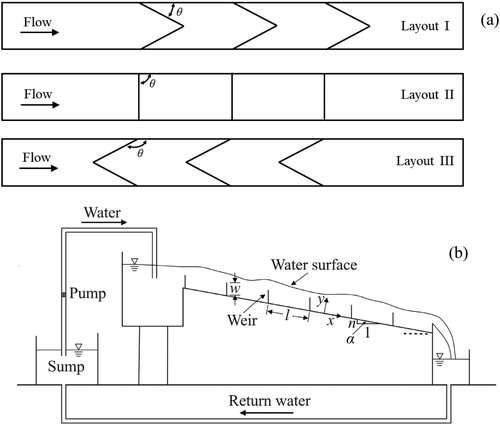
The weirs are placed symmetrically in cross-section. For a given layout, the primary geometrical parameters include the channel slope (α), weir height (w), weir width (B), weir spacing (l) and weir arm angle (θ). α is the channel-bottom sloping angle with the horizontal and θ refers to the angle of the weir arm with the sidewall downstream. Layouts I, II and III correspond to θ < 90°, = 90° and > 90°, respectively.

Ead et al. (2004) report a study of a conventional pool-and-weir fishway in an experimental rig [Figure 1(b)]. The test flume is placed between two water tanks and installed at a slope with n = tanα = 10%. The circulating water is pumped from the underground reservoir into the upper tank, in which an overflow side is installed to guarantee constant water stage. The flume is constructed with aluminum bottom and Plexiglas sidewalls, 600-cm long, 60-cm high and 56-cm wide. Flow rates in the rig are measured with a magnetic flowmeter, water-surface levels with point gauges and flow velocity with a propeller probe. The experimental arrangement and results are well documented, which is the reason why the study by Ead et al. (2004) is used as a basis for the CFD model calibration in our study.

In addition to the model calibration using Layout II, Layouts I and III are dimensioned to fit into the experimental flume. n remains unchanged and each weir covers the entire flume, i.e. B = 56 cm. The other three parameters, θ, w, and l, are changed, which are believed to have a bearing on the fishway flow conditions. The simulated cases are summarized in Table 1, with 13 cases of geometrical modifications. At given w and l values, Cases A1–A5 examine the effects of θ. At specified θ and l values, Cases B1–B4 compare the influences of w. Cases C1–C4 look into the impacts of l if θ and w are kept constant.

Table 1. List of simulated geometrical combinations.

Weir layout	Case no.	θ (°)	w (cm)	l (cm)
Layout I	A1	45	11.91	68.5
	A2	60
Layout II	A3	90
Layout III	A4	120
	A5	135
Layout III	B1	120	7.41	68.5
	B2		11.91
	B3		14.08
	B4		17.50
Layout III	C1	120	11.91	16.4
	C2			34.2
	C3			68.5
	C4			83.0

3. Numerical simulations

CFD modeling is performed to explore the hydraulic features of the fishway layouts. The k-ε turbulence model and the Volume of Fluid (VOF) method are combined to reproduce the flow behaviors. The simulations are made in three dimensions, covering the entire flume width. A (x, y, z) coordinate system is set up, with its origin (0, 0, 0) on the chute bottom and along the symmetry plane. Positive x points downstream in the flow direction and positive y upwards perpendicular to the channel bottom [Figure 1(b)].

3.1. Governing equations

Equivalent to physical model tests, numerical modeling is an effective way to study fishway hydraulics (Li et al., 2020, Marriner et al., 2014, Xu and Jin, 2014). Investigations (Baki et al., 2016, Baki et al., 2017b, Bombač et al., 2014, Naghavi et al., 2011) have indicated the robustness of the k-ε turbulence model. Its governing equations are as follows.

The turbulence kinetic energy (k) equation: (1) $\begin{array}{rl}& \frac{\mathrm{\partial }\left(\rho k\right)}{\mathrm{\partial }t}+\frac{\mathrm{\partial }}{\mathrm{\partial }{x}_i}\left(\rho u_{i}k\right)\\ & =\frac{\mathrm{\partial }}{\mathrm{\partial }{x}_i}\left[\left(\mu +\frac{{\mu }_t}{{\sigma }_k}\right)\frac{\mathrm{\partial }k}{\mathrm{\partial }{x}_i}\right]\\ & +G_k+G_b-\rho \epsilon -Y_M+S_k\end{array}$(1) The turbulence kinetic energy dissipation rate (ε) equation: (2) $\begin{array}{rl}& \frac{\mathrm{\partial }\left(\rho \epsilon \right)}{\mathrm{\partial }t}+\frac{\mathrm{\partial }\left(\rho u_i\epsilon \right)}{\mathrm{\partial }{x}_i}\\ & =\frac{\mathrm{\partial }}{\mathrm{\partial }{x}_i}\left[\left(\mu +\frac{{\mu }_t}{{\sigma }_{\epsilon }}\right)\frac{\mathrm{\partial }\epsilon }{\mathrm{\partial }{x}_i}\right]\\ & +C_{1\epsilon }\frac{\epsilon }{k}\left(G_k+G_{3\epsilon }{G}_b\right)-C_{2\epsilon }\rho \frac{{\epsilon }^2}{k}+S_{\epsilon }\end{array}$(2) in which ρ = water density, u_i = velocity component (i = x, y, z), t = time, μ = dynamic viscosity (= 10⁻³ Pa/s at 20°C), μ_t = turbulent dynamic viscosity, G_k = generation of turbulent kinetic energy due to mean velocity gradients, G_b = generation of turbulent kinetic energy due to buoyancy, Y_M = contribution of the fluctuating dilatation in compressible turbulence to the overall dissipation rate, σ_k, σ_ε = turbulent Prandtl numbers for k and ε, and S_k and S_ε = user-defined source terms. The default model constants are C_μ = 0.09, σ_k = 1.0, ε = 1.3, C_1ε = 1.44, C_2ε = 1.92, and C_3ε = 1.0.

In combination with the k-ε model, the VOF method is introduced to track the air–water interface in a cell, which is realized with the geometric reconstruction scheme. (3) $\begin{array}{r}\frac{\mathrm{\partial }{\alpha }_w}{\mathrm{\partial }t}+u_i\frac{\mathrm{\partial }{\alpha }_w}{\mathrm{\partial }{x}_i}=0\end{array}$(3) The continuity and momentum equations are (4) $\begin{array}{rl}\frac{\mathrm{\partial }\rho }{\mathrm{\partial }t}+\frac{\mathrm{\partial }\rho u_i}{\mathrm{\partial }{x}_i}& =0\end{array}$(4) (5) $\begin{array}{rl}\frac{\mathrm{\partial }\rho u_i}{\mathrm{\partial }t}+\frac{\mathrm{\partial }\rho u_i{u}_j}{\mathrm{\partial }{x}_j}& =-\frac{\mathrm{\partial }P}{\mathrm{\partial }{x}_i}+\frac{\mathrm{\partial }}{\mathrm{\partial }{x}_j}\left(\mu +{\mu }_t\right)\left(\frac{\mathrm{\partial }{u}_i}{\mathrm{\partial }{x}_j}+\frac{\mathrm{\partial }{u}_j}{\mathrm{\partial }{x}_i}\right)\end{array}$(5) in which α_w = volume fraction of water and P =pressure. The max. and min. values of α_w are 1 and 0, corresponding to full water and only air in a cell, respectively.

The simulations are performed in ANSYS Fluent. Based on the finite-volume method, the governing equations are solved with the SIMPLE algorithm for the coupling of pressure and velocity in a given cell (Caretto et al., 1973). For solutions of P and α_w, the PRESTO! and Geo-Reconstruct techniques are used (ANSYS Inc, 2019). The second-order upwind scheme is applied for the momentum; the first-order upwind scheme for the turbulent kinetic energy and dissipation rate.

3.2. Model verification

To demonstrate the reliability of the CFD model, the pool and weir fish passage from Ead et al. (2004) is established numerically (Figure 2). The computational domain with seven pools covers the whole flume width and height; it starts from the cross-section 1.5 l upstream of the first weir, and ends up at the cross-section 1.0 l downstream of the last weir. The domain is meshed with structured hexahedral grids, with denser cells around the weirs. The min. and max. size of the grid is 0.8 and 1.5 cm, respectively. Its top boundary is defined as pressure inlet; the downstream boundary (exit) is set as pressure outlet. The upstream boundary includes two parts: a velocity inlet of water from the bottom to the free water surface and a pressure inlet of air above the water surface. The sidewalls, bottom and weirs are treated as wall boundary (Figure 2). The Enhanced Wall Function is used. Table 2 summarizes the experimental parameters used for model calibration. Three cases, Tests 1, 2 and 3, are included, with combinations of w, l and Q, in which Q = flow rate in the channel.

Figure 2. Computational domain with boundary conditions.

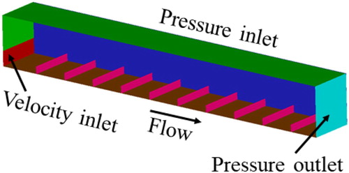
Table 2. Model calibration based on experiments by Ead et al. (2004).

Test no.	w (cm)	l (cm)	Q (litre/s)
1	7.4	68.5	35
2	14.1	68.5	35
3	14.1	33.5	65

The model verification includes grid sensitivity check and comparison with experimental results. The former is to guarantee grid-independent solutions. For the geometry in Test no. 2, three grid sets of varying density, denoted as Mesh 1, 2 and 3, are generated to examine the discretization error. Their cell number amounts to 0.42, 0.74, and 1.31 million, respectively.

For weir no. 4 (counted from upstream), Figure 3 compares the numerical results of channel bottom pressure p and time-averaged flow velocity u_x, in which x₁ = distance from a given weir in the x-direction (Figure 4). The p and u_x values are extracted along the central plane. The differences among the grids are little. Their maximum relative errors are 2.57 and 8.56%, respectively. The medium-sized grid with 0.74 million cells (Mesh 2) suffices for the simulations.

Figure 3. Grid independence check, effects of grid density on the numerical results: (a) p, and (b) u_x.

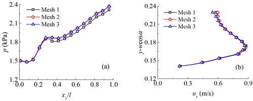
Figure 4. Definition of variables. The flow-velocity profile is cross-sectionally specified, with u_xm as its maximum velocity. l₁ and l₂ are measured vertically and Y and Y₀ in the y direction.

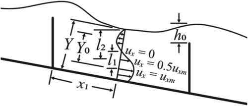
Figure 5(a) compares the water surfaces between the computations and experiments. Simulations 1, 2, and 3 correspond to Tests 1, 2, and 3, respectively. Two types of flow regimes are identified in the tests. At small flow discharges, the water surface over a weir ascends in the flow direction before falling as plunging flow. At large discharges, the water surface becomes approximately parallel to the channel bottom, which also holds true at small pool spacing (skimming flow). These features are well captured in the numerical simulations. The maximum relative errors in the water surface are 7.3, 9.3, and 2.7% in simulations 1, 2 and 3, respectively.

Figure 5. Comparisons between the simulations and experiments by Ead et al. (2004): (a) water depth, (b) velocity profile in plunging regime, and (c) velocity profile in streaming regime.

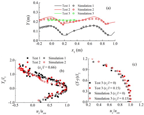
Figure 5(b,c) shows the velocity profile in the plunging and skimming flow regime, where u_xm = maximum cross-sectional value of u_x, l₁ = vertical distance between u_x = u_xm and u_x = 0 points, l₂ = vertical distance between water surface and u_x = 0.5u_xm point, Y₀ = distance between any point and u_x = u_xm point and Y = water depth (Figure 4). Both Y₀ and Y refer to the distances in the y direction (Ead et al. 2004). The velocity data correspond to x₁/l = 0.66 in the plunging flow and x₁/l = 0.15 and 0.30 in the skimming flow. In both regimes, the simulations produce a similar velocity distribution to that in the physical studies. Despite the velocity fluctuations in the plunging flow, the computations are in agreement with the measurements. Smaller discrepancy is evident in the less turbulent flows.

4. Results and discussions

With the validation of the numerical model, 3D simulations are made to examine the effects of θ, w, and l. The analyses focus on weir stage-discharge relationship, velocity profile, turbulent kinetic energy and power dissipation, aiming to evaluate the three layouts and make comparisons. A thorough examination of the parameters gives insight into fishway hydraulics and provides reference for future design. In the middle part of the channel in the flow direction, the flow features in each pool are similar. Hence, the discussions are based on the results at the middle weirs.

4.1. Flow field and stage-discharge relationship

At a weir, the local flow field is an indicator of the fishway hydraulic conditions. To examine the influence of the weir layouts, Figure 6 shows the flow patterns on a plane parallel to the bed at y = 0.5w. The notations denote a combination of geometrical and flow cases, e.g. A1-Q30 refers to Case A1 at Q = 30 L/s.

Figure 6. Flow patterns colored by velocity magnitude – the influence of (a) θ, (b) w, and (c) l on distributions of u_x (m/s) at y = 0.5w. The flow direction is from the left to the right.

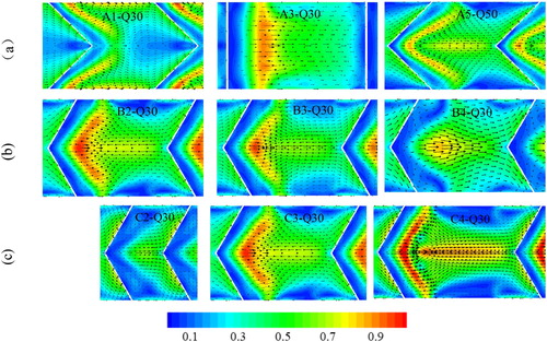
For Layout II, its flow field exhibits a typical two-dimensional pattern without remarkable transverse flow motions; no evident vortex is found downstream. With the nonlinear weirs, unique overflow patterns are produced, which leads to different downstream wakes. In Layout I, for example, the overflow downstream of the weir diverges from the channel center to the sidewalls, while the flow immediately upstream converges to the center from the sides. In Layout III, the flow pattern is opposite of that in Layout I, with the flow, from up- to downstream, first directed to the center and then the walls. In addition, in Layout I, the low velocity regions are along the channel center, while in Layout III they appear along the sidewalls. In Layout II, the high velocity areas cover almost the channel width.

In Layout III, flow circulation along the sidewalls is also observed, which imposes negative impacts on the fish migration efficiency (Marriner et al., 2016). Thus, in this regard, Layouts I and III are suitable for fish species preferring to swim along the sides and center, respectively. In layout III, erosion along the sidewalls might be an issue if placed in a natural channel. With an increase in w, the extent of the high velocity region tends to shrink. However, with an increase in l, it shows an enlargement.

As a function of water stage, the discharge over a straight weir is expressed as (6) $\begin{array}{r}Q=C_d\frac{2}{3}(2g{)}^{1/2}B{h}_0^{3/2}\end{array}$(6) where C_d = discharge coefficient and h₀ = water head above the weir crest (Figure 4). h₀ is calculated by subtracting the weir crest elevation from the maximum water elevation (Kupferschmidt and Zhu, 2017). A V-shaped weir increases the discharge capacity by folding the crest in plan view. The weir crest length b₀ has an effect on the discharge. Therefore, the influence of b₀ needs to be taken into account in discharge prediction. Herein, the parameter B in Eq. (6(6) $\begin{array}{r}Q=C_d\frac{2}{3}(2g{)}^{1/2}B{h}_0^{3/2}\end{array}$(6) ) is replaced by b₀. It is given by (7) $\begin{array}{r}{b}_0=\left\{\begin{array}{l}\frac{B}{\sin \theta }\text{ if }\theta \le {90}^{\circ }\\ \frac{B}{\cos \left(\theta -{90}^{\circ }\right)}\text{ if }\theta >{90}^{\circ }\end{array}\right.\end{array}$(7) The discharge per unit crest length q₀ (= Q/b₀) is introduced (8) $\begin{array}{r}{q}_0=C_0\frac{2}{3}(2g{)}^{1/2}{h}_0^{3/2}\end{array}$(8) where C₀ = discharge coefficient based on b₀. Studies, inclusive of Kupferschmidt and Zhu (2017), show that Q is a function of h₀/n^0.5. Therefore, C₀ is plotted against h₀/n^0.5 (Figure 7), in which some experimental data from a conventional design are also included (Sikora, 1997). With an increase in h₀/n^0.5, C₀ exhibits a decline, with a somewhat larger gradient at the small h₀/n^0.5 values. Based on the simulations, a power-law formula is proposed for the C₀ estimation: (9) $\begin{array}{r}{C}_0=0.487{\left(\frac{h_0}{n^{0.5}}\right)}^{-0.309}\end{array}$(9)

Figure 7. Stage-discharge relationship of V-shaped weirs: (a) C₀ against h₀/n^0.5, and (b) comparison between simulated and predicted C₀ results.

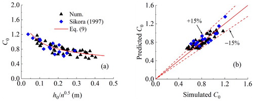
Equation (9) gives a reasonable prediction of C₀, with the coefficient of determination R² = 0.71. Though with some over-estimations, the correlation is consistent with the physical test results by Sikora (1997). The majority of the data sets fall within the relative error band of ±15%. The formula can be used for estimation of stage-discharge relationship of prototype weirs.

4.2. Pool velocity profile

In a pool, the velocity profile is of relevance to the target fish species to rest and migrate upstream. At the mid-point of a pool, Figure 8 presents the u_x/u_xm distribution as a function of Y₀/l₁. The empirical results derived from the conventional pool and weir fishway (Ead et al., 2004) are also included for comparison. (10) $\begin{array}{r}\frac{u_x}{u_{xm}}=\cos \left(\frac{Y_{\text{0}}}{l_1}\right)\end{array}$(10)

Figure 8. Distribution of flow velocity (u_x) at the pool center.

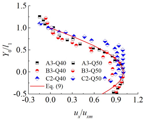
Regardless of weir shape, height and spacing, the dimensionless velocity u_x/u_xm exhibits a cosine-type variation. For Layout II, the flow velocity results are in good agreement with Eq. (10(10) $\begin{array}{r}\frac{u_x}{u_{xm}}=\cos \left(\frac{Y_{\text{0}}}{l_1}\right)\end{array}$(10) ), further confirming the accuracy of the simulations. For either Layout I or III, some discrepancies do exist in between, which is presumably related to the 3D complex flow motions in the V-shaped configurations.

The maximum flow velocity, U_m = (u_x² + u_y² + u_z²)^0.5, is one of the concerns in fishway design. Puertas et al. (2012) suggest that its magnitude should be lower than the burst speed of the target species, which is equal to 10 times the fish body length per second (Hammer 1995). For instance, a common type of salmonid or cyprinid with a body length of 200 mm is believed to migrate upstream favorably if U_m ≤ 2 m/s. To evaluate the efficiency of the V-shaped pool and weir design, an empirical equation is developed for U_m at the symmetry plane. Besides the gravitational acceleration (g), the dominating factors that influence U_m are the channel geometry (n and B), weir arrangement (θ, w and l) and flow discharge (Q): (11) $\begin{array}{r}{U}_m=f_1\left(\theta ,w,l,n,B,Q,g\right)\end{array}$(11) In the light of the principle of homogeneity of dimensions, Eq. (11(11) $\begin{array}{r}{U}_m=f_1\left(\theta ,w,l,n,B,Q,g\right)\end{array}$(11) ) is rewritten as (12) $\begin{array}{r}\frac{U_m^2}{gB}=f_2\left(\frac{{\left(Q{\theta }^n\right)}^2}{g{B}^{7/3}{\left(wl\right)}^{4/3}}\right)\end{array}$(12)

Define geometrical parameter λ = θ²ⁿB^−1/3 (wl)^−4/3 and unit discharge q = Q/B. Then Eq. (12(12) $\begin{array}{r}\frac{U_m^2}{gB}=f_2\left(\frac{{\left(Q{\theta }^n\right)}^2}{g{B}^{7/3}{\left(wl\right)}^{4/3}}\right)\end{array}$(12) ) is transformed into (13) $\begin{array}{r}\frac{U_m^2}{gB}=f_3\left(\frac{\lambda q^2}{g}\right)\end{array}$(13) Figure 9(a) plots the variation of U_m/(gB) against λq²/g. The best-fitted curve takes the power-law form. (14) $\begin{array}{r}\frac{U_m^2}{gB}=0.785{\left(\frac{\lambda q^2}{g}\right)}^{0.366}\end{array}$(14)

Figure 9. Maximum flow velocity (U_m) in the channel: (a) U²_m/(gB) against λq²/g, and (b) comparisons between the simulated and predicted U²_m/(gB).

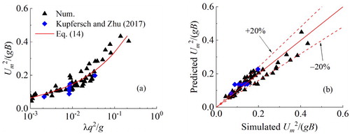
Kupferschmidt and Zhu (2017) conducted experiments in a nature-like fishway with V-shaped boulder weirs. Their data are also included in the analysis to check the accuracy of the proposed relationship. Figure 9(b) shows the comparisons between the simulated and predicted U_m values, with an indication of a ±20% error limit. Both the numerical and experimental results are consistent with Eq. (14(14) $\begin{array}{r}\frac{U_m^2}{gB}=0.785{\left(\frac{\lambda q^2}{g}\right)}^{0.366}\end{array}$(14) ) with R² = 0.89. The proposed formula gives a reasonable prediction of U_m, with most of the data within the ±20% error limit. Moreover, all the U_m values in the studied scenarios are below 2 m/s (the maximum burst swimming speed of a common type of salmonid or cyprinid). Hence, in this regard, these layouts are suitable for the migration of the fish species.

4.3. Turbulent kinetic energy

Turbulent kinetic energy (k) is another parameter of concern, as it takes more energy and longer transit time for target species to migrate along a high k path than a low one (Marriner et al., 2014). The k is defined as (15) $\begin{array}{r}k\text{ = }\frac{1}{2}\left(u_x^{\mathrm{\prime }2}+u_y^{\mathrm{\prime }2}+u_z^{\mathrm{\prime }2}\right)\end{array}$(15) in which u_x′, u_y′, and u_z′ = fluctuating velocities in the x, y, and z directions, respectively. Figure 10 illustrates, at y = 0.5w and Q = 30 L/s, the effects of θ, w and l on k distributions. For Layout I, high k regions are located near the channel walls, while in Layout III they are instead in the channel’s central part. Both layouts present a comparable level of maximum k. In Layout II, the k distribution shows little across-channel changes; its turbulence intensity is lower than that in the V-shaped configurations. This is in agreement with the results from a nature-like fish passage with V-shaped rock weirs (Kupferschmidt and Zhu, 2017).

Figure 10. Turbulent kinetic energy (k, m²/s²) colored by its magnitude – the influence of (a) θ, (b) w, and (c) l at y = 0.5w and Q = 30 L/s.

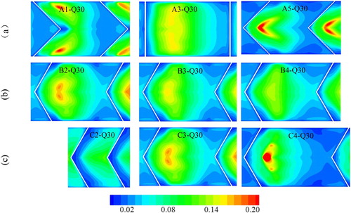
From the perspective of swimming time and energy, the central path in Layout I and the side paths in Layout III are favorable for fish passage. However, its swimming efficiency might be affected by the flow circulations if the fish migrates in the near-wall regions (see section 3.1). Furthermore, to increase w leads to a decline in the magnitude and extent of the high-level k region; to increase l has the opposite effects.

4.4. Pressure distribution

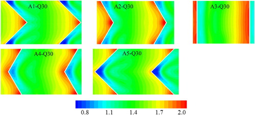
Flow pressure is a proxy of hydraulic loads on the structure. To showcase the effect of the weir geometry, Figure 11 exhibits, for the layouts, the pressure patterns on the channel bottom. In Layout I, the low pressure occurs immediately downstream of the weir near the sidewalls, while the high pressure appears immediately upstream in the center and corners at the walls. In Layout III, the high-pressure zones are similar to those in Layout I, while the low-pressure region is in the channel’s central part. In Layout II, the high pressure distributes uniformly across the channel upstream of the weir. Structural measures might be necessary to enhance the weir stability in the high-pressure areas.

Figure 11. Flow pressure on the channel bottom colored by its magnitude (p, kPa) – contour plots at Q = 30 L/s in Cases A1–A5.

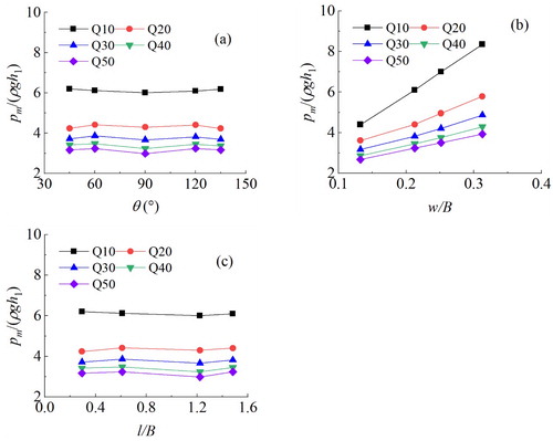
As influenced by the weir parameters, Figure 12 compares the maximum pressure (p_m), in which h₁ = approach flow depth at the channel inlet. A dimensionless pressure variable is defined, p_m/(ρgh₁). The results show that it is insensitive to θ and l; a linear growth is exhibited as w increases. In addition, for a given weir layout, the pressure shows an inverse correlation with Q.

Figure 12. Distribution of flow pressure (p_m) – influence of (a) θ, (b) w, and (c) l on p_m at Q = 10–50 L/s.

4.5. Energy dissipation

To facilitate the target species to pass the pools, a fishway is designed to dissipate the energy of water and maintain a low level of flow velocity (Towler et al., 2015). Therefore, in a single pool, the average energy dissipation rate per unit volume, E, is introduced to evaluate its energy loss, defined as (16) $\begin{array}{r}E=\frac{\rho gQnl}{V_w}\end{array}$(16) in which V_w = water volume in a pool. According to the research by Larinier (2002b), the upper E limits for large salmon and sea trout and for small shad and riverine are 200 and 150 W/m³, respectively. The experimental setup of a rock ramp fish passage in Kupferschmidt and Zhu (2017) are summarized in Table 3. In comparison with the experimental data, Figure 13 plots the E change as a function of q. The results of B2 and C3 are not shown in this figure, as they are the same as A4.

Figure 13. Energy dissipation – variations of E as a function of q.

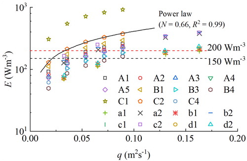
Table 3. Fishway configurations in Kupferschmidt and Zhu (2017).

Test no.	θ (°)	w (cm)	l (cm)	n (%)	Weir material
a1	70	12.5	90	3	Rock
a2				5
b1	120	12.5	90	3	Rock
b2				5
c1	120	12.5	90	3	Concrete
c2				5
d1	70	12.5	90	3	Concrete
d2	90

It is apparent that the simulations (except for C1) and the experiments present a comparable E level. E ascends within an increase in q (as recorded in Yagci 2010). All data yield a similar power-law correlation. The relationship of E and q is described by E = Cq^N, where C = coefficient depending on weir layout, and N = exponent. Despite the difference in weir geometry, the N values in all cases are close to 2/3. For example, C2 data are best fitted with N = 0.66. q is found to be the most influential parameter affecting E, which is presumably related to the energy needed to overcome the gravity.

In case C1, the high E values are likely associated with the small weir spacing (l = ∼0.29B). Therefore, to increase the resting area of target species or lower the E level, enlarging l is a solution, and a short l in a prototype should be avoided. To change w is also effective in the reduction in E. Varying from w = 0.13B to 0.31B, E drops on average by ∼50%. Compared with other factors, θ seems to show the least influence on E. For most of the evaluated scenarios, E is below the 200 W/m³ limit.

5. Conclusions

Hydropower dams affect the river connectivity, forming an obstacle to fish migration and dispersal. A fishway is ecologically necessary to link downstream with upstream. This study introduces an alternative layout with V-shaped (on the plan view) weirs to improve fishway flow conditions. The numerical modeling performed examines the governing factors of weir arm angle, weir height and spacing. The major conclusions are as follows.

• A V-shaped weir produces a diversified velocity field, providing conducive zones for multiple species. For instance, the V-shaped weir with its vertex downstream directs the flow first to the channel walls then to the channel center. As a result, the low-velocity zone is in the channel’s central part. A V-shaped weir with its vertex upstream conveys the water first to the center and then to the walls, with the low-velocity areas along the walls. A conventional design features a 2D flow pattern, with a high-velocity region across the entire channel. A water stage-discharge analysis presents a power law for estimation of the discharge coefficient for the V-shaped layouts.

• A V-shaped weir gives rise to 3D flow motions, with the cross-sectional velocity in the pool showing a cosine-type variation. An empirical formula is proposed for prediction of the maximum velocity over the weir. In the examined cases, its value is below the burst swimming speed of common salmonid and cyprinid.

• For fish migration in a V-shaped layout, the distribution of turbulent kinetic energy (k) indicates that the more favorable path is the channel’s central part if the vertices point downstream and along the sidewalls if the vertices point upstream. Furthermore, increasing the weir height leads to a reduction in both magnitude and extent of the high k region; increasing the weir spacing results in the opposite.

• The maximum pressure is insensitive to either weir angle or spacing. A linear growth is evidenced with an increase in weir height. In addition, for a given weir geometry, the maximum pressure shows a negative correlation with the discharge.

• Energy dissipation is enhanced with an increasing unit discharge. Their relationship is described by a power law with an exponent at approximately 2/3. As the weir spacing or height increases, the energy dissipation exhibits a descending trend. It is however insensitive to the weir angle.

This study deals with a pool-type fishway with V-shaped weirs, and explores its characteristics in terms of flow velocity, turbulence, hydraulic loads and energy loss. In comparison with the conventional design, the primary superiority of the V-shaped layouts lies in the improvement of velocity field and turbulence. A diversified flow field is produced, which is conducive to multiple species. It is an alternative solution to low passage rate fishways. Based on this study, depending on the fish swimming preference, the suggested weir arm angle of the V-shaped design is 60° or 120°. The suitable weir height and spacing are (0.26−0.31) and (1.22−1.48) times channel width, respectively. If the fishway model is implemented to a prototype, the scale is ∼10.

To design a successful fishway, it is a dedicated process. Future work is encouraged to focus on two aspects. One is to examine the hydraulics of fishways, and the other is to study the fish behaviors. Specifically, it is essential to optimize the design by examining additional flow features using both experiments and simulations, such as flow resistance and turbulence intensity. Influencing parameters inclusive of channel slope can be studied. It also requires great efforts from biologists. To improve the design guidance and develop an effective fish passage, documented field observations should also be performed.

Acknowledgements

SVC has been established by the Swedish Energy Agency, Energiforsk and Svenska Kraftnät together with KTH Royal Institute of Technology, Luleå University of Technology, Chalmers University of Technology and Uppsala University. Participating companies and industry associations include AFRY, Andritz Hydro, Boliden, Fortum Generation, Holmen Energi, Jämtkraft, Karlstads Energi, LKAB, Mälarenergi, Norconsult, Rainpower, Skellefteå Kraft, Sollefteåforsens, Statkraft Sverige, Sweco Energuide, Sweco Infrastructure, Tekniska verken i Linköping, Uniper, Vattenfall R&D, Vattenfall Vattenkraft, Voith Hydro, WSP Sverige and Zinkgruvan. The assistance and co-ordinations from Prof. Anders Ansell and Ms. Charlotta Winge of KTH and Ms. Emma Hagner of SVC are acknowledged.

Disclosure statement

No potential conflict of interest was reported by the authors.

Additional information

Funding

The study is part of the research project ‘Two-phase flow modelling: Evaluations and simulations for safer spillway discharge' (VKU14126), funded by the Swedish Hydropower Centre (SVC).

References

- Alvarez-Vázquez, L., Martínez, A., Vázquez-Méndez, M., & Vilar, M. (2008). An optimal shape problem related to the realistic design of river fishways. Ecological Engineering, 32(4), 293–300. https://doi.org/10.1016/j.ecoleng.2007.10.008
- ANSYS Inc. (2019). ANSYS FLUENT Theory Guide. “Release 19.0” ANSYS: Canonsburg, PA, USA.
- Baki, A. B. M., Zhu, D. Z., Harwood, A., Lewis, A., & Healey, K. (2017a). Numerical modelling of rock-weir type nature-like fishpasses, Vancouver, Canada.
- Baki, A. B. M., Zhu, D. Z., Harwood, A., Lewis, A., & Healey, K. (2017b). Rock-weir fishway I: Flow regimes and hydraulic characteristics. Journal of Ecohydraulics, 2(2), 122–141. https://doi.org/10.1080/24705357.2017.1369182
- Baki, A. B. M., Zhu, D. Z., & Rajaratnam, N. (2016). Flow simulation in a rock-ramp fish pass. Journal of Hydraulic Engineering, 142(10), 04016031-1–04016031-12. https://doi.org/10.1061/. doi: 10.1061/(ASCE)HY.1943-7900.0001166
- Bombač, M., Novak, G., Rodič, P., & Četina, M. (2014). Numerical and physical model study of a vertical slot fishway. Journal of Hydrology Hydromechanics, 62(2), 150–159. https://doi.org/10.2478/johh-2014-0013
- Branco, P., Santos, J. M., Katopodis, C., Pinheiro, A., & Ferreira, M. T. (2013). Pool-type fishways: Two different morpho-ecological cyprinid species facing plunging and streaming flows. PloS One, 8(5), 401–424. https://doi.org/10.1371/journal.pone.0065089.
- Caretto, L., Gosman, A., Patankar, S., & Spalding, D. (1973). Two calculation procedures for steady, three-dimensional flows with recirculation, Berlin, Germany.
- Chorda, J., Maubourguet, M. M., Roux, H., Larinier, M., Tarrade, L., & David, L. (2010). Two-dimensional free surface flow numerical model for vertical slot fishways. Journal of Hydraulic Research, 48(2), 141–151. https://doi.org/10.1080/00221681003703956
- Clay, C. H. (2017). Design of fishways and other fish facilities. CRC Press.
- Coşar, A., & Agaccioglu, H. (2004). Discharge coefficient of a triangular side-weir located on a curved channel. Journal of Irrigation and Drainage Engineering, 130(5), 410–423. https://doi.org/10.1061/(ASCE)0733-9437(2004)130:5(410)
- Ead, S., Katopodis, C., Sikora, G., & Rajaratnam, N. (2004). Flow regimes and structure in pool and weir fishways. Journal of Environmental Engineering Science, 3(5), 379–390. https://doi.org/10.1139/s03-073
- Emiroglu, M. E., Kaya, N., & Agaccioglu, H. (2010). Discharge capacity of labyrinth side weir located on a straight channel. Journal of Irrigation and Drainage Engineering, 136(1), 37–46. https://doi.org/10.1061/(ASCE)IR.1943-4774.0000112
- FAO. (2002). Fish passes: design, dimensions, and monitoring.
- Ghalandari, M., Bornassi, S., Shamshirband, S., Mosavi, A., & Chau, K. W. J. E. A. o. C. F. M. (2019). Investigation of submerged structures’ flexibility on sloshing frequency using a boundary element method and finite element analysis. Engineering Applications of Computational Fluid Mechanics, 13(1), 519–528. https://doi.org/10.1080/19942060.2019.1619197
- Ghodsian, M. (2004). Flow over triangular side weir. Scientia Iranica, 11(1), 114–120.
- Hammer, C. (1995). Fatigue and exercise tests with fish. Comparative Biochemistry Physiology Part A: Physiology, 112(1), 1–20. https://doi.org/10.1016/0300-9629(95)00060-K
- Jackson, D. C., & Marmulla, G. (2001). The influence of dams on river fisheries. FAO Fisheries Technical Paper, 419, 1–44.
- Katopodis, C. (1992). Introduction to fishway design. University Crescent.
- Katopodis, C. (2005). Developing a toolkit for fish passage, ecological flow management and fish habitat works. Journal of Hydraulic Research, 43(5), 451–467. https://doi.org/10.1080/00221680509500144
- Katopodis, C. (2015, Jun 28–Jul 03). A review of recent advances in ecohydraulics. 36th IAHR World Congress, the Hague, the Netherlands.
- Katopodis, C., Kells, J., & Acharya, M. (2001). Nature-like and conventional fishways: Alternative concepts? Canadian Water Resources Journal, 26(2), 211–232. https://doi.org/10.4296/cwrj2602211
- Khan, L. A. (2006). A three-dimensional computational fluid dynamics (CFD) model analysis of free surface hydrodynamics and fish passage energetics in a vertical-slot fishway. North American Journal of Fisheries Management, 26(2), 255–267. https://doi.org/10.1577/M05-014.1
- Kim, J. (2001). Hydraulic characteristics by weir type in a pool-weir fishway. Ecological Engineering, 16(3), 425–433. https://doi.org/10.1016/S0925-8574(00)00125-7
- Kisi, O., Emiroglu, M. E., Bilhan, O., & Guven, A. (2012). Prediction of lateral outflow over triangular labyrinth side weirs under subcritical conditions using soft computing approaches. Expert Systems with Applications, 39(3), 3454–3460. https://doi.org/10.1016/j.eswa.2011.09.035
- Kubečka, J., Matěna, J., & Hartvich, P. (1997). Adverse ecological effects of small hydropower stations in the Czech Republic: 1. Bypass plants. Regulated Rivers: Research & Management, 13(2), 101–113. https://doi.org/10.1002/(SICI)1099-1646(199703)13:23.0.CO;2-U. doi: 10.1002/(SICI)1099-1646(199703)13:2<101::AID-RRR439>3.0.CO;2-U
- Kupferschmidt, C., & Zhu, D. (2017). Physical modelling of pool and weir fishways with rock weirs. River Research Applications, 33(7), 1130–1142. https://doi.org/10.1002/rra.3157
- Larinier, M. (2001). Environmental issues, dams and fish migration. FAO Fisheries Technical Paper, 419, 45–89.
- Larinier, M. (2002a). Biological factors to be taken into account in the design of fishways, the concept of obstructions to upstream migration. Bulletin Français De La Peche Et De La Pisciculture, 364(364 supplement), 28–38. https://doi.org/10.1051/kmae/2002105
- Larinier, M. (2002b). Pool fishways, pre-barages and natural bypass channels. Bulletin Français De La Peche Et De La Pisciculture, 364(364 supplement), 54–82. https://doi.org/10.1051/kmae/2002108
- Larinier, M. (2008). Fish passage experience at small-scale hydro-electric power plants in France. Hydrobiologia, 609(1), 97–108. https://doi.org/10.1007/s10750-008-9398-9
- Li, Y., Wang, X., Xuan, G., & Liang, D. (2020). Effect of parameters of pool geometry on flow characteristics in low slope vertical slot fishways. Journal of Hydraulic Research, 58(3), 395–407. https://doi.org/10.1080/00221686.2019.1581666.
- Marriner, B. A., Baki, A. B., Zhu, D. Z., Cooke, S. J., & Katopodis, C. (2016). The hydraulics of a vertical slot fishway: A case study on the multi-species Vianney-Legendre fishway in Quebec, Canada. Ecological Engineering, 90, 190–202. https://doi.org/10.1016/j.ecoleng.2016.01.032
- Marriner, B. A., Baki, A. B. M., Zhu, D. Z., Thiem, J. D., Cooke, S. J., & Katopodis, C. (2014). Field and numerical assessment of turning pool hydraulics in a vertical slot fishway. Ecological Engineering, 63, 88–101. https://doi.org/10.1016/j.ecoleng.2013.12.010
- Mosavi, A., Shamshirband, S., Salwana, E., Chau, K.-w., & Tah, J. H. J. E. A. o. C. F. M. (2019). Prediction of multi-inputs bubble column reactor using a novel hybrid model of computational fluid dynamics and machine learning. Engineering Applications of Computational Fluid Mechanics, 13(1), 482–492. https://doi.org/10.1080/19942060.2019.1613448
- Naghavi, B., Esmaili, K., Yazdi, J., & Vahid, F. K. (2011). An experimental and numerical study on hydraulic characteristics and theoretical equations of circular weirs. Canadian Journal of Civil Engineering, 38(12), 1327–1334. https://doi.org/10.1139/l11-092.
- Nilsson, C., Reidy, C. A., Dynesius, M., & Revenga, C. (2005). Fragmentation and flow regulation of the world's large river systems. Science, 308(5720), 405–408. https://doi.org/10.1126/science.1107887
- Pan, Q., Lu, H., Li, D., & Wang, K. (2017). A new nonlinear iterative method for SPN theory. Annals of Nuclear Energy, 110, 920–927. https://doi.org/10.1016/j.anucene.2017.07.030
- Pan, Q., & Wang, K. (2020). Acceleration method of fission source convergence based on RMC code. Nuclear Engineering and Technology, 52(7), 1347–1354. https://doi.org/10.1016/j.net.2019.12.007
- Puertas, J., Cea, L., Bermúdez, M., Pena, L., Rodríguez, Á, Rabuñal, J. R., Balairón, L., Lara, Á, & Aramburu, E. (2012). Computer application for the analysis and design of vertical slot fishways in accordance with the requirements of the target species. Ecological Engineering, 48, 51–60. https://doi.org/10.1016/j.ecoleng.2011.05.009
- Rajaratnam, N., Katopodis, C., & Mainali, A. (1989). Pool-orifice and pool-orifice-weir fishways. Canadian Journal of Civil Engineering, 16(5), 774–777. https://doi.org/10.1139/l89-112
- Salih, S. Q., Aldlemy, M. S., Rasani, M. R., Ariffin, A., Ya, T. M. Y. S. T., Al-Ansari, N., Yaseen, Z. M., & Chau, K.-W. J. E. A. o. C. F. M. (2019). Thin and sharp edges bodies-fluid interaction simulation using cut-cell immersed boundary method. Engineering Applications of Computational Fluid Mechanics, 13(1), 860–877. https://doi.org/10.1080/19942060.2019.1652209
- Santos, J. M., Silva, A., Katopodis, C., Pinheiro, P., Pinheiro, A., Bochechas, J., & Ferreira, M. T. (2012). Ecohydraulics of pool-type fishways: Getting past the barriers. Ecological Engineering, 48, 38–50. https://doi.org/10.1016/j.ecoleng.2011.03.006
- Sikora, G. J. (1997). An experimental study of flow regimes in pool and weir fishways. University of Alberta.
- Towler, B., Mulligan, K., & Haro, A. (2015). Derivation and application of the energy dissipation factor in the design of fishways. Ecological Engineering, 83, 208–217. https://doi.org/10.1016/j.ecoleng.2015.06.014
- Wang, R. W., David, L., & Larinier, M. (2010). Contribution of experimental fluid mechanics to the design of vertical slot fish passes. Knowledge Management of Aquatic Ecosystems, 396(2), 1–21. https://doi.org/10.1051/kmae/2010002.
- Xu, T., & Jin, Y.-C. (2014). Numerical investigation of flow in pool-and-weir fishways using a meshless particle method. Journal of Hydraulic Research, 52(6), 849–861. https://doi.org/10.1080/00221686.2014.948501
- Yagci, O. (2010). Hydraulic aspects of pool-weir fishways as ecologically friendly water structure. Ecological Engineering, 36(1), 36–46. https://doi.org/10.1016/j.ecoleng.2009.09.007