Experimental and numerical research on wind characteristics affected by actual mountain ridges and windbreaks: a case study of the Lanzhou-Xinjiang high-speed railway

Abstract

To reduce the impact of a mountain ridge on the crosswind flow field of a specific section of the Lanzhou-Xinjiang high-speed railway, a portion of the mountain ridge was removed to increase the distance from the windbreak. To verify the effects of this flow optimization measure, the wind speed and wind angle were tested in this mountain ridge region. In this paper, under the actual conditions of this specific case study, the average and transient wind characteristics were analyzed based on the test results. Then, based on the actual terrain model, using the computational fluid dynamics (CFD) method with two inlet boundary conditions, namely, constant wind and exponential wind, the results obtained from the two boundary conditions were validated. Furthermore, the visualized flow structures and wind speed distributions along the railway under both boundary conditions were compared. Finally, along the railway, the impacts of different terrain types on the flow field of the railway were compared.

KEYWORDS:

• Mountain ridges
• windbreak
• terrain
• crosswind
• experiment
• CFD

1. Introduction

The effects of crosswind on traffic and transportation are severe worldwide, and many accidents, including road and railway vehicle accidents, occur due to the impact of crosswind conditions every year (Baker et al., 2009). Therefore, studies on train aerodynamics under crosswind conditions have been conducted (Baker et al., 2004; Chen et al., 2018; Liu et al., 2018; Zhang et al., 2018). To study the aerodynamic performance of a train under crosswind conditions and to obtain the characteristic wind curves (CWCs) at different train speeds, Cheli et al. (2010) conducted a wind tunnel experiment and numerical simulations on the new EMUV250 train under crosswind conditions in Italy, and three versions of the train were considered in terms of the force and moment aerodynamic coefficients.

Generally, in addition to the train itself (Chen et al., 2019; Hemida & Krajnović, 2008; Li et al., 2018; Niu et al., 2017; Zhang et al., 2011), different railway line types also influence the trains under crosswind conditions. Trains regularly may pass by flat ground, embankments, cuttings, and bridges (Zhang et al., 2015). Trains face more significant overturning risks at higher positions under strong winds. Therefore, when traveling over embankments and bridges, trains are more dangerous (Gao & Miao, 2010; Noguchi et al., 2019; Tomasini et al., 2014; Wang et al., 2018). However, sometimes the railway lines pass through constantly changing terrain types, which generates connection and transition regions between two terrain types, such as the transition regions between a cutting and an embankment or a tunnel and a bridge. This transition region provides an additional sudden wind load on the train under crosswinds, and the train aerodynamic performance and dynamic index change suddenly (Li et al., 2012, 2019; Wu et al., 2015, 2017; Yang et al., 2018; Zhang, Zhang, et al., 2019).

To reduce the influence of strong crosswinds, wind barriers are commonly built because of their low costs and high effectiveness. Similarly, windbreak types and their effectiveness on bridges (Guo et al., 2015; He et al., 2019; Zhang, Gao, et al., 2013; Zhang, Xia, et al., 2013), embankments (Avila-Sanchez et al., 2010, 2014; Gao & Duan, 2011) and flat ground (Hashmi et al., 2019; Yang et al., 2011; Zhang et al., 2017; Zhang, He, et al., 2019) have been studied to protect trains. In addition, due to the effects of the terrain, wind-reducing facilities are discontinuous and sometimes generate transition areas between different landforms, such as the windbreak transition induced by a regular windbreak and an open-hole tunnel or between a cutting and an embankment, bridge, or a tunnel (Deng et al., 2019; Sun et al., 2019, 2020; Wang, 2010). In this windbreak transition region, due to the sudden structural shape change, the original wind-reducing ability is weakened, and there is a strong wind impact on the train (Chen et al., 2019; Liu et al., 2018; Xu et al., 2019).

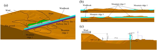
In addition to windbreak transitions, in practice, the presence of tall structures and facilities in positions close to the windbreak can also cause a sudden drop in the protection ability of the windbreak. For example, the Lanzhou-Xinjiang high-speed railway in China passes through a strong wind area, and windbreaks have been built along parts of the railway. Some locations are mountainous, so cuttings have been dug. However, in some areas, only a mountain ridge is beside the railway, and the length of the mountain ridge along the railway is not sufficient to make a cutting. To maintain a regular shape, windbreaks are built close to the mountain ridge. Generally, the protective effect of 4-m-high windbreaks is very good. However, in full-scale tests under strong winds, it was found that in some flat ground or embankment regions with 4-m-high windbreaks, the wind load exhibited a sudden increase (Chen et al., 2016; Liu, Chen, et al., 2015; Liu, Su, et al., 2015; Lu et al., 2014). To determine the cause of this problem, an on-site inspection was organized in areas where the wind load changed suddenly. Finally, it was found that the heights of some mountain ridges were equal and even higher than the height of the windbreak, and if the mountain ridge was very close to the windbreak, it failed to provide a wind-reducing ability in the local area. Therefore, for a flow optimization measures, a part of the mountain ridge was removed, and a flat ground region was generated between the windbreak and the mountain ridge, as shown in Figure 1. To validate the effectiveness of such measures, an experiment was conducted to test the wind speed and wind angle outside and inside the railway.

Figure 1. The landform of the measurement site beside the high-speed railway: (a) the entire view; (b) the WWS view and LWS view; and (c) the size from the front view.

This paper differs from previous studies, which focused on simplified or ideal models and have rarely studied the effects of a mountain ridge with complex terrain on windbreaks. In the present work, the experimental results were first analyzed, and the basic wind speed and wind angle distribution around the railway were obtained. The test results showed the reliability of the present flow optimization measure: a part of the mountain ridge was removed to increase the distance from the windbreak. Then, with the help of the computational fluid dynamics (CFD) analysis, which provides accurate predictions for engineering research (Ghalandari et al., 2019; Mou et al., 2017; Salih et al., 2019), numerical simulations were performed based on the actual terrain. The visualized flow field structure was analyzed in detail. In particular, unlike in previous studies mentioned before, two inlet boundary conditions – constant wind and exponential wind – were compared. Furthermore, in addition to the experimental region, the impacts of different terrains on the flow field of the railway were also compared in detail.

2. Experimental description

2.1. Measurement site and the layout of the test points

The landform model of the measurement site is shown in Figure 1. On the windward side (WWS), two mountain ridges exist outside the windbreak. Between the mountain ridges and the windbreak, flat ground with a width of 25 m exists to reduce the direct impact of airflow from the mountain ridges. The tops of the mountain ridges and the flat area are connected by the slope depicted in green in Figure 1(a). The figure shows that the height of mountain ridge 2 is 5.4 m, which is higher than the height of the windbreak, and the slope angle is $\text{ tan}\theta =1:1.5$.

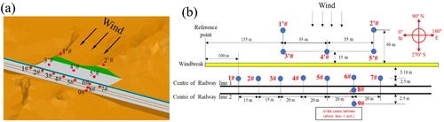
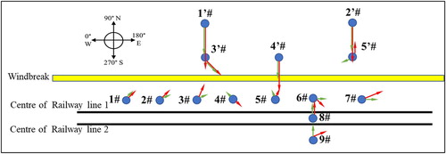
Figure 2 shows the relative positions of the different test points; Figure 2(a) presents a 3D view, and Figure 2(b) shows a top view and the detailed distances between different test points. Five test points are located outside the windbreak, and test points 1’# and 2’# are located on the tops of mountain ridges 1 and 2, respectively; the points are set as references for remote wind speed. Test points 3’#, 4’# and 5’# are set on the flat land between the mountain and the windbreak, and test point 4’# is located between test points 3’# and 5’#. Nine test points are located along the railway, and test points 1#-7# are located along a straight line between the windbreak and the center of railway line 1. Test point 8# is at the center of the two railway lines, and test point 9# is on the leeward side (LWS) of railway line 2 at a distance of 2.5 m from the center of railway line 2.

Figure 2. The layout of the test points: (a) the entire view and (b) the distances between different test points.

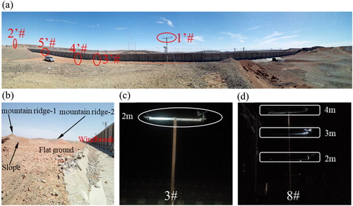
The experiment was conducted during the train outage time from 0:00 to 4:00 in the early morning, and the test points outside the windbreak were arranged during the daytime. However, the test points on the railway were arranged, tested and removed from the railway before 4:00 in the morning. Therefore, the test points outside the railway are clearly visible in Figure 3(a), and the test points on the railway are dark, as shown in Figure 3(c,d). Moreover, the actual landscape outside the windbreak is shown in Figure 3(b). A pair of wind angle and wind speed sensors are located on top of every wind measurement rod outside the railway, and the sensors are 4 m from the ground, as shown in Figure 3(a). On the railway, a pair of wind angle and wind speed sensors are located on top of every wind measurement rod for test points 1#-7#, and the sensors are all 2 m above the top of the rail (TOR), as shown in Figure 3(c). For test points 8# and 9#, three pairs of wind direction and wind speed sensors are located on top of the wind measurement rods, as shown in Figure 3(d).

Figure 3. The test points in the real site: (a) outside the windbreak; (b) the landform; and (c) test points 3# and (d) 8# on the railway.

2.2. The measurement device and data processing

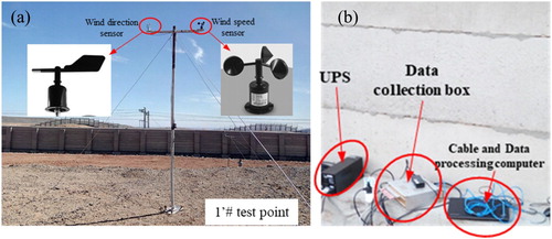
The wind speeds and angles were determined by three-cup anemometer sensors, as shown in Figure 4(a). The measurement ranges of the sensors are 0–70 m/s and 0–360°, the measurement accuracies are ±2% and ±2°, and the working conditions are between −40°C and 50°C and 5–95% relative humidity (RH), respectively. Additionally, the starting wind speed is $\le$0.5 m/s. The data collection and processing system is shown in Figure 4(b); the system includes an uninterruptible power system (UPS), data signal lines, a data collection box, a cable and a data processing computer. The data are collected at 60 Hz, and the data collection box has the advantage of simultaneous multichannel data acquisition. The wind speed data outside and inside the windbreak were collected at the same time.

Figure 4. Measurement devices: (a) wind speed and direction sensors and (b) the data collection and processing system.

3. Analysis of the test results

3.1. Average wind characteristics

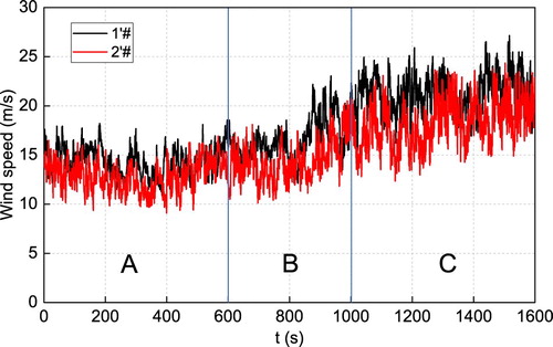
Figure 5 shows the remote wind speed at test points 1’# and 2’# outside the windbreak. The test duration for wind speed and angle measurements outside and on the railway was approximately 1600 s. In Region A, during t = 0–600 s (10 min), the upcoming flow speed is low. In Region B, the wind speed increases gradually. In Region C, during t = 1000–1600 s (10 min), the wind speed remains at a higher level. Therefore, the present work focuses on the two stages in Region A and Region C to thoroughly analyse the wind characteristics.

Figure 5. The wind speeds at test points 1’# and 2’# are remote reference wind speeds.

The wind speed curves outside the windbreak and on the railway in the low wind speed stage are shown in Figure 6. The wind speeds are highest at test points 1’# and 2’#, which feature similar speeds. For test point 4’#, which is affected by the acceleration effect of the concave ground between mountain ridges 1 and 2, the value is relatively higher than that at 3’# because the height of mountain ridge 1 is lower than that of mountain ridge 2, and the greater shelter effect of mountain ridge 2 results in the lowest value for test point 5’#.

Figure 6. The wind speeds at the test points in the low wind speed stage: (a) 1’#-5’# outside the windbreak and (b) 1#-7# and (c) 8#-9# on the railway.

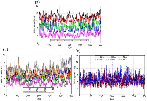
On the railway, due to the effect of the windbreak, the wind speeds at test points 1#-7# are low, with values of approximately 2–10 m/s. Test points 8# and 9# are relatively far from the windbreak, and their wind speeds are therefore higher than those at test points 1#-7#. Furthermore, for test points 8# and 9#, the wind speed at the higher position is higher than that at the lower position. In addition, because the distance from test point 9# to the windbreak is the longest, the wind speed at each height is higher than that at test point 8#. In the high wind speed stage, the relationships and patterns between each test point are similar and are not discussed further.

As an intuitive representation of wind speeds and angles, Figure 7 shows rose diagrams of test points 1’#-5’# outside the windbreak and test points 1#, 3#, 5#, 7# and 9#-3 m on the railway in the low and high wind speed stages. In the low wind speed stage depicted in Figure 7(a), the primary wind angle of the remote wind on mountain ridges 1 and 2 is 90°. For test point 3’#, which is affected by the partial shelter effect of mountain ridge 1 and the other flows originating from the gap between mountain ridge 1 and the windbreak, the major wind angle is 45°. Additionally, the major wind angle at test point 4’# is similar to those at test points 1’# and 2’# because test point 4’# is located in the concave area between the two mountain ridges with a weak shelter effect. Test point 5’# is fully sheltered by the higher mountain ridge 2, and the corresponding wind angle is disorderly. On the railway, the phenomenon of reverse reflow is distinct at test point 9#-3 m, which is farther from the windbreak than test points 1#-7#, resulting in a major wind direction of 270°. For the test points near the windbreak, reverse reflow is stopped and compressed by the windbreak; therefore, the wind angles at these test points are variable, exhibiting trends that follow the longitudinal direction of the railway line, resulting in wind angles mainly in the range of 270–360° at these test points.

Figure 7. Rose diagrams of wind speeds and directions: (a) the low wind speed stage in Region A and (b) the high wind speed stage in Region C.

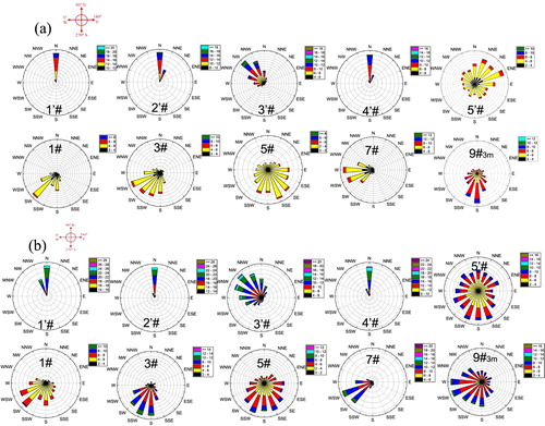
In the high wind speed stage depicted in Figure 7(b), overall, the major wind directions at all test points are slightly different from those in the low wind speed stage, but the distribution range of the wind direction becomes wider. Outside the windbreak, the major wind directions of the remote wind at test points 1’# and 2’# are also approximately 90°, but the test points have trends of less than 90°. Test point 4’# also shows the same trend. Furthermore, the wind direction ranges at test points 3’# and 5’# are 0–90° and almost 0–360°, respectively.

The primary wind angles and the average 10-min wind speeds in the low and high wind speed stages are shown in Figure 8. The green arrow denotes the low wind speed stage, and the red arrow denotes the high wind speed stage. Note that the values at test points 8# and 9# correspond to the middle height of 3 m. The length represents the wind speed. Here, the average 10-min wind speeds at test points 1’# and 2’# in the high wind speed stage are 21.34 and 18.25 m/s, respectively.

Figure 8. The wind speed and direction distributions at the different test points in the low and high wind speed stages.

In addition, Table 1 shows the dimensionless wind speed coefficient $U$ for the different test points on the railway considering the average 10-min wind speed in the low and high wind speed stages. $U$ is defined in Equation (1)(1) $\begin{array}{r}U=\frac{U_{\text{railway}}}{U_{\text{inlet}}}\end{array}$(1) . Here, $U_{\text{inlet}}$ is selected at test point 1’#. The total wind speed value, $U$, in the low and high wind speed stages is in the range of 0.2–0.5 for the test points (1#-7#) located between the windbreak and railway line 1; $U$ is in the range of 0.3–0.5 for the test points (8# and 9#) located on the railway line. However, for the wind speed perpendicular to the railway, which has a significant impact on trains, $U$ is lower and in the range of 0–0.3 for test points 1#-7# in the low and high wind speed stages. For the test points located on the railway lines, certain differences exist in the low and high wind speed stages; namely, $U$ is in the range of 0.3–0.45 in the low wind speed stage but in the range of 0–0.35 in the high wind speed stage. The value of $U$ in the high wind speed stage is substantially lower, but the fluctuation range is wider. Overall, the current results show that the current flow optimization measure is effective in reducing the wind speed over the railway. (1) $\begin{array}{r}U=\frac{U_{\text{railway}}}{U_{\text{inlet}}}\end{array}$(1)

Table 1. The dimensionless wind speed coefficient $U$ for every test point on the railway.

		1#	2#	3#	4#	5#	6#	7#	8#-2 m	8#-3 m	8#-4 m	9#-2 m	9#-3 m	9#-4m
Total wind speed	low	0.31	0.32	0.32	0.24	0.2	0.36	0.44	0.43	0.41	0.46	0.45	0.45	0.47
	high	0.25	0.27	0.34	0.2	0.2	0.26	0.47	0.34	0.33	0.36	0.35	0.34	0.36
Lateral wind speed	low	0.22	0.12	0.12	0.17	0.18	0	0	0.43	0.41	0.33	0.42	0.45	0.43
	high	0.18	0.19	0.31	0.14	0.18	0.18	0.18	0.31	0.13	0	0.32	0.13	0.14

3.2. Fluctuating wind characteristics

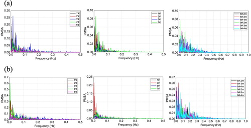
Figure 9 shows the fluctuation frequency of wind speed at test points 1’#-5’# outside the windbreak and at test points 1#, 3#, 5#, 7#, 8# and 9# on the railway in the low and high wind speed stages, respectively. The y-axis is the power as the mean squared amplitude (PMSA). In the low wind speed stage, the domain frequencies (DFs) of test points 1’#-5’# are mainly in the range of 0–0.2 Hz. On the railway, the DF range is 0–0.25 Hz for test points 1#-7#, but is 0–0.46 Hz for test points 8# and 9#, which are relatively farther from the windbreak. In the high wind speed stage, with increasing wind speed, the corresponding DFs for test points 1’#-5’#, 1#-7# and 8#-9# are 0–0.3, 0–0.3, and 0–0.5 Hz, respectively. Overall, the ranges of the DFs for the different test points slightly increase as the wind speed increases.

Figure 9. The PMSA of the different test points: (a) the low wind speed stage in Region A and (b) the high wind speed stage in Region C.

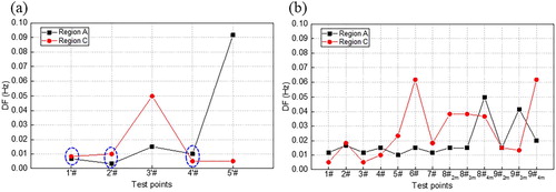
Furthermore, the first DFs corresponding to the maximum PMSAs at the different test points are shown in Figure 10. Outside the windbreak, the first DFs in the low wind speed and high wind speed stages change slightly for test points 1’#, 2’# and 4’#, and the results from these points represent the remote upcoming flow without any obstruction to a certain extent. Affected by the shelter provided by the slope, the first DFs for test points 3’# and 5’# differ substantially at different wind speeds. In terms of the first DFs on the railway, which is affected by the windbreak, in the low wind speed stage, the first DFs for test points 1#-7#, 8#-2 m, 8#-3 m, 9#-2 m and 9#-4 m are close to each other, with ranges of 0.01–0.02 Hz. In the high wind speed stage, the first DFs of the different test points show no clear patterns, but overall, a higher wind speed seems to result in a higher first DF for most test points.

Figure 10. The first DFs of the different test points: (a) outside the windbreak and (b) on the railway.

Turbulence intensity I represents the intensity of wind velocity fluctuation in time and space. I is defined in Equation (2) as the ratio of the standard deviation $\sigma$ of the fluctuating wind velocity to the mean 10-min wind speed $\overline{U}$. In addition, the gust factor G represents wind fluctuation during a certain time. G is defined in Equation (3), where $U_{tg}$ is the maximum wind speed during a certain time $tg$, and generally, $tg=3s$. According to the definition, Figure 11 shows the I and G values at the different test points in the low and high wind speed stages.

Figure 11. The turbulence intensity I and the gust factor G at different wind speeds: (a) outside the windbreak and (b) on the railway.

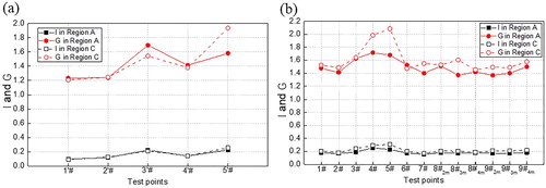
Outside the windbreak, the I values at test points 1’#-5’# show almost no change as the wind speed increases and are in the range of 0.1–0.3. The range of G is larger than that of I at 1.2–2.0 in the low and high wind speed stages. Moreover, the G values at test points 1’#, 2’# and 4’# also show no notable change as the wind speed increases, but the G values at test points 3’# and 5’# clearly change. On the railway, in the low and high wind speed stages, the ranges of I and G are 0.1–0.4 and 1.3–2.1, respectively. Overall, I and G increase from test points 1# to 5# and then decrease until test point 6#, and the I and G values of each test point are similar at test points 6# to 9#. However, the I and G values in the high wind speed stage are higher than those in the low wind speed stage for each test point. (2) $\begin{array}{rl}I& =\frac{\sigma }{\overline{U}}\end{array}$(2) (3) $\begin{array}{rl}G& =\frac{U_{tg}}{\overline{U}}\end{array}$(3)

4. CFD analysis of the terrain around the railway

Based on the analysis of test results in Section 3, the primary wind field information, including the average wind speeds and wind angles, and fluctuation wind characteristics outside and inside the railway were obtained. Furthermore, it shows that under the current flow optimization measure, namely, an area of flat ground 25 m wide from the mountain ridge to the windbreak, the wind speed coefficient $U$ perpendicular to the railway lines is less than 0.45 (9 m/s). Therefore, this measure is useful in the mountain ridge region. However, the flow mechanism around the mountain ridge region and the impact of neighboring terrains on the railway remain unclear. Thus, in the following sections, based on the actual terrain model discussed in Section 3, CFD technology is used to study the detailed flow structures induced by the different terrains around the railway.

4.1. The computation method and the computational domain

To better satisfy the requirement of the mesh size of the numerical method, a 1/10-scale model was used in the computation. The unsteady Reynolds-averaged Navier–Stokes (URANS) equation is used in most numerical studies involving these conditions to describe the time-averaged flow; the results obtained by this equation are also valid for determining the pressure field, velocity field, and aerodynamic forces (Haque et al., 2016; Liu et al., 2018). According to a previous study conducted by Morden et al. (2015), the shear stress transport (SST) $k-\omega$ approach can reduce the computational expense with a slight reduction in accuracy when predicting forces and surface pressures. Therefore, the three-dimensional incompressible URANS equations and the $\text{SST}k-\omega$ turbulence model (Menter, 1994) are used in this paper. The commercial software package Fluent is used, and the governing equations are discretized by the finite volume method (FVM). The convection and diffusion terms are discretized by the second-order upwind scheme, and the time derivative is discretized by the second-order implicit scheme for unsteady flow calculations. The time-step, $\mathrm{\Delta }t,$ is $1\times {10}^{-4}\text{s}$. The velocity-pressure coupling and solution procedures are based on the semi-implicit method for pressure-linked equations consistent (SIMPLEC) algorithm (Van Doormaal & Raithby, 1984).

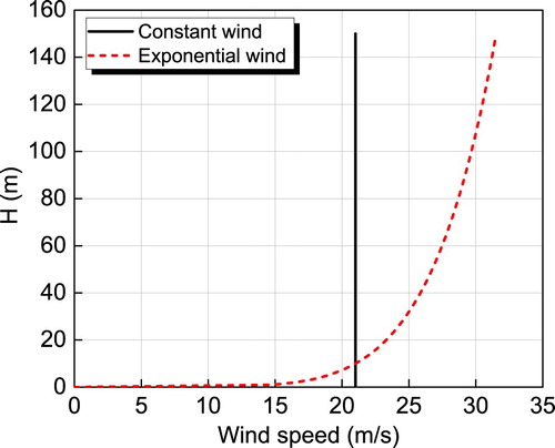
Figure 12 shows the computational domain and the corresponding boundary conditions for simulating the flow field in the high wind speed stage discussed before. For a more intuitive understanding, here, the dimension is shown by the full-scale size. The dashed rectangle is the landform where the test was conducted. Face BFGC is set as the velocity inlet and refers to the average wind speed of test point 1’#, which is 21.34 m/s, and the wind angle is 90°. Meanwhile, as shown in Figure 13, two inlet boundary conditions are simulated: constant wind and exponential wind along the height. For the exponential wind, the velocity inlet is set as $u={\left(\frac{z}{z_{10}}\right)}^{\alpha }{u}_{10}$, where $u$ is the wind speed at a height of $z$ and $u_{10}$ is the standard wind speed (the wind speed at the reference height $z_{10}$). In China, the wind speed at a height of 10 m is defined as the standard wind speed (Huang & Wang, 2008), and the measuring point at the top of the mountain is also approximately 10 m from the ground. Thus, $z_{10}$ = 10 m and $u_{10}$ = 21.34 m/s are used in this paper. $\alpha$ is the ground roughness factor; here, $\alpha$ = 0.15. Faces ABCD and EFGH and top surface DCGH are all set symmetry conditions. Face AEHD is set as a zero-pressure outlet condition. The ground and the windbreak are set as no-slip wall conditions.

Figure 12. The computational domain and boundary conditions.

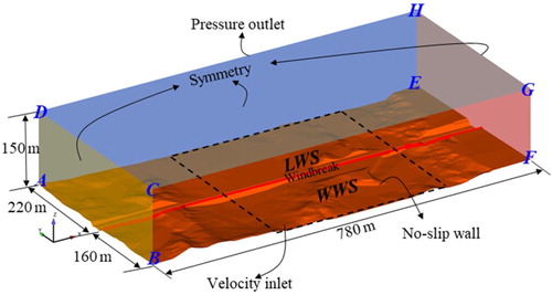
Figure 13. The inlet boundary conditions used in this study.

4.2. Mesh strategy and result validation

Figure 14 shows the computational mesh. Four different refinement areas exist from the WWS to the LWS. To analyse the flow field around the railway, the area of part B is the most important and consists of the areas on both sides of the railway and windbreak. The width is 100 m, and the grid size is small. Furthermore, the flow field information on the LWS is more important than that on the WWS, and the mesh size in part C is therefore slightly larger than that in part B, with a width of 50 m. The last areas, including the upstream area in part A and the downstream area in part D, have the same mesh size, which is slightly larger than that in part C. In the space shown in Figure 14(b), two boxes have been added to refine the mesh, and Figure 14(c) shows the mesh around the windbreak. To ensure that the velocity gradients near the wall are correct, ten prism layers of cells are applied to the surface of the model, the extension ratio of each cell is 1, and the thickness of the first prism layer is 0.3 mm, resulting in an average$y^{+}$ around the model of less than 20. According to the ANSYS Fluent Theory Guide (Fluent, 2013), the $\omega$-equation can be integrated through the viscous sublayer by using a $y^{+}$-insensitive wall treatment, which blends the viscous sublayer formulation and the logarithmic layer formulation based on $y^{+}$. This formulation is the default method for all $\omega$-equation-based models. An enhanced wall treatment (EWT) is used in this paper to determine the shear stress at the first cell close to the wall. Therefore, the calculations in this paper are feasible. The total number of volume meshes is more than 41 million.

Figure 14. The computational mesh.

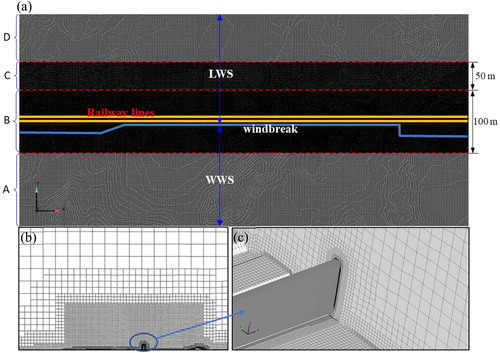
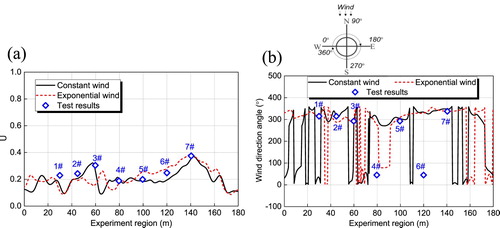
Figure 15 shows the average result comparison of wind speed and wind angles between the simulation and the test results. Overall, for both inlet boundary conditions, the trends of the simulation results for wind speed and wind angles are approximately in agreement with the full-scale test results. However, there are slight position differences between the numerical simulation results and the experimental results. Ignoring these slight position differences, and in terms of the results in similar positions from the simulation and the experiments, the maximum error of constant wind is no larger than 7%, and the maximum error of exponential wind is no larger than 10%. Note that because the wind speed coefficient is relatively small and the wind direction changes by approximately 0° (360°), the relative error may be larger. In this mountain ridge region, with the flat ground between the windbreak and the mountain ridges, the exponential wind boundary does not show absolute advantages over the constant wind speed boundary, possibly because the height range around the railway is not very large. Considering the complicated terrains, both simulation results are acceptable in terms of the trends and values.

Figure 15. Comparison of the results between the simulation and the full-scale test: (a) wind speed and (b) wind direction angles.

4.3. Results comparison between different inlet boundary conditions

To further study the differences between both boundary conditions for the test region, as shown in Figure 16, the wind speeds perpendicular to the railway under both boundary conditions are compared. Here, two heights – 2 m (near the middle height of the train) and 4 m (near the top of the train) from the TOR – are selected along railway lines 1 and 2 (RL-1 and RL-2, respectively). As shown in the circle, the difference between the constant wind and exponential wind at the lower position is larger than that at the higher position of 4 m. Furthermore, the trends along the same railway are closer to each other at different heights under exponential wind conditions, which can be observed in the circle.

Figure 16. The wind speed comparison between the constant wind and exponential wind boundary conditions: (a) RL-1; and (b) RL-2.

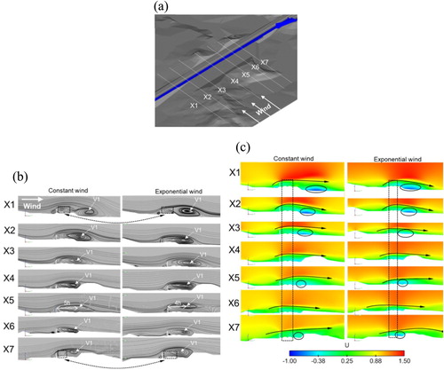
Figure 17(a) shows streamlines at heights of 2 and 4 m for both boundary conditions. At a height of 2 m, differences are apparent in Regions A, C and D, but in Region B, the streamlines are similar for both boundary conditions. At the height of 4 m, the differences are smaller in Regions A and B, and the differences are more significant in Regions C and D. In particular, at the height of 2 m, the vortex in Region A is more stable for the exponential wind; in Region C, some smaller vortices are present in the range of the railway width in the exponential wind case; however, in the constant wind case, a large vortex is present on the LWS of RL-2, which does not occur in the exponential wind case. In Region D, a large steady vortex is present in the inlet of the cutting area in the constant wind case, but only disordered and smaller vortices occur near the windbreak in the exponential wind case. At the height of 4 m, Region A in the constant wind case changes and becomes similar to that in the exponential wind case. However, the differences in Regions C and D are similar to those at the height of 2 m. Although the flow structures of both boundary conditions in some positions are different, the wind speed is not high at the railway due to the effective windbreaks. Therefore, as shown in Figure 17(b), in the width range of the railway, the differences in wind speed distribution in Regions B and C at the height of 2 m and in Regions A-C at the height of 4 m are smaller, which is why the wind speed curve at the height of 4 m in Figure 16 shows similar changes under both boundary conditions. Furthermore, corresponding to the experiment site, most test points are in Region B; here, the streamlines show that in the width range of the railway, the backflow occurs but is blocked by the windbreak. Then, the airflow in the railway has a motion trend along the railway, and this motion trend is the same as the wind angles of the test results. Meanwhile, with a 25 m width from the mountain ridge to the windbreak, the strong wind is effectively blocked by the windbreak. The wind speed coefficient $U$ in the railway is less than 0.45 in Regions B and C, and this wind speed range is also the same as the test results.

Figure 17. The flow field comparison between the constant wind and exponential wind boundary conditions: (a) streamlines and (b) the wind speed distribution contour.

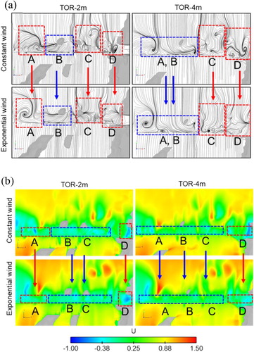
Figure 18 shows the streamlines and corresponding speed distribution contours at different cross-sections along the railway. On the LWS of the windbreak, vortex V1 is generated, and the differences between the constant wind and exponential wind boundary conditions are mainly in cross-sections X1, X5 and X7; these positions are mainly in the edge of the mountain ridges. At X1, a vortex occurs in the railway for the constant wind boundary, but no such vortex emerges for the exponential wind boundary. At X5, the distance from the vortex core of V1 to the windbreak is 5 h for the constant wind boundary but 4 h for the exponential wind boundary; here, h is the train height: 3.7 m. At X7, the airflow above the railway is not a part of vortex V1 for the constant wind boundary, but for the exponential wind boundary, V1 occupies the entire width of the railway. For the corresponding wind speed distribution at X1-X7, the differences in the two boundary conditions are shown in the direction of the arrow and the circle positions, namely, the airflow directions show some differences at X1, X6 and X7, and the speed distributions show some differences on the LWS of RL-2 at most positions. However, as shown in the dashed box, the speed distributions in the range of the railway are similar due to the effective shielding effect of the windbreak.

Figure 18. The flow field comparison between the constant wind and exponential wind boundary conditions in different cross-sections: (a) the positions of different cross-sections; (b) streamlines; and (c) the wind speed distribution contour.

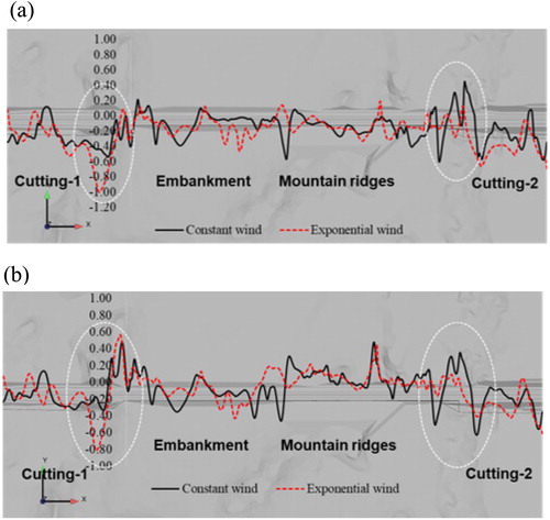
Finally, for an overall comparison, Figure 19 shows the wind speed coefficient $U$ along the railway for RL-2 at different heights from the TOR. A difference always exists between the two boundaries along the railway, but in the embankment and mountain ridge region, the wind speed changes within a small range. Therefore, the differences between the boundary conditions are relatively small. However, as shown in the circle, the differences in the terrain transition regions are obvious and significant, and these differences do not show a consistent pattern at different locations along the railway. Namely, the wind speed obtained from the exponential wind is not absolutely higher or lower than that obtained from the constant wind. However, in the deeper cutting area (shown in the left circle), where the wind-reducing capacity of the windbreak is excessive, the results obtained from the exponential wind are strong, and the distance between peaks of sudden changes in wind speed is larger. However, at the position where the windbreak’s wind-reducing capacity is insufficient (shown in the right circle), the results obtained from the constant wind are larger.

Figure 19. The wind speed comparison along RL-2 between the two boundary conditions: (a) TOR-2 m; and (b) TOR-4 m.

4.4. Comparison of flow structures in different terrains around the railway

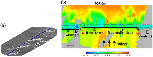
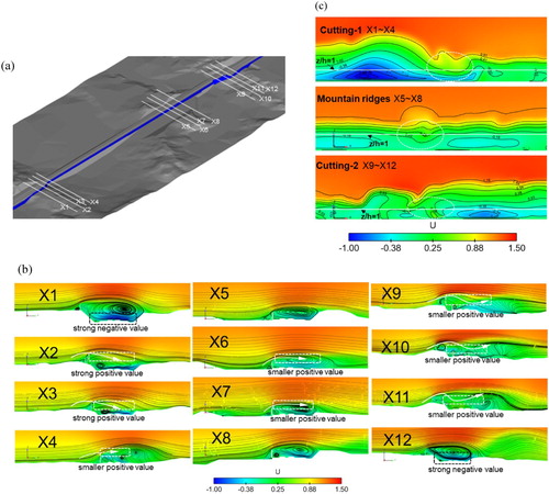
As shown in Figure 20, based on the results under the exponential wind boundary condition, the impacts of different terrains on the flow field of the railway are compared in this section. The entire terrain includes cutting areas (Regions A, B, and E), an embankment (Region C), and mountain ridges (Region D). In cutting Regions A and E, the wind speed is low and negative, but in cutting Region B, the negative wind speed value is higher than in Regions A and E because the cutting area is deeper for Region B. In embankment Region C, the wind speeds at most positions are also low and negative because of the good shielding effect of the windbreak. In mountain Region D, due to the 25-m-wide area of flat ground between the mountain and the windbreak, the wind speed at the railway is not higher. In addition, two positions – Regions F and G – serve as the connecting region between the cutting areas and the embankment. Due to sudden changes in the terrain and the windbreak height and shapes, a sudden change in wind speed occurs, and the quantitative wind speed changes at both positions can be seen in Figure 19.

Figure 20. The wind speed distribution contour at a height of 3 m from the TOR.

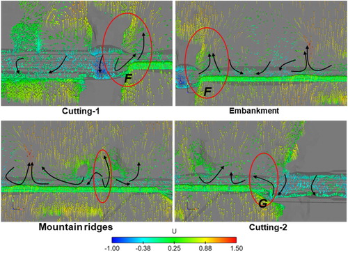
Furthermore, Figure 21 shows the speed vector at a height of 3 m from the TOR. In the cutting areas and embankment, the backflow predominantly exists at the railway and leads to a smaller negative wind speed. At the railway in the mountain ridge area, the narrow space between the LWS mountain and the windbreak causes the airflow to run along the railway, which again validates the test results. Additionally, note that in the red circle in the mountain ridge region, sudden air release occurs between the two mountain ridges on the LWS of RL-2, leading to a slight positive wind speed in the railway. Additionally, for the windbreak transition, as shown in the red circles labeled Regions F and G, a strong air release occurs from the cutting positions, which results in positive wind speeds accompanied by strong negative wind speeds in these two regions.

Figure 21. The wind speed vector at the height of 3 m from the TOR.

Based on the three regions discussed in Figure 21, Figure 22 shows the regions’ speed streamlines and distribution contours to analyse the detailed flow structures in these regions. At X1, the deeper cutting area generates a large negative wind speed, and at X2-X3, the airflow rushes into the railway and induces a large positive wind speed. With a position near the embankment region, at X4, only a small positive wind speed is noted due to the uniform windbreak, which therefore plays a useful role. In the mountain ridge region, as shown in X6 and X7, an airflow release effect emerges between the two mountain ridges on the LWS, but due to the enough flat ground space on the upwind side of the windbreak, only a small positive wind speed occurs at the railway. At X9-X11, due to the complex windbreak transition, the airflow is very disordered and rushes over the railway, but in the range of the train height, only a small positive wind speed occurs. At X12, a large negative wind speed is noted in the cutting region. In particular, in Figure 22(c), below the height of z/h = 1 in these three regions, the maximum negative wind speed value is approximately $U$ = −1 at X1-X4, and the positive wind speed is larger than 0.41. The maximum positive wind speed is only slightly larger than 0.28 at X5-X8. At X9-X12, the maximum negative wind speed is approximately $U$ = −0.5, and the positive wind speed is slightly larger than 0.28. Overall, the results indicate that when a section of flat ground (25 m width in this study) exists between the upwind side of a windbreak and mountain ridges, the impact of mountain ridges on the flow field in the railway is negligible. Instead, the windbreak transition induced by the terrain has a larger impact on the flow field in the railway. Thus, the terrain can cause a sudden change in wind speed between large negative and positive values.

Figure 22. Comparison of flow fields among different terrains: (a) location diagram; (b) streamlines; (c) wind speed distribution contour.

5. Conclusions and future work

Based on a specific case study of the actual Lanzhou-Xinjiang high-speed railway under a limited range of conditions, this paper investigates the average and fluctuation wind characteristics using the site test method, and then the detailed flow structures around the railway are studied by the numerical simulation method. The results are summarized as follows:

1. In the test, outside the windbreak, the wind angle of the remote wind speed is 90°. At the railway, the wind angle is affected by reverse flow and compression due to the windbreak, and the dominant wind direction of the test points is opposite that of the upcoming flow and exhibits a trend following the railway length direction.

2. In the high wind speed stage of the test, the average 10-min wind speed is approximately 21 m/s outside the windbreak. On the railway, the flat ground between the mountain ridges and the windbreak reduces the direct impact of the upcoming flow; thus, the wind speed at every test point along the railway is not high, with all wind speeds being lower than 10 m/s. The wind speed coefficient $U$ is less than 0.45, which indicates that the current flow optimization measure in the mountain ridge region satisfies the train operation requirement without speed limitations.

3. In the deeper cutting area where the wind-reducing capacity of the windbreak is excessive, the results obtained under exponential wind conditions are higher than those under constant wind conditions. However, at the position where the windbreak’s wind-reducing ability is insufficient, the results obtained under constant wind conditions are higher than those under exponential wind conditions. At the position where the windbreak has an effective shielding effect, the differences between the two boundary conditions are small.

4. The windbreak and terrain transitions induced by different terrain types were found to lead to apparent sudden wind speed changes. Near the embankment and mountain ridges (a 25-m-wide area of flat ground between the mountain ridges and the WWS of the windbreak), the wind speed at the railway is low and has no impact on train operation.

With an understanding of the flow structures around actual landforms based on the present work, the effects of general and simplified mountain ridges and windbreak transitions on the aerodynamic performance of trains will be studied and compared in future work.

Disclosure statement

No potential conflict of interest was reported by the author(s).

Additional information

Funding

This work was supported by the National Key R&D Program of China [grant number 2017YFB1201304], the National Science Foundation of China [grant number U1534210], the graduate student independent innovation project in Central South University [grant number 2017zzts197], and the China Scholarship Council [CSC, grant number 201806370043].

References

- Avila-Sanchez, S., Lopez-Garcia, O., & Meseguer, J. (2010). Influence of embankments with parapets on the cross-wind turbulence intensity at the contact wire of railway overheads. 2010 Joint Rail Conference (pp. 213–220). https://doi.org/10.1115/JRC2010-36207.
- Avila-Sanchez, S., Pindado, S., Lopez-Garcia, O., & Sanz-Andres, A. (2014). Wind tunnel analysis of the aerodynamic loads on rolling stock over railway embankments: The effect of shelter windbreaks. The Scientific World Journal, 1–17. https://doi.org/10.1155/2014/421829
- Baker, C., Cheli, F., Orellano, A., Paradot, N., Proppe, C., & Rocchi, D. (2009). Cross-wind effects on road and rail vehicles. Vehicle System Dynamics, 47(8), 983–1022. https://doi.org/10.1080/00423110903078794
- Baker, C., Jones, J., Lopez-Calleja, F., & Munday, J. (2004). Measurements of the cross wind forces on trains. Journal of Wind Engineering and Industrial Aerodynamics, 92(7–8), 547–563. https://doi.org/10.1016/j.jweia.2004.03.002
- Cheli, F., Corradi, R., Rocchi, D., Tomasini, G., & Maestrini, E. (2010). Wind tunnel tests on train scale models to investigate the effect of infrastructure scenario. Journal of Wind Engineering and Industrial Aerodynamics, 98(6–7), 353–362. https://doi.org/10.1016/j.jweia.2010.01.001
- Chen, Z., Liu, T., Jiang, Z., Guo, Z., & Zhang, J. (2018). Comparative analysis of the effect of different nose lengths on train aerodynamic performance under crosswind. Journal of Fluids and Structures, 78, 69–85. https://doi.org/10.1016/j.jfluidstructs.2017.12.016
- Chen, Z., Liu, T., Li, M., Yu, M., Lu, Z., & Liu, D. (2019). Dynamic response of railway vehicles under unsteady aerodynamic forces caused by local landforms. Wind and Structures, 29(3), 149–161. https://doi.org/10.12989/was.2019.29.3.149
- Chen, Z., Liu, T., Lu, Z., Liu, D., & Zhou, X. (2016). Study on the vibration offset of high-speed train passing by a windbreak transition section under strong wind in Lanzhou-Xinjiang railway lines.
- Deng, E., Yang, W., Lei, M., Zhu, Z., & Zhang, P. (2019). Aerodynamic loads and traffic safety of high-speed trains when passing through two windproof facilities under crosswind: A comparative study. Engineering Structures, 188, 320–339. https://doi.org/10.1016/j.engstruct.2019.01.080
- Fluent, A. (2013). ANSYS fluent theory guide 15.0. Canonsburg, PA.
- Gao, G.-J., & Duan, L.-L. (2011). Height of wind barrier on embankment of single railway line. Journal of Central South University (Science and Technology), 42(1), 254–259. (In Chinese).
- Gao, G.-J., & Miao, X.-J. (2010). Aerodynamic performance of passenger train on different height of bridge of Qinghai-Tibet railway line under strong cross wind. Journal of Central South University (Science and Technology), 41(1), 376–380. (In Chinese).
- Ghalandari, M., Shamshirband, S., Mosavi, A., & Chau, K.-W. (2019). Flutter speed estimation using presented differential quadrature method formulation. Engineering Applications of Computational Fluid Mechanics, 13(1), 804–810. https://doi.org/10.1080/19942060.2019.1627676
- Guo, W., Xia, H., Karoumi, R., Zhang, T., & Li, X. (2015). Aerodynamic effect of wind barriers and running safety of trains on high-speed railway bridges under cross winds. Wind and Structures, 20(2), 213–236. https://doi.org/10.12989/was.2015.20.2.213
- Haque, M. N., Katsuchi, H., Yamada, H., & Nishio, M. (2016). Flowfield analysis of a pentagonal-shaped bridge deck by unsteady RANS. Engineering Applications of Computational Fluid Mechanics, 10(1), 1–16. https://doi.org/10.1080/19942060.2015.1099569
- Hashmi, S. A., Hemida, H., & Soper, D. (2019). Wind tunnel testing on a train model subjected to crosswinds with different windbreak walls. Journal of Wind Engineering and Industrial Aerodynamics, 195, 104013. https://doi.org/10.1016/j.jweia.2019.104013
- He, X., Zhou, L., Chen, Z., Jing, H., Zou, Y., & Wu, T. (2019). Effect of wind barriers on the flowfield and aerodynamic forces of a train–bridge system. Proceedings of the Institution of Mechanical Engineers, Part F: Journal of Rail and Rapid Transit, 233(3), 283–297. https://doi.org/10.1177/0954409718793220
- Hemida, H., & Krajnović, S. (2008). LES study of the influence of a train-nose shape on the flow structures under cross-wind conditions. Journal of Fluids Engineering, 130(9). https://doi.org/10.1115/1.2953228
- Huang, B., & Wang, C. (2008). Principle and application of structural wind resistance analysis. Tongji University Press.
- Li, T., Zhang, J.-Y., & Zhang, W.-H. (2012). Dynamic performance of high-speed train passing windbreak in crosswind. Journal of the China Railway Society, 34(7), 30–35. (In Chinese).
- Li, Y., Zhang, J., Zhang, M., Wang, Z., & Guo, J. (2019). Aerodynamic effects of viaduct-cutting connection section on high-speed railway by wind tunnel tests. Journal of Aerospace Engineering, 32(5), 1–9. https://doi.org/10.1061/(ASCE)AS.1943-5525.0001065.
- Li, X., Zhou, D., Jia, L., & Yang, M. (2018). Effects of yaw angle on the unsteady aerodynamic performance of the pantograph of a high-speed train under crosswind. Journal of Wind Engineering and Industrial Aerodynamics, 182, 49–60. https://doi.org/10.1016/j.jweia.2018.09.009
- Liu, T., Chen, Z., Zhou, X., & Su, X. (2015). Research report – aerodynamics full-scale test report of CRH2G train in Lanzhou-Xinjiang second double railway line under the strong wind condition. H.-s. T. R. C. Central South University.
- Liu, T., Chen, Z., Zhou, X., & Zhang, J. (2018). A CFD analysis of the aerodynamics of a high-speed train passing through a windbreak transition under crosswind. Engineering Applications of Computational Fluid Mechanics, 12(1), 137–151. https://doi.org/10.1080/19942060.2017.1360211
- Liu, T., Su, X., Chen, Z., & Zhou, X. (2015). Research report – aerodynamics full-scale test report of CRH5G train in Lanzhou-Xinjiang second double railway line under the strong wind condition. H.-s. T. R. C. Central South University.
- Lu, Z., Zhou, D., Zhou, W., Xiong, X., & Yang, M. (2014). Report of CRH2 full-scale test under the wind in Lanzhou-Xinjiang second double line. H.-s. T. R. C. Central South University.
- Menter, F. R. (1994). Two-equation eddy-viscosity turbulence models for engineering applications. AIAA Journal, 32(8), 1598–1605. https://doi.org/10.2514/3.12149
- Morden, J. A., Hemida, H., & Baker, C. (2015). Comparison of RANS and detached eddy simulation results to wind-tunnel data for the surface pressures upon a class 43 high-speed train. Journal of Fluids Engineering, 137(4). https://doi.org/10.1115/1.4029261
- Mou, B., He, B.-J., Zhao, D.-X., & Chau, K.-W. (2017). Numerical simulation of the effects of building dimensional variation on wind pressure distribution. Engineering Applications of Computational Fluid Mechanics, 11(1), 293–309. https://doi.org/10.1080/19942060.2017.1281845
- Niu, J.-Q., Zhou, D., Liu, T.-H., & Liang, X.-F. (2017). Numerical simulation of aerodynamic performance of a couple multiple units high-speed train. Vehicle System Dynamics, 55(5), 681–703. https://doi.org/10.1080/00423114.2016.1277769
- Noguchi, Y., Suzuki, M., Baker, C., & Nakade, K. (2019). Numerical and experimental study on the aerodynamic force coefficients of railway vehicles on an embankment in crosswind. Journal of Wind Engineering and Industrial Aerodynamics, 184, 90–105. https://doi.org/10.1016/j.jweia.2018.11.019
- Salih, S. Q., Aldlemy, M. S., Rasani, M. R., Ariffin, A., Ya, T. M. Y. S. T., Al-Ansari, N., Yaseen, Z. M., & Chau, K.-W. (2019). Thin and sharp edges bodies-fluid interaction simulation using cut-cell immersed boundary method. Engineering Applications of Computational Fluid Mechanics, 13(1), 860–877. https://doi.org/10.1080/19942060.2019.1652209
- Sun, Z., Dai, H., Hemida, H., Li, T., & Huang, C. (2019). Safety of high-speed train passing by windbreak breach with different sizes. Vehicle System Dynamics, 1–18. https://doi.org/10.1080/00423114.2019.1657909
- Sun, Z., Hashmi, S. A., Dai, H., Cheng, X., Zhang, T., & Chen, Z. (2020). Safety comparisons of a high-speed train’s head and tail passing by a windbreak breach. Vehicle System Dynamics, 1–18. https://doi.org/10.1080/00423114.2020.1725067
- Tomasini, G., Giappino, S., & Corradi, R. (2014). Experimental investigation of the effects of embankment scenario on railway vehicle aerodynamic coefficients. Journal of Wind Engineering and Industrial Aerodynamics, 131, 59–71. https://doi.org/10.1016/j.jweia.2014.05.004
- Van Doormaal, J., & Raithby, G. (1984). Enhancements of the SIMPLE method for predicting incompressible fluid flows. Numerical Heat Transfer, 7(2), 147–163. https://doi.org/10.1080/01495728408961817
- Wang, B. (2010). Analysis and optimization of aerodynamic performance of train at transitional zone between cut and wind-break walls. 2010 International Conference on Optoelectronics and Image Processing.
- Wang, M., Li, X.-Z., Xiao, J., Zou, Q.-Y., & Sha, H.-Q. (2018). An experimental analysis of the aerodynamic characteristics of a high-speed train on a bridge under crosswinds. Journal of Wind Engineering and Industrial Aerodynamics, 177, 92–100. https://doi.org/10.1016/j.jweia.2018.03.021
- Wu, M., Li, Y., & Chen, N. (2015). The impact of artificial discrete simulation of wind field on vehicle running performance. Wind and Structures, 20(2), 169–189. https://doi.org/10.12989/was.2015.20.2.169
- Wu, M., Li, Y., & Zhang, W. (2017). Impacts of wind shielding effects of bridge tower on railway vehicle running performance. Wind and Structures, 25(1), 63–77. https://doi.org/10.12989/was.2017.25.1.063
- Xu, J., Chen, Z., & Liu, T. (2019). Experimental and numerical research on the safety of an EMU running on a normal-speed railway line under strong wind. IOP Conference Series: Materials Science and Engineering.
- Yang, W., Deng, E., Lei, M., Zhang, P., & Yin, R. (2018). Flow structure and aerodynamic behavior evolution during train entering tunnel with entrance in crosswind. Journal of Wind Engineering and Industrial Aerodynamics, 175, 229–243. https://doi.org/10.1016/j.jweia.2018.01.018
- Yang, B., Liu, T., & Yang, M. (2011). Reasonable setting of wind-break wall on railway in strong wind areas. Journal of Railway Science and Engineering, 3, 67–71. (In Chinese).
- Zhang, J., Gao, G., & Li, L. (2013). Height optimization of windbreak wall with holes on high-speed railway bridge. Journal of Traffic and Transportation Engineering, 13(6), 28–35. (In Chinese).
- Zhang, J., Gao, G.-J., Liu, T.-H., & Li, Z.-W. (2015). Crosswind stability of high-speed trains in special cuts. Journal of Central South University, 22(7), 2849–2856. https://doi.org/10.1007/s11771-015-2817-y
- Zhang, J., Gao, G., Liu, T., & Li, Z. (2017). Shape optimization of a kind of earth embankment type windbreak wall along the Lanzhou-Xinjiang railway. Journal of Applied Fluid Mechanics, 10(4), 1189–1200. https://doi.org/10.18869/acadpub.jafm.73.241.27353
- Zhang, J., He, K., Wang, J., Liu, T., Liang, X., & Gao, G. (2019). Numerical simulation of flow around a high-speed train subjected to different windbreak walls and yaw angles. Journal of Applied Fluid Mechanics, 12(4), 1137–1149. https://doi.org/10.29252/jafm.12.04.29484
- Zhang, J., Liang, X., Liu, T., & Lu, L. (2011). Optimization research on aerodynamic shape of passenger car body with strong crosswind. Journal of Central South University (Science and Technology), 42(11), 3578–3584. (In Chinese).
- Zhang, T., Xia, H., & Guo, W. (2013). Analysis on running safety of train on bridge with wind barriers subjected to cross wind. Wind and Structures, 17(2), 203–225. https://doi.org/10.12989/was.2013.17.2.203
- Zhang, L., Yang, M.-z., & Liang, X.-f. (2018). Experimental study on the effect of wind angles on pressure distribution of train streamlined zone and train aerodynamic forces. Journal of Wind Engineering and Industrial Aerodynamics, 174, 330–343. https://doi.org/10.1016/j.jweia.2018.01.024
- Zhang, J., Zhang, M., Li, Y., & Fang, C. (2019). Aerodynamic effects of subgrade-tunnel transition on high-speed railway by wind tunnel tests. Wind and Structures, 28(4), 203–213. https://doi.org/10.12989/was.2019.28.4.203