Numerical identification of critical erosion prone areas in tube heat exchangers

Abstract

The failure of tube heat exchangers is an acute problem in industry and, in most cases, is due to the solid particle erosion of a few tubes. Identifying the critical erosion surfaces and thereafter changing the particle impingement pattern on the surfaces is one of the solutions to increase the lifetime of heat exchangers. In this work the fluid flow, solid particle motion and metal erosion of different two-pass copper-tube heat exchangers were simulated with a refined model and the sophisticated RANS-SST approach. The results showed the importance of the model in capturing the asymmetrical flow, uneven fluid distribution through tube bundle and other flow features for better erosion prediction. The erosion characteristics of three heat exchangers were compared to evaluate their structure with respect to producing low erosion. The simulations provided basic data for identifying the critical areas and damage locations of each heat exchanger. It was found that the particle separation in the inlet header altered the critical erosion locations but did not significantly affect the erosion rate. Theerosion rates at critical areas were also predicted. The results can be applied for predicting the service life and improving the structure of tube heat exchangers.

KEYWORDS:

• Metal erosion
• solid particle impact
• flow pattern
• tube heat exchanger
• erosion modeling

Introduction

Solid-particle impact is one of major reasons that cause the gradual loss of metal at certain locations and finally lead to the failure of shell and tubular heat exchangers (Kuźnicka, 2009; Lai & Bremhorst, 1979). The erosion generally results in frequent maintenance of the devices, process shutdown, and potentially environmental disasters due to media leakage. The metal loss most often takes place at the tube inlets and the inside wall of the tubes, when the tube-side fluid, such as, seawater, contains solid particles. To prevent the erosion, in practice, plastic inserts have been used in tube inlets; expensive materials such as copper-nickel alloy and stainless steel that can withstand higher particle impingement than standard copper have been employed; the use of oversized inlet nozzle or baffles to divert the flow direction has been considered to minimize the direct impingement of particles and the force of fluid on tubes (Prakash et al., 2015). The erosion of heat exchangers can be sometimes a limiting factor in the performance of processes when the solid particles in fluid flowing through the heat exchangers cannot be avoided, because at the present the accurate prediction of erosion is very difficult.

The practical importance is to identify the critical erosion points of a heat exchanger and calculate the erosion rates at the points for better prediction, so that we could maintain the unit on time, having the process running uninterrupted. It is well known that the most critical region in tubular heat exchangers is in the tube entrances and the bends of U-tubes, more specifically, at the leading ends of the inlet tubes and at the inner faces of the returning bends. However, more significance is to understand which tubes are more likely to be eroded and what the erosion rate is. On the best of our knowledge, the investigation of critical erosion locations and erosion rates in different types of heat exchangers has seldom been reported, although erosion is one of the most common problems in the operation of the widely used tubular heat exchangers. The practices have demonstrated that the damage only occurs on the leading ends of a few inlet tubes located at certain regions in the tube entrances (Klein et al., 2014; Kuźnicka, 2009), which highly depend on the flow features of fluid and particles in the tube entrances. It has been found that the erosion of tubes observably associated with the flow pattern in inlet plenum and the flow development regions near the entrances (Bremhorst & Lai, 1979). The change in direction of flow at the erosion points introduces the force of the fluid and particles and alters the particle impingement angle.

One of the difficulties in predicting the erosion is the determination of the velocity and impact angle of different size particles towards metal surface and the impacting frequency at the surface, due to the complexity of the flow domain in heat exchangers and a wide range of types, sizes and shapes of solid particles. Computational fluid dynamics (CFD) is helpful in the determination of these parameters, the optimization and design of heat exchangers and other thermal-fluid components. It has been applied to identify the optimized geometry of a pipe heat exchanger used in HVAC applications (Selma et al., 2014), assess the effect of baffle clearances on pressure drop and thermal performance in a shell and tube heat exchanger (Batalha Leoni et al., 2017), investigate trefoil-hole baffles on the enhancement of heat transfer in the shell side of a small size heat exchanger (You et al., 2015), study the effects of distributor design parameters (tube pitch, header diameter, tube diameter, number of tubes and inlet or outlet pipe diameter) on the uniformity of flow rate in manifolds (Gandhi et al., 2012), and verify the optimal structural parameters obtained from orthogonal tests for a heat exchanger (Sun et al., 2019). Liu et al. (Liu et al., 2017) simulated the pressure drop and flow field inside a rectangular channel with a built-in U-shaped tube bundle heat exchanger, where the heat exchanger was described as an isotropic porous medium. López del Prá et al. (López del Prá et al., 2010) simulated a gas jet issued from a guillotine tube type breach into a tube bundle to investigate the failure stage of shell and tube heat exchangers by using CFD technology. A review of the earlier applications of CFD on the study of fluid flow maldistribution, fouling, pressure drop and thermal performance in various types of heat exchangers was given by Aslam Bhutta et al. (Aslam Bhutta et al., 2012).

Various theoretical and experimental investigations have been carried out to study the solid particle erosion mechanism (Lindroos, Ratia et al., 2015; Molinari & Ortiz, 2002; Postlethwaite & Nešić, 2011) and the dependence of the amount of erosion on various variables, such as the materials of targets (Laguna-Camacho et al., 2013), properties and velocity of fluid and solid particles (Kesana, Grubb et al., 2013; Kesana, Throneberry et al., 2013; Lindroos, Apostol et al., 2015), and operation temperature (Naz et al., 2015). CFD-based erosion modeling has been used in the prediction of heat exchanger performance. There are a number of empirical and mechanistic erosion prediction models, such as Finnie erosion model (Finnie, 1972), Bitter erosion model (Bitter, 1963a, 1963b), Neilson-Gilchrist erosion model (Neilson & Gilchrist, 1968), the Erosion/Corrosion Research Center (E/CRC) erosion model (Ahlert, 1994; Arabnejad et al., 2015) and Oka et al. erosion model (Oka & Yoshida, 2005; Oka et al., 1997; Oka et al., 2005). Some authors (Campos-Amezcua et al., 2007; Njobuenwu & Fairweather, 2012; Parsi et al., 2014; Peng & Cao, 2016; Vieira et al., 2016; Zhang et al., 2007) surveyed the available models and examined their application in the prediction of the solid particle erosion of steam turbine components (Campos-Amezcua et al., 2007), the sand particle erosion of pipelines (Parsi et al., 2014), the solid particle erosion damage of flat specimens in water or air flow and 90° elbows in air flow (Zhang et al., 2007), four different 90° square cross-section bends (Njobuenwu & Fairweather, 2012) and 90° elbows due to gas–solid flow (Peng & Cao, 2016; Pereira et al., 2014; Vieira et al., 2016). The Neilson-Gilchrist erosion equations (Neilson & Gilchrist, 1968) were used by Wallace et al. (Wallace et al., 2000) and, thereafter, were used by Habib et al. to model erosion in a pipe with abrupt contraction (Badr et al., 2005; Habib et al., 2007; Habib et al., 2004), in the tube entrance region and the tube end of a shell and tube heat exchanger (Habib et al., 2006; Habib et al., 2005), and in the tube entrance region of an air-cooled heat exchanger (Badr et al., 2006). Gao et al. (Gao et al., 2016) investigated the characteristics of erosion caused by different size sand particles in a shell and tube heat exchanger. The erosion models developed in Erosion/Corrosion Research Center (E/CRC) in the University of Tulsa (Mansouri, Arabnejad, Shirazi et al., 2015; Mansouri, Arabnejad, Karimi et al., 2015) were compared for predicting small particle erosion of different geometries (Karimi et al., 2017) and the E/CRC model proposed by (Zhang et al., 2007) was used in the simulation of sand particle erosion of elbow under air–water-sand flow (Parsi et al., 2017). Lin et al. (Lin et al., 2014; Lin et al., 2017) simulated the solid particle erosion in a cavity to improve its structure by employing E/CRC model. In recent years, discrete element method (DEM) instead of discrete phase model (DPM) in CFD simulations has been used to model particle motion and obtain the dynamic properties of particles impinging on target wall; meanwhile, single-particle-impact erosion model has been applied to calculate the erosion rate. Chen et al. used CFD-DEM coupled method and E/CRC model to predict the maximum erosion rate and location in 90°, 60° and 45° elbows (Chen et al., 2015). Xu et al. (Xu et al., 2016) used CFD-DEM and a shear impact energy model to predict elbow erosion subject to a dilute gas-particle flow. Uzi et al. (Uzi et al., 2017) calculated sand particle erosion rate by using CFD-DEM and a discrete erosion model to valuate an one-dimensional erosion model (ODEM) that was proposed for pneumatic conveying system.

Although there are different CFD studies focused on the prediction of solid particle erosion, the prediction of erosion in heat exchangers is still a development art. The CFD approach has mainly been used to predict the solid particle erosion on various simple geometries as described above. Building models for the structure of tube heat exchangers is still an art to precisely simulate the multiphase flow and particle erosion in their critical regions. A symmetrical model was used to study the sand erosion of a shell and tubular heat exchanger at different water velocities and particle sizes, where k-ϵ turbulence model and the Lagrangian approach were used for fluid flow and tracking particles, respectively (Habib et al., 2005; Habib et al., 2006). However, the simulation of this type of heat exchangers with the Reynolds-averaged Navier–Stokes (RANS) equations and the k-ω SST (Menter's shear stress transport) turbulence equations showed that the flow in the inlet plenum is asymmetrical (Bremhorst & Brennan, 2011). In practice, treating the long tube bundle or individual tube as a small porous plug and assuming the back-pressure to be constant is quite effective in modeling the fluid flow and particle motion in the tube entrances, however, the treatment ignores the difference in flow rate between tubes, leading to an inaccurate flow simulation in the region of interest. Therefore, there is still a requirement to refine the model by including more flow features in the entire fluid domain of heat exchangers to better predict the critical erosion prone areas.

The main aims of this work are to identify the critical erosion locations of the most extensively used cooling heat exchangers that use seawater as the coolant and to present a refined model to capture the flow features in the tube heat exchangers for better modeling the flow processes and predicting the erosion. The results have application in the design and practical operation of this-type heat exchangers, as well as the determination of an appropriate model for the simulation of fluid flow, particle motion and erosion in other heat exchangers.

Models for tubular heat exchangers

Structure models for different heat exchangers and sharing meshes

The simulations were performed for two-pass straight-tube heat exchanger, as shown in Figure 1 a, which is a full-scale unit commonly used in oil and gas industry. Three types of the inlet models were considered, as shown in Figure 1 b. In other words, there are three heat exchangers. The first heat exchanger (HE1) has the nozzle with inlet pipe 1, which is located at the side of the inlet header and the fluid inlet is towards the pass partition. This structure is the most common and widely used in industry. The second heat exchanger (HE2) has a top nozzle with inlet pipe 2. The nozzle is parallel to the tubes. In the last heat exchanger (HE3), the nozzle with inlet pipe 3 is also located at the side of the inlet plenum, but its axis is parallel to the pass partition and perpendicular to the tubes.

Figure 1. (a) a full-scale tube heat exchanger used in industry, (b) models and meshes for three heat exchangers that are constructed with inlet pipe 1, inlet pipe 2 and inlet pipe 3, respectively. The fluid domains of the header and tube bundle are separately illustrated to show tube sheet and tube bundle structures.

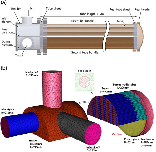
The heat exchangers are two-pass design, i.e. each heat exchanger includes two tube bundles. Each tube bundle has 230 tubes of length of 5.0 m. As the simulations will be focused on the fluid flow and particle motion in the inlet plenum and the downstream region from the tube entrance, the outlet plenum was ignored and the bottom/second tube bundle was modeled by a thin porous media with a near semi-circle geometry, i.e. the porous plate shown in Figure 1 b, in the refined model. Each tube in the top/first tube bundle was simplified to a short (400 mm) tube plus a porous plug (200 mm), as shown in Figure 1 b. The parameters of the 200 mm porous medium were determined by modeling the fluid flow through a tube of length of 4.6 m under different conditions, which can produce the same flow resistance as flowing through the full-scale tubes in the practical heat exchanger as shown in Figure 1 a. The importance of this approach is that there is no need to perform the high-cost simulations of full-scale heat exchangers, but the fluid flow and particle motion in the regions of interest can still be properly simulated with the model.

The entire geometry of the heat exchangers was considered in the present physical model. Another important difference of the present developed model to the previous approaches that have been used in the simulation of complex commercial heat exchangers is the inclusion of the rear plenum and simplifying the second tube bundle by a semi-circle plane. The reasons for this unique consideration will be discussed with the simulation results. One may concern that the models of HE1 and HE2 could be further simplified by only considering one half of the heat exchangers, if the flow through the symmetrical geometries is assumed to be symmetrical. Asymmetrical flow field has been observed in both experimental and numerical studies of the flow through sudden symmetric expansions (Sugawara et al., 2005; Ternik, 2009). Asymmetric flow in an inlet plenum has also been reported for a tubular heat exchanger (Bremhorst & Brennan, 2011), which has a side inlet nozzle similar to HE1. The flow characteristics can be ascribed to the enhancement of shear thinning behavior and its effect on the dimensions of the corner vortices and dead zones.

The heat exchanger model includes three inlet pipes, as shown in Figure 1. The interfaces between the inlet nozzles and the plenum were initially defined as walls. In the simulation of the heat exchanger (HE1, HE2 or HE3), the corresponding interface was changed to interior to let the fluid pass through. Therefore, the three heat exchangers shared the same meshes. This method aims to eliminate the difference in the simulation results that were generally caused by different meshes, even though a mesh independence study was conducted. This is important for the comparison of fluid flow, particle motion and metal erosion of the three heat exchangers. Figure 1 also shows the surface mesh scheme and specifically illustrates the tube configuration and the mesh topologies of the tube sheet and tubes. The mesh size used for the tube sheet and tube faces is 0.6 mm. Inflation layer meshing method was used in the tubes, the plenum and the inlet pipes to accurately capture the turbulent flow features and particle behaviors in the boundary layers. The growth ratio and the layer number are 1.2 and 5 respectively. The height of the first layer is 4.5 mm for the plenum and the pipes, but 0.1 mm was used for the tubes. The fluid domain of the inlet nozzles and plenum is of unstructured tetrahedral meshes with varying sizes in the range of 0.8–20 mm. The meshes were also refined by adopting a solution-adaptive mesh refinement procedure. The total meshes consist of 11.4 × 10⁶ cells and 25.9 × 10⁶ faces. The above-mentioned mesh scheme and mesh sizes were based on the grid-independence study. The grid dependence study by Bremhorst and Brennan (Bremhorst & Brennan, 2011) suggested a larger mesh size (3.75 mm) for the tube plate and tube inlets.

Multiphase flow

The water flow was described by the Reynolds–Averaged Navier–Stokes (RANS) equations. The turbulence model is significant for the case, where separating and recirculating flows may occur in the inlet plenum. The sudden expansion in flow space from the inlet nozzles to the plenum and the rapid contraction from the plenum to the tubes are most likely to produce adverse pressure gradients in the flow direction and the flow separation. It has been demonstrated that the SST-k-ω turbulence model can produce accurate and reliable results for a wide range of industrial turbulent problems (Menter et al., 2003; Versteeg & Malalasekera, 2007). Different turbulent models were compared for modeling particle behaviors in cyclone separators (Utikar et al., 2010), showing the standard k-ϵ turbulence model is not able to accurately simulate the flow with particle separation. The RANS and LES approaches are feasible for the simulation of this kind of industrial problems. Moreover, the model is capable of solving the turbulence in the region very close to the wall. This is most important for the present problem, where accurately capturing the features of flow and particles impacting on the tube sheet and the inside walls of the tubes is crucial for modeling the erosion. In this model, the turbulent viscosity (µ_t) is calculated by: (1) ${\mu }_t=\frac{\rho k}{\text{max}\left(\frac{\omega }{a^{\ast }},\frac{S{F}_2}{a_1}\right)}$(1) where, ρ is the fluid density; k is turbulent kinetic energy; ω is specific dissipation rate; a* and a₁ are model coefficients equal to 1 and 0.3; S is the mean strain rate tensor and the turbulent Prandtl numbers σ_k and σ_ω for k and ω are defined as: (2) $\begin{array}{rl}{\sigma }_k& =\frac{1}{\frac{F_1}{{\sigma }_{k,1}}-\frac{(1-F_1)}{{\sigma }_{k,2}}}\end{array}$(2) (3) $\begin{array}{rl}{\sigma }_w& =\frac{1}{\frac{F_1}{{\sigma }_{w,1}}-\frac{(1-F_1)}{{\sigma }_{w,2}}}\end{array}$(3) F₁ and F₂ are given by (4) $\begin{array}{rl}{F}_2& =\tanh \left({\left[max\left(\frac{2\sqrt{k}}{0.09\omega y},\frac{500\mu }{\rho y^2\omega }\right)\right]}^2\right)\end{array}$(4) (5) $\begin{array}{rl}{F}_1& =\tanh ([min(max\left(\frac{\sqrt{k}}{0.09\omega y},\frac{500\mu }{\rho y^2\omega }\right),\\ & {\frac{4\rho k}{{\sigma }_{\omega ,2}{D}_{kw}^{+}{y}^2})]}^4)\end{array}$(5) where, µ is the fluid viscosity; y is distance to the wall; the cross-diffusion coefficient, $D_{kw}^{+}$, is defined as: (6) $D_{kw}^{+}=max\left(2\rho \frac{1}{{\sigma }_{\omega ,2}\omega }\mathrm{\nabla }k\mathrm{\nabla }\omega ,{10}^{-10}\right)$(6) The three pipes have a diameter of 275 mm and a length of about 500 mm. They are too short to produce a fully developed flow for a fluid. The turbulent velocity profile over the inlet boundary was then approximated by the one-seventh power law. The turbulent intensity of 10% was specified for the inlet, while the value of the pipe diameter was applied for the turbulent length scale.

The transport of particles can be simulated by Lagrangian–Eulerian (LE) approach and CFD-CEM method, such as, Badr et al. (Badr et al., 2006) used LE method to track particles in an air-cooled heat exchanger, Greifzu et al. (Greifzu et al., 2016) assessed LE approach in modeling particle motion in incompressible, turbulent flow with OpenFOAM and ANSYS FLUENT, Chen et al. (Chen et al., 2020) used CFD-DEM method in the simulation of slurry transport in a pipeline, and Huang et al. (Huang et al., 2015) used CFD-DEM to analyze the transient solid–liquid flow in a centrifugal pump. The well-known Lagrangian particle tracking method has been used for various dilute systems, where trajectories of a finite number of dispersed particles were solved from their transient momentum, as described as Eqs (7) and (8). The velocity vector, position and concentration of particles were then obtained timely. In the present work the drag force for smooth spherical particles, the gravity, the virtual mass force at added mass coefficient of 1, and the force due to local pressure gradient were included in the particle transport equation as shown in Equation (9), since the densities of sand particles and fluid in the dilute water-particle flow are in the same order of magnitude. (7) $\begin{array}{rl}{m}_p\frac{d\overrightarrow{u_P}}{dt}& ={\sum }^{F_i}\end{array}$(7) (8) $\begin{array}{rl}\frac{d\mathit{r}}{dt}& =\overrightarrow{u_P}\end{array}$(8) where, m_p is the particle mass; r is the particle position; $\overrightarrow{u_P}$ is the particle velocity. The term $\sum F_i$ represents the sum of all forces on particles, which include the drag force, F_D, the gravity, F_B, the local pressure gradient force F_pg, and the virtual mass force, F_vm in the present work. (9) $\sum F_i=F_D+F_G+F_{pg}+F_{vm}$(9) These forces were calculated as follows in the simulations. (10) $\begin{array}{rl}{F}_D& =\frac{3\rho m_p}{4{\rho }_p{d}_p}{C}_D(\overrightarrow{u}-\overrightarrow{u_P})|\overrightarrow{u}-\overrightarrow{u_P}|\end{array}$(10) (11) $\begin{array}{rl}{F}_G& =\frac{({\rho }_p-\rho )\pi d_p^3}{6}\overrightarrow{g}\end{array}$(11) (12) $\begin{array}{rl}{F}_{pg}& =\frac{1}{6}\pi \rho d_p^3\overrightarrow{u_p}\mathrm{\nabla }\overrightarrow{u}\end{array}$(12) (13) $\begin{array}{rl}{F}_{vm}& =\frac{1}{12}\pi \rho d_p^3\left(\overrightarrow{u_p}\mathrm{\nabla }\overrightarrow{u}-\frac{d\overrightarrow{u_p}}{dt}\right)\end{array}$(13) where, ρ and ρ_p are the fluid density and the particle density, respectively; d_p is the particle diameter; $\overrightarrow{u}$ and $\overrightarrow{u_p}$are the fluid phase velocity and the particle velocity, respectively.

The particle dispersion due to turbulent velocity fluctuation was also described by a stochastic method, known as discrete random walk (DRW) model. The time-averaged velocity was from the RANS calculation. The DRW model assumes the fluctuating velocity in the direction normal to the wall is isotropic, which overpredicts the deposition of small particles on the walls. The influence of particles on the fluid flow was therefore included into the calculation to compensate, at a certain extent, the inherent problem of the DRW method. The particles were assumed to be spherical, rigid, no collusion, no rotation, and no energy interaction each other.

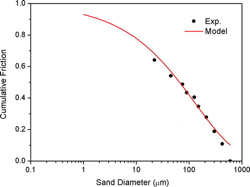
The particles were uniformly released from each cell of the inlet boundary after the fluid flow got ‘steady’. The particles are in the range of 1–500 µm and have a size distribution as shown in Figure 2. The size distribution was described by the logarithmic Rosin-Rammler formula. The mass rate of the particles injected into the heat exchangers was 0.01 kg/s. The particles were fed for 6 s at the same time step as the flow field simulation without particles.

Figure 2. Size distribution of sand particles in seawater utilized for a real-world heat exchanger. The measured data was described using the Rosin-Rammler function. The model was extended for the particles of 1–500 µm.

Solid particle impact erosion models

There are a few models for the prediction of the erosion, as discussed in the introduction. However, the accuracy of these models depends on the experimental conditions that were used in constructing the models. No general model is available for all conditions. In the present work the following general form of solid particle erosion model was used. (14) $R_e=\sum _{p=1}^N\frac{{\dot{m}}_{p}K{B}^{-n}{F}_s{f}_{\alpha }{u}_p^b}{A_f}{\left(\frac{d_p}{d_p^{\ast }}\right)}^m$(14) where, K is a material dependent constant; B is the Brinell hardness of wall; F_s is the particle sharpness factor and F_s = 0.2 was used for fully rounded sand particles; u_p is the particle velocity; d_p and $d_p^{\ast }$ are the particle diameter and the reference particle diameter, respectively, and d* = 326 µm was used for the seawater sand in the present modeling; A_f is the face area at the wall; n, b and m are empirical coefficients. f_α is a function of the particle impact angle, α, and is generally determined experimentally. The following function proposed by Oka et al (Oka & Yoshida, 2005) was used. The constants used in Eqs 14 and 15 are listed in Table 1. (15) $f(\alpha )=(\sin \alpha {)}^{n1}(1+H_V(1-sin\alpha ){)}^{n2}$(15) The erosion model expresses the dependence of erosion rate on both the physical (diameter, particle shape, density and material) and transport (impact angle and impacting velocity) properties of particles and the mechanical properties of target materials (hardness and material).

Table 1. Constants for erosion model

N	Fs	b	m	K	n1	n2
0.59	0.2	1.73	0.5	5.26E-5	0.7944	1.1292

Results and discussion

The erosion simulations of the heat exchangers were performed at the condition of water flow rate (210 × 10³ kg/h) and sand content (171 mg/kg). The sand particles were injected into the inlet nozzle at the same velocity as the water.

Fluid flow and particle motion in the plenum

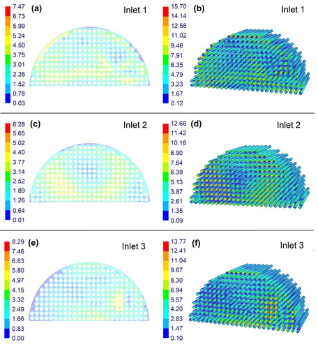
The flow in the inlet plenum of HE1 is asymmetrical as shown in Figure 3. This is due to the stronger recirculating flow in one half of the plenum, associating with a cross flow from one half of the plenum to the other half and a rotational flow in the inlet entrance. The particle trajectory traces captured by a high-speed digital camera (Habib et al., 2006) showed a flow pattern with one more swirl in the right half side of the tube entrance than the left half size, which well demonstrated the flow pattern simulated in this work. The simulation of gas flow in a similar heat exchanger (Bremhorst & Brennan, 2011) showed approximately symmetrical velocity and flow angle contours at tube sheet at a much higher flow rate than the present work. However, the large eddy simulations (LES) produced asymmetrical velocity and flow angle contours, instead of the symmetrical flow features. These flow features could not be revealed if only one half of the symmetrical domain of the heat exchanger were modeled. Inlet 2 produced an approximately symmetrical flow in the plenum. The expansion of flow occurred at a short region close to the tube sheet. In the plenum with inlet nozzle 3, the fluid flow towards to the forward half of the tube sheet and flow backwards to the near-nozzle region (Figure 3 g).

Figure 3. Path lines in the inlet plenum (a, d and g), velocity (b, e and h) and flow angle (c, f and i) of water close to the tube sheet. 90° denotes the flow direction is normal to the tube sheet.

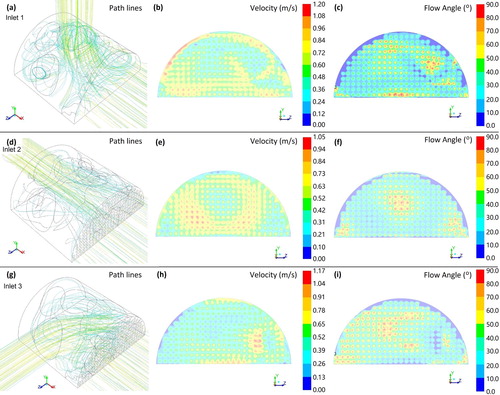
The erosion is a function of velocity, impact angle, hardness, shape, size and frequency (the number) of the particles impinging on the wall. For specified particles, their velocity, impact angle, size and frequency in a local cell depend on the fluid flow and the liquid–solid interaction. Both the particle behaviors and fluid flow features in the heat exchangers were then compared to reveal the difference in the erosion between the heat exchangers. The recirculating flow in the right (-z direction) half of the plenum of HE1 (Figure 3 a), the flow expansion in the plenum of HE2 (Figure 3 d) and the backward flow in the left half (+z direction) of the inlet plenum of HE3 (Figure 3 g) exhibit high velocity magnitude and low flow angle. Note that the flow angle is relative to the tube sheet plane. The comparison of the velocity contours indicates that inlet 2 produced the lowest local maximum velocity in the region near the tube sheet in HE2. The region with higher velocity in HE2 is larger than that in HE1 and HE3, where the high velocity regions are only in the left half corner of the head shell and the tube sheet (Figure 3 b) and in a small region on the right side near the tube sheet (Figure 3 h).

The sand impact angle is approximately consistent with the water flow direction. Solid particles having relatively low impact angle (about 10°–30°) will more likely result in the erosion. The experiments of erosion of carbon steel and copper by sand particles showed that the maximum erosion rate was at about 20° impact angle (Bitter, 1963a, 1963b). On the other hand, the kinetic energy of particles is a factor dominating the erosion rate. Beside the velocity and the number density of particles, the particle kinetic energy is also a function of particle size. The diameter and concentration distributions of particles were then analyzed in the next section.

Fluid flow and particle motion in the tubes

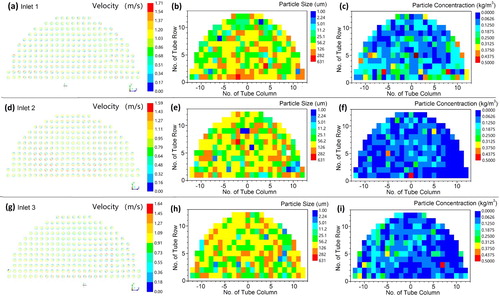
It is well known that the fluid flow pattern in the development region in the tubes associates with the velocity distribution at the entrance. Figure 4 a, d and g show the fluid velocity in the tube. The velocity in some tubes is obviously higher in one section than the other. These tubes are in the regions that have small flow angles as shown in Figure 3 c, f and i. In detail, the flow inclination occurs in most of the tubes of HE1 (Figure 4 a), in the tubes located at the circular fluid expansion region in HE2 (Figure 4 d) and in the bottom 2 row tubes and the tubes opening to the right backward flow region in HE3 (Figure 4 g). It was also found that the flow angle in the low velocity regions is lower, indicating the fluid flow towards the wall of the tubes. A comparison of the velocity distributions in the tubes of these heat exchangers (Figure 4 a, d and g) shows a lower flow inclination in HE2 and HE3 and less number of tubes with higher flow inclination angle in HE3.

Figure 4. Fluid velocity, mean diameter of particles and particle concentration in the tubes at 30 mm distance to the tube sheet.

To approach an optimum heat exchange in the device, uniform fluid distribution through the tube bundle is essential. The results show that the flow rate through a tube not only varies with the total fluid rate but also depends on the inlet nozzle and its location in the inlet plenum. The statistical results are given in Table 2, showing that HE2 produced more even fluid distribution through the first tube bundles, compared to HE1 and HE3. The difference of flow rates between the tubes of the first tube bundle is evident for each heat exchanger. The deviation of pressures at tube outlets in the rear plenum was also found, indicating the influence of flow in both the rear semi-spherical cover and the second tube bundle on the distribution of volumetric flow rates through the tubes of the first tube bundle. This nature cannot be captured when the heat exchanger model only includes the head and the first tube bundle. This is one of the main reasons why the rear plenum and the second tube bundle were considered in the present physical model.

Table 2. Statistical flow rates through tube bundles.

Items	HE1	HE2	HE3
Minimum (×10^−3 m^3/s)	0.2268	0.2338	0.2212
Maximum (×10^−3 m^3/s)	0.2922	0.2682	0.2821
(Max-Min)/Mean	0.2600	0.1367	0.2419
Coefficient of variation	0.0564	0.0316	0.0540

Note: The coefficient of variation represents the ratio of the standard deviation to the mean. It is used to compare the degree of variation from one tube bundle flow rate data series to another.

The particles entering tubes were statistically analyzed with respect to the average particle size and particle concentration. As can be seen from Figure 4 b, particle separation was predicted in the heat exchanger. Large particles tend to move to the bottom section of the inlet plenum and then enter the bottom two row tubes, while the fine particles move with fluid and go to the top of the plenum, as shown in Figure 5. The simulation results reported by Habib et al. (Habib et al., 2005) also showed that the particle distribution among the tubes and the location of eroded tubes greatly depend on the particle size and velocity, as well as predicted erosion only occurred on the tips of some tubes. They reported that large particles (200µm and 350µm) mainly caused the erosion with the tubes located at the bottom, while the fine particles (10µm) mainly caused the erosion of the peripheral tubes of the upper annular section, especially at the inlet flow velocity of less than 1.024 m/s.

Figure 5. Relative erosion rate (Re/Re*) caused by (a and c) fine particles (10µm) and (b and d) coarse particles (>300µm). (a) and (b) are the present simulation results. (c) and (d) are the results of a heat exchanger with 824 tubes and the maximum erosion rate Re* = 6.47 × 10⁻⁹ mg/g (Habib et al., 2005).

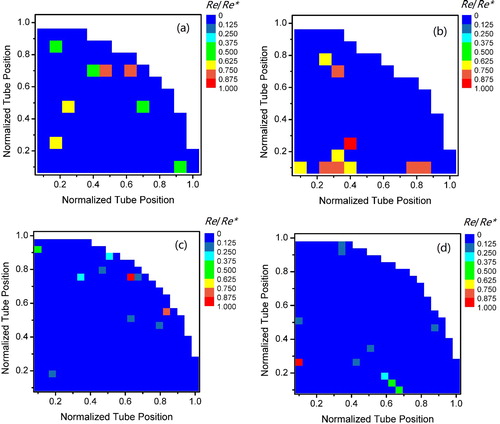
This behavior of large particles will cause fast erosion of the first-row tubes and the second-row tubes, which has been demonstrated practically in many industries. Note that the mean diameter of the injected sands is 130µm and the minimum size is 1µm. On the other hand, the small particles would facilitate the heat transfer in heat exchanger, as the nanofluids applied in various types of heat exchangers (Godson et al., 2014; Huminic & Huminic, 2012). It was reported that using the Ni/Water–glycerol nanofluid reduced the thermal resistance and led to the 100% improvement in heat exchanger performance (Ramezanizadeh et al., 2019). The fine particles suspended in base fluid would change the fluid thermal properties and reduce the thermal resistance at heat transfer surface, but the critical size of the particles that can enhance the heat transfer and not cause the metal erosion needs to be studied.

Obvious particle separation was not found in the inlet plenum of HE2 and HE3, as shown in Figure 4 e and h. There is no obvious sedimentation of sand particles in the tube entrance. This is unlike the behavior of particles in straight streamline flow. The sedimentation of 69 µm sand particles in water at a flow rate of 0.00315 m³/s in a straight horizontal tube with diameter of 3.02 cm was reported (Manzar & Shah, 2009). Whereas experiments showed that 70 µm copper particles were dispersed into a carrier fluid in an expansion channel (Greifzu et al., 2016). The fact that the particles did not sediment is attributed to the turbulent flow in the complex fluid domain and the very low sand volume concentration. However, the difference in the mean diameter exists between tubes, especially, between the tubes located on the bottom right-hand side corner (the 5th – 12^th columns of the 1^st – 6^th rows) of HE2 and the bottom and right-hand side tubes (the 1^st – 3^rd rows and the 5th – 10^th columns) of HE3. This is due to the change in flow direction and the recirculation of fluid in the corresponding regions in the inlet plenums (Figure 3 d and g). The difference may be also attributed to the low number of particles, as presented in Figure 4 f and i.

The particle separation in HE1 was also proved by the particle concentration in the tubes (Figure 4 c). The particle concentration in the 1st – 3^rd row tubes is higher than that in other tubes. Figure 4 f and i show that more particles enter the tubes that the fluid straightly flows into (as indicated by the flow paths shown in Figure 3). In the present work, the sand concentration of the seawater is about 0.171 kg/m³. A detailed inspection shows that inlet nozzle 1 caused the most uneven particle distribution through the tube bundle, whereas inlet nozzle 2 produced the most uniform particle distribution through tubes.

Shear stress

Shear stress is a tangential friction force produced by flowing fluid. The magnitude of shear stress depends on the fluid velocity and viscosity and, to a certain extent, it associates with erosion. The shear stress was thus used to evaluate the erosion in some investigations (Manzar & Shah, 2009). Then, the shear stresses on the tube sheet and the inside walls of tubes were calculated to identify the possible critical erosion locations.

The shear stress presented in Figure 6 is coincident with the flow profile shown in Figure 3, as it is only caused by fluid, i.e. no contribution from the solid particles. The velocity of fluid was regarded as zero, no slip condition, at wall boundaries, so that a laminar flow was produced close to the boundaries. This flow feature is caused by the friction of the fluid with the walls. The value of the friction associates with the fluid viscosity, the thickness of the laminar layer or sublayer, and the fluid velocity at the outer edge of the layer. When fluid flows within the heat exchangers, the thicknesses of the laminar layers near different walls are different and the fluid does not move at an identical velocity at the boundary layers. The shear stresses at different wall locations are therefore different.

Figure 6. Shear stress (unit: Pa) on the tube sheet (a, c and e) and the tubes (b, d and f).

Erosion rate and damage location

The erosion rate at a specific area in the heat exchangers is the mass loss of materials over time. Figure 7 shows the mass loss per unit area of tube sheet and tubes. Most walls have an erosion rate very lower than the highest value. So that the log scales were employed in Figure 7 to enable the difference in the erosion rate of most metal walls to be identified. Although the erosion is much relevant to the flow pattern, the velocity direction and the magnitude of sand particles are more important factors in the erosion. The separation of particles, especially large particles, from their original carrier fluid results in uneven particle distribution in the fluid, and the particles moving in different direction to the fluid flow path. The pattern of the erosion rate on the entire tube sheet and tubes is then different to that of the shear stress caused by viscous shear and turbulent shear shown in Figure 6. In detail, for example, high shear stresses were found in the region of the tube sheet around the 2^nd-4^th row (counted from the bottom) tubes in HE1, whereas high erosion occurred at the region of the tube sheet around the 1st and 2^nd row tubes. This indicates the essentiality of particle motion and erosion modeling in the investigation of heat exchanger failure. It was found that high erosion only occurs at scattered small areas. The simulations of erosion in a heat exchanges with 824 tubes (Habib et al., 2005) and in a heat exchanger with 38 tubes (Habib et al., 2006) also showed a location profile of the critical erosion tubes and the serious erosion only occurred on a few tubes.

Figure 7. Metal mass loss (×10⁶ mg/m²) of tube sheet and tubes in 3s at the areas having an erosion rate more than the average.

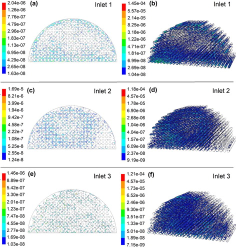
Figure 7 shows that HE1 has the most serious erosion on the tube sheet, and the maximum erosion rate of HE3 is the lowest. The results are also listed in Table 3. At the present there is no experimental results for this type of heat exchangers, as the online measurement of local erosion rate is still a challenge in practice. The rank of the heat exchangers by the tube erosion rate from lowest to highest is HE2, HE3 and HE1. The maximum erosion rates of tubes are much higher than these of the tube sheet. The average erosion rate of the tubes is a function of the length of the tubes used in the model. In the present physical model, the tubes are 400 mm in length. If longer tubes were employed in the modeling, the average erosion rate of the tubes would have decreased. The serious erosion, however, only happens on the tube surfaces close to the entrances. So that the maximum erosion rate is more significant in practice.

Table 3. Erosion rate, R_e, (mg/m² s) at tube sheet and tubes.

	Tube Sheet		Tubes
Heat Exchanger	Mean	Max	Mean	Max
HE1	5.45 × 10^−3	0.679	3.45 × 10^−3	48.2
HE2	4.14 × 10^−3	0.563	3.06 × 10^−3	39.3
HE3	3.43 × 10^−3	0.486	2.38 × 10^−3	40.4

HE2 shows the lowest fluid circulation in its inlet plenum (Figure 3 d), a relative uniform fluid velocity distribution near the tube sheet (Figure 3 e and f), and less particle separation in the inlet plenum. In the heat exchanger the largest particle concentration in fluid near the tube entrance is 15.6 kg/m³, which is much lower than 192 kg/m³ in HE1 and 287 kg/m³ in HE3. As a result, the particles were evenly distributed into the tubes (Figure 4 e and f), which avoided some metals continuously suffering impingement from large particles with high kinetic energy. The water flow in the tubes of HE2 is more even, having a lower level of the highest velocity and a straighter flow along the tubes, compared with HE1 and HE3 (Figure 4). These flow features finally resulted in lower shear stresses on the tubes in HE2 (Figure 6). The straight flow also implies a very low impact angle, at which the tube walls are unlikely to be eroded by the solid particles. All those together led to the low erosion in the heat exchanger (Figure 7).

Conclusions

The fluid flow, sea-sand motion and erosion in different two-pass copper tube heat exchangers were simulated to identify their critical erosion locations, predict the erosion rate and study the parameters that influence the solid particle erosion. The simulated results showed a reasonably good agreement with experimental and other simulation results. The critical erosion region of HE1 locates at the inlets of the 1st and 2nd row tubes and the inlets of the peripheral tubes of upper annular section. The mean erosion rate is about 5.5 × 10⁻³ mg/m² s at flow rate of 210 × 10³ kg/h and sand content of 171 mg/kg. The maximum erosion rate at the critical erosion position is up to 48.2 mg/m² s. The date of the critical erosion locations and the corresponding erosion rates of each heat exchanger are useful for estimating the service life of the heat exchangers and improving their structure.

The results showed the importance of the model for the simulation of erosion in the type of heat exchangers. The asymmetrical flow features, uneven flow rate distribution and other instabilities would not be captured by using the symmetrical model and the porous plug models, whereas the erosion greatly depends on these flow features. Capturing these features in modeling is important in terms of accuracy. A physical model was proposed in the present work. Each of long tubes of the first tube bundle was modeled by a short tube that has a length of 20 times of tube diameter and by a porous plug. The second tube bundle was also considered in the physical model using a porous plate medium. Beside the appropriate application of the RANS approach for this kind of industrial problems, the results showed the importance of this model in accurately modeling the flow field and particle behaviors in the inlet plenum and through the first tube bundle to properly predict the erosion. The model also enables the simulations of different heat exchangers to share the same meshes, which promised the comparability between the heat exchangers by reducing the mesh-dependence.

The comparison of the erosion of the tube sheet and tubes between the three heat exchangers showed that: HE1 exhibited the highest erosion rate at both the tube sheet and tubes; HE2 presented the lowest erosion rate at the tubes and lower erosion at the tube sheet; HE3 showed the lowest erosion rate at the tube sheet and approximately as the same erosion rate in the tubes as HE1. Compared to HE1, the maximum erosion rates of HE2 and HE3 are lower by about 17% and 28%, respectively, and the maximum tube erosion rates are lower by about 18% and 16%, respectively.

Although changing the inlet position can control the particle separation and alter the critical erosion locations, this may not significantly affect the erosion rate because the large and fine particles at the same solid volume concentration can result in approximately the same erosion rate. In the first heat exchanger, more large particles moved to the bottom section due to particle separation and more fine particles flow to the peripheral tubes of upper annular section with the carrier fluid, however there is no obvious difference in the erosion rate between the two critical locations.

The sand particles used in this work are from a seawater coolant. In practice seawater also contains various components that may cause the erosion, corrosion and fouling of heat exchangers, such as dissolved gases and organic compounds. The behavior of these substances in heat exchangers and how they work with sand to result in the erosion and corrosion of the tubes are unclear and need to be investigated in the future.

Disclosure statement

No potential conflict of interest was reported by the author(s).

Additional information

Funding

This work was supported by Hebei Province: [Grant Number E2019100007].

References

- Ahlert, K. R. (1994). Effects of particle impingement angle and surface wetting on solid particle erosion of AISI 1018 steel. BUniversity of Tulsa.
- Arabnejad, H., Mansouri, A., Shirazi, S. A., & McLaury, B. S. (2015). Development of mechanistic erosion equation for solid particles. Wear, 332–333, 1044–1050. https://doi.org/10.1016/j.wear.2015.01.031
- Aslam Bhutta, M. M., Hayat, N., Bashir, M. H., Khan, A. R., Ahmad, K. N., & Khan, S. (2012). CFD applications in various heat exchangers design: A review. Applied Thermal Engineering, 32(Complete), 1–12. https://doi.org/10.1016/j.applthermaleng.2011.09.001
- Badr, H. M., Habib, M. A., Ben-Mansour, R., Said, S. A. M., & Al-Anizi, S. S. (2006). Erosion in the tube entrance region of an air-cooled heat exchanger. International Journal of Impact Engineering, 32(9), 1440–1463. https://doi.org/10.1016/j.ijimpeng.2005.01.008
- Badr, H. M., Habib, M. A., Ben-Mansour, R., & Said, S. A. M. (2005). Numerical investigation of erosion threshold velocity in a pipe with sudden contraction. Computers & Fluids, 34(6), 721–742. https://doi.org/10.1016/j.compfluid.2004.05.010
- Batalha Leoni, G., Suaiden Klein, T., & de Andrade Medronho, R. (2017). Assessment with computational fluid dynamics of the effects of baffle clearances on the shell side flow in a shell and tube heat exchanger. Applied Thermal Engineering, 112, 497–506. https://doi.org/10.1016/j.applthermaleng.2016.10.097
- Bitter, J. G. A. (1963a). A study of erosion phenomena part I. Wear, 6(1), 5–21. https://doi.org/10.1016/0043-1648(63)90003-6
- Bitter, J. G. A. (1963b). A study of erosion phenomena: Part II. Wear, 6(3), 169–190. https://doi.org/10.1016/0043-1648(63)90073-5
- Bremhorst, K., & Brennan, M. (2011). Investigation of shell and tube heat exchanger tube inlet wear by computational fluid dynamics. Engineering Applications of Computational Fluid Mechanics, 5(4), 566–578. https://doi.org/10.1080/19942060.2011.11015395
- Bremhorst, K., & Lai, J. C. S. (1979). The role of flow characteristics in corrosion-erosion of tube inlets in the inlet channel of shell and tube heat exchangers. Wear, 54(1), 87–100. https://doi.org/10.1016/0043-1648(79)90048-6
- Campos-Amezcua, A., Mazur, Z., Gallegos-Muñoz, A., Romero-Colmenero, A., Riesco-Ávila, J. M., & Medina-Flores, J. M. (2007). Numerical study of erosion due to solid particles in steam turbine blades. Numerical Heat Transfer, Part A: Applications, 53(6), 667–684. https://doi.org/10.1080/10407780701453933
- Chen, J., Wang, Y., Li, X., He, R., Han, S., & Chen, Y. (2015). Erosion prediction of liquid-particle two-phase flow in pipeline elbows via CFD–DEM coupling method. Powder Technology, 275, 182–187. https://doi.org/10.1016/j.powtec.2014.12.057
- Chen, Q., Xiong, T., Zhang, X., & Jiang, P. (2020). Study of the hydraulic transport of non-spherical particles in a pipeline based on the CFD-DEM. Engineering Applications of Computational Fluid Mechanics, 14(1), 53–69. https://doi.org/10.1080/19942060.2019.1683075
- Finnie, I. (1972). Some observations on the erosion of ductile metals. Wear, 19(1), 81–90. https://doi.org/10.1016/0043-1648(72)90444-9
- Gandhi, M. S., Ganguli, A. A., Joshi, J. B., & Vijayan, P. K. (2012). CFD simulation for steam distribution in header and tube assemblies. Chemical Engineering Research and Design, 90(4), 487–506. https://doi.org/10.1016/j.cherd.2011.08.019
- Gao, W., Li, Y., & Kong, L. (2016). Numerical investigation of erosion of tube sheet and tubes of a shell and tube heat exchanger. Computers & Chemical Engineering, 96, 115–127. https://doi.org/10.1016/j.compchemeng.2016.10.005
- Godson, L., Deepak, K., Enoch, C., Jefferson, B., & Raja, B. (2014). Heat transfer characteristics of silver/water nanofluids in a shell and tube heat exchanger. Archives of Civil and Mechanical Engineering, 14(3), 489–496. https://doi.org/10.1016/j.acme.2013.08.002
- Greifzu, F., Kratzsch, C., Forgber, T., Lindner, F., & Schwarze, R. (2016). Assessment of particle-tracking models for dispersed particle-laden flows implemented in OpenFOAM and ANSYS FLUENT. Engineering Applications of Computational Fluid Mechanics, 10(1), 30–43. https://doi.org/10.1080/19942060.2015.1104266
- Habib, M. A., Badr, H. M., Ben-Mansour, R., & Kabir, M. E. (2007). Erosion rate correlations of a pipe protruded in an abrupt pipe contraction. International Journal of Impact Engineering, 34(8), 1350–1369. https://doi.org/10.1016/j.ijimpeng.2006.07.007
- Habib, M. A., Badr, H. M., Ben-Mansour, R., & Said, S. A. M. (2004). Numerical calculations of erosion in an abrupt pipe contraction of different contraction ratios. International Journal for Numerical Methods in Fluids, 46(1), 19–35. https://doi.org/10.1002/fld.744
- Habib, M. A., Badr, H. M., Said, S. A. M., Ben-Mansour, R., & Al-Anizi, S. S. (2006). Solid-particle erosion in the tube end of the tube sheet of a shell-and-tube heat exchanger. International Journal for Numerical Methods in Fluids, 50(8), 885–909. https://doi.org/10.1002/fld.1083
- Habib, M. A., Ben-Mansour, R., Badr, H. M., Said, S. A. M., & Al-Anizi, S. S. (2005). Erosion in the tube entrance region of a shell and tube heat exchanger. International Journal of Numerical Methods for Heat and Fluid Flow, 15(2), 143–160. https://doi.org/10.1108/09615530510578429
- Huang, S., Su, X., & Qiu, G. (2015). Transient numerical simulation for solid-liquid flow in a centrifugal pump by DEM-CFD coupling. Engineering Applications of Computational Fluid Mechanics, 9(1), 411–418. https://doi.org/10.1080/19942060.2015.1048619
- Huminic, G., & Huminic, A. (2012). Application of nanofluids in heat exchangers: A review. Renewable and Sustainable Energy Reviews, 16(8), 5625–5638. https://doi.org/10.1016/j.rser.2012.05.023
- Karimi, S., Shirazi, S. A., & McLaury, B. S. (2017). Predicting fine particle erosion utilizing computational fluid dynamics. Wear, 376–377, 1130–1137. https://doi.org/10.1016/j.wear.2016.11.022
- Kesana, N. R., Grubb, S. A., McLaury, B. S., & Shirazi, S. A. (2013). Ultrasonic measurement of multiphase flow erosion patterns in a standard elbow. Journal of Energy Resources Technology, 135(3), 032905–032905. https://doi.org/10.1115/1.4023331
- Kesana, N. R., Throneberry, J. M., McLaury, B. S., Shirazi, S. A., & Rybicki, E. F. (2013). Effect of particle size and liquid viscosity on erosion in annular and slug flow. Journal of Energy Resources Technology, 136(1), 012901–012901. https://doi.org/10.1115/1.4024857
- Klein, U., Zunkel, A., & Eberle, A. (2014). Breakdown of heat exchangers due to erosion corrosion and fretting caused by inappropriate operating conditions. Engineering Failure Analysis, 43, 271–280. https://doi.org/10.1016/j.engfailanal.2014.03.019
- Kuźnicka, B. (2009). Erosion–corrosion of heat exchanger tubes. Engineering Failure Analysis, 16(7), 2382–2387. https://doi.org/10.1016/j.engfailanal.2009.03.026
- Laguna-Camacho, J. R., Vite-Torres, M., Gallardo-Hernández, E. A., & Vera-Cárdenas, E. E. (2013). Solid particle erosion on different metallic materials. In D. H. Pihtili (Ed.), Tribology in Engineering. InTech. https://doi.org/10.5772/51176.
- Lai, J. C. S., & Bremhorst, K. (1979). Control of corrosion-erosion of tube inlets of shell and tube heat exchangers. Wear, 54(1), 101–112. https://doi.org/10.1016/0043-1648(79)90049-8
- Lin, Z., Ruan, X., Zhu, Z., & Fu, X. (2014). Numerical study of solid particle erosion in a cavity with different wall heights. Powder Technology, 254, 150–159. https://doi.org/10.1016/j.powtec.2014.01.002
- Lin, Z., Zhang, Y., Li, Y., Li, X., & Zhu, Z. (2017). Prediction of particle distribution and particle impact erosion in inclined cavities. Powder Technology, 305, 562–571. https://doi.org/10.1016/j.powtec.2016.10.035
- Lindroos, M., Apostol, M., Kuokkala, V.-T., Laukkanen, A., Valtonen, K., Holmberg, K., & Oja, O. (2015). Experimental study on the behavior of wear resistant steels under high velocity single particle impacts. International Journal of Impact Engineering, 78(Supplement C), 114–127. https://doi.org/10.1016/j.ijimpeng.2014.12.002
- Lindroos, M., Ratia, V., Apostol, M., Valtonen, K., Laukkanen, A., Molnar, W., Holmberg, K., & Kuokkala, V.-T. (2015). The effect of impact conditions on the wear and deformation behavior of wear resistant steels. Wear, 328–329(Supplement C), 197–205. https://doi.org/10.1016/j.wear.2015.02.032
- Liu, X.-y., Zhang, J.-z., & Shan, Y. (2017). Investigation of the pressure drop inside a rectangular channel with a built-in U-shaped tube bundle heat exchanger. Engineering Applications of Computational Fluid Mechanics, 11(1), 96–110. https://doi.org/10.1080/19942060.2016.1245629
- López del Prá, C., Velasco, F. J. S., & Herranz, L. E. (2010). Aerodynamics of a Gas Jet entering the secondary side of a vertical shell-And-tube heat exchanger: Numerical analysis of anticipated severe accident SGTR conditions. Engineering Applications of Computational Fluid Mechanics, 4(1), 91–105. https://doi.org/10.1080/19942060.2010.11015301
- Mansouri, A., Arabnejad, H., Karimi, S., Shirazi, S. A., & McLaury, B. S. (2015). Improved CFD modeling and validation of erosion damage due to fine sand particles. Wear, 338–339, 339–350. https://doi.org/10.1016/j.wear.2015.07.011
- Mansouri, A., Arabnejad, H., Shirazi, S. A., & McLaury, B. S. (2015). A combined CFD/experimental methodology for erosion prediction. Wear, 332–333, 1090–1097. https://doi.org/10.1016/j.wear.2014.11.025
- Manzar, M. A., & Shah, S. N. (2009). Particle distribution and erosion during the flow of newtonian and non-newtonian slurries in straight and coiled pipes. Engineering Applications of Computational Fluid Mechanics, 3(3), 296–320. https://doi.org/10.1080/19942060.2009.11015273
- Menter, F., Kuntz, M., & Langtry, R. (2003). Ten years of industrial experience with the SST turbulence model. (Ed.), (Eds.). Proceedings of the 4th International Symposium on Turbulence, Heat and Mass Transfer.
- Molinari, J. F., & Ortiz, M. (2002). A study of solid-particle erosion of metallic targets. International Journal of Impact Engineering, 27(4), 347–358. https://doi.org/10.1016/S0734-743X(01)00055-0
- Naz, M. Y., Ismail, N. I., Sulaiman, S. A., & Shukrullah, S. (2015). Electrochemical and dry sand impact erosion studies on carbon steel. Scientific Reports, 5(1), 16583. https://doi.org/10.1038/srep16583
- Neilson, J. H., & Gilchrist, A. (1968). Erosion by a stream of solid particles. Wear, 11(2), 111–122. https://doi.org/10.1016/0043-1648(68)90591-7
- Njobuenwu, D. O., & Fairweather, M. (2012). Modelling of pipe bend erosion by dilute particle suspensions. Computers and Chemical Engineering, 42, 235–247. https://doi.org/10.1016/j.compchemeng.2012.02.006
- Oka, Y. I., Ohnogi, H., Hosokawa, T., & Matsumura, M. (1997). The impact angle dependence of erosion damage caused by solid particle impact. Wear, 203–204, 573–579. https://doi.org/10.1016/S0043-1648(96)07430-3
- Oka, Y. I., Okamura, K., & Yoshida, T. (2005). Practical estimation of erosion damage caused by solid particle impact: Part 1: Effects of impact parameters on a predictive equation. Wear, 259(1–6), 95–101. https://doi.org/10.1016/j.wear.2005.01.039
- Oka, Y. I., & Yoshida, T. (2005). Practical estimation of erosion damage caused by solid particle impact: Part 2: Mechanical properties of materials directly associated with erosion damage. Wear, 259(1–6), 102–109. https://doi.org/10.1016/j.wear.2005.01.040
- Parsi, M., Kara, M., Agrawal, M., Kesana, N., Jatale, A., Sharma, P., & Shirazi, S. (2017). CFD simulation of sand particle erosion under multiphase flow conditions. Wear, 376–377, 1176–1184. https://doi.org/10.1016/j.wear.2016.12.021
- Parsi, M., Najmi, K., Najafifard, F., Hassani, S., McLaury, B. S., & Shirazi, S. A. (2014). A comprehensive review of solid particle erosion modeling for oil and gas wells and pipelines applications. Journal of Natural Gas Science and Engineering, 21, 850–873. https://doi.org/10.1016/j.jngse.2014.10.001
- Peng, W., & Cao, X. (2016). Numerical prediction of erosion distributions and solid particle trajectories in elbows for gas–solid flow. Journal of Natural Gas Science and Engineering, 30, 455–470. https://doi.org/10.1016/j.jngse.2016.02.008
- Pereira, G. C., de Souza, F. J., & de Moro Martins, D. A. (2014). Numerical prediction of the erosion due to particles in elbows. Powder Technology, 261, 105–117. https://doi.org/10.1016/j.powtec.2014.04.033
- Postlethwaite, J., & Nešić, S. (2011). Erosion–corrosion in single- and multiphase flow. In R. W. Revie (Ed.), Uhlig's corrosion handbook (pp. 215–227). https://doi.org/10.1002/9780470872864.ch18.
- Prakash, S., Prabhakar, S., Kumar, M. S., & Annamalai, K. (2015). Design optimization of a heat exchanger header with inlet modifier. Journal of Chemical and Pharmaceutical Sciences, 7, 347–350. http://www.scopus.com/inward/record.url?eid=2-s2.0-84939446187&partnerID=40&md5=80332da18db6aa1ae9904bb1e1c230b0.
- Ramezanizadeh, M., Nazari, M. A., Ahmadi, M. H., & Chau, K.-w. (2019). Experimental and numerical analysis of a nanofluidic thermosyphon heat exchanger. Engineering Applications of Computational Fluid Mechanics, 13(1), 40–47. https://doi.org/10.1080/19942060.2018.1518272
- Selma, B., Désilets, M., & Proulx, P. (2014). Optimization of an industrial heat exchanger using an open-source CFD code. Applied Thermal Engineering, 69(1–2), 241–250. https://doi.org/10.1016/j.applthermaleng.2013.11.054
- Sugawara, K., Yoshikawa, H., & Ota, T. (2005). LES of turbulent separated flow and heat transfer in a symmetric expansion plane channel. Journal of Fluids Engineering, 127(5), 865–871. https://doi.org/10.1115/1.1988344
- Sun, B., Zhao, T., Li, L., Ren, Y.-y., & Li, W. (2019). Flow field uniformity analysis and structural optimization of coal pyrolysis heat exchanger. Engineering Applications of Computational Fluid Mechanics, 13(1), 417–425. https://doi.org/10.1080/19942060.2019.1602081
- Ternik, P. (2009). Planar sudden symmetric expansion flows and bifurcation phenomena of purely viscous shear-thinning fluids. Journal of Non-Newtonian Fluid Mechanics, 157(1–2), 15–25. https://doi.org/10.1016/j.jnnfm.2008.09.002
- Utikar, R., Darmawan, N., Tade, M., Li, Q., Evans, G., Glenny, M., & Pareek, V. (2010). Hydrodynamic simulation of cyclone separators. In H. W. Oh (Ed.), Computational fluid dynamics. InTech. https://doi.org/10.5772/7106.
- Uzi, A., Ben Ami, Y., & Levy, A. (2017). Erosion prediction of industrial conveying pipelines. Powder Technology, 309, 49–60. https://doi.org/10.1016/j.powtec.2016.12.087
- Versteeg, H. K., & Malalasekera, W. (2007). An introduction to computational fluid dynamics: The finite volume method. Pearson Education.
- Vieira, R. E., Mansouri, A., McLaury, B. S., & Shirazi, S. A. (2016). Experimental and computational study of erosion in elbows due to sand particles in air flow. Powder Technology, 288, 339–353. https://doi.org/10.1016/j.powtec.2015.11.028
- Wallace, M. S., Peters, J. S., Scanlon, T. J., Dempster, W. M., McCulloch, S., & Ogilvie, J. B., & American Society of Mechanical, E. (2000). CFD-Based Erosion Modelling of Multi-Orifice Choke Valves. (Ed.), (Eds.). Summer meeting, American Society of Mechanical Engineers; Fluids Engineering Division.
- Xu, L., Zhang, Q., Zheng, J., & Zhao, Y. (2016). Numerical prediction of erosion in elbow based on CFD-DEM simulation. Powder Technology, 302, 236–246. https://doi.org/10.1016/j.powtec.2016.08.050
- You, Y., Chen, Y., Xie, M., Luo, X., Jiao, L., & Huang, S. (2015). Numerical simulation and performance improvement for a small size shell-and-tube heat exchanger with trefoil-hole baffles. Applied Thermal Engineering, 89, 220–228. https://doi.org/10.1016/j.applthermaleng.2015.06.012
- Zhang, Y., Reuterfors, E. P., McLaury, B. S., Shirazi, S. A., & Rybicki, E. F. (2007). Comparison of computed and measured particle velocities and erosion in water and air flows. Wear, 263(1–6), 330–338. https://doi.org/10.1016/j.wear.2006.12.048