Computational approach to the turbulent boundary layer of a rotating porous cylinder with strong suction based on an algebraic turbulence model

Abstract

Many important technical systems operate according to the principles of momentum transfer, heat transfer and mass transfer near the surface of a cylinder rotating in a confined space. Numerical study of the Taylor–Couette flow with an imposed inward radial throughflow in the rotating inner cylinder demonstrates the possibility of flow stabilization to prevent large-scale vortices up to high rotation rates. The fluid is involved in rotation by the inner rotating cylinder only in a thin layer (boundary layer) near the cylinder surface with strong radial throughflow. Turbulence in the boundary layer may occur before the centrifugal instability, and there is a way to control the thickness of the layer as well as shear intensity and turbulence intensity near the surface of the rotating cylinder. The present work develops a compact and robust approach for the turbulent boundary layer calculation on the surface of a rotating cylinder based on an algebraic turbulence model. The generalized Cebeci–Smith model was supplemented with Richardson number-based corrections to address the centrifugal force action. It also generalized the correction used for accounting for wall suction. Analytical corrections and empirical coefficients of the model were tuned to reflect the coupled influence of the specific flow conditions. The approach, comprehensively verified in the preliminary research, was adapted to the desired geometric configuration and checked. The modified algebraic turbulent model was incorporated into an iterative calculation method developed especially for the case of axisymmetric boundary layers. The results of the algebraic turbulence model with different combinations of rotational speed and suction velocity agree well with the simulation results of the Reynolds stress turbulent model. The method proposed provides efficient practical engineering calculations and can be applied up to approaching the centrifugal instability in the boundary layer.

KEYWORDS:

• boundary layer
• numerical simulation
• rotating cylinder
• turbulence model
• wall suction

1. Introduction

Flow from the outside of a rotating permeable cylinder is of interest for a number of technical applications. Rotational filtration (Beaudoin & Jaffrin, 1989; Lee & Lueptow, 2004; Jaffrin & Ding, 2015; Ji et al., 2016; Motin et al., 2015; Wereley et al., 2002; Wilkinson & Dutcher, 2017; Zheng et al., 2019) is one typical example where filtration through a rotating cylindrical membrane increases the productivity of fine liquid cleaning and reduces membrane fouling. As the typical concentration of the solid phase in such applications is low, the analysis of the carrying liquid motion near a rotating filtering cylinder is a separate problem. Rotating cylinder cooling is also closely connected to the same kind of flow. The comprehensive review by Fénot et al. (2011) contains a database on surface heat transfer in a rotor–stator system for the case of an incompressible liquid in the annular gap. Different configurations of the Taylor–Couette flow between a rotating inner cylinder and a stationary outer cylinder have been considered, with the rotating cylinder being impermeable, while the more recent publication by Mochalin et al. (2020) contains results demonstrating that inward radial cross-flow through the entire porous or slotted surface of the rotating cylinder is able to increase the heat transfer efficiency by 1.5 times. Thus, study of the flow close to the surface of a rotating permeable cylinder is a topical research problem.

The flow outside a rotating cylinder is subjected to centrifugal instability, which results in a secondary vortical motion. In the case of the gap between coaxial impermeable cylinders, the primary instability appears at a low enough rotation rate in the form of the axisymmetric Taylor vortices, and a variety of subsequent transformations of the flow modes accompanies the further increase in rotational speed (Andereck et al., 1986). Laminar–turbulent transition in the gap flow occurs considerably later than the centrifugal instability against the background of the vortical motion (Andereck et al., 1986; Koschmieder, 1979). A superimposed radial throughflow with a permeable rotating cylinder stabilizes the gap flow, shifting the onset of Taylor vortices toward greater rotation rates (Chang & Sartory, 1967; Johnson & Lueptow, 1997; Kolyshkin & Vaillancourt, 1997; Min & Lueptow, 1994; Serre et al., 2008). Mochalin and Khalatov (2015) showed that the intensive inward radial throughflow can prevent the onset of vortices until very high rotation rates. Moreover, they found that the rotating fluid motion induced by rotation of the permeable cylinder, is concentrated only in some layers close to the surface of the cylinder with sufficient radial throughflow. Under the conditions considered, the stationary outer cylinder does not influence the flow near the rotating inner cylinder, which can be treated as a boundary layer on the surface of the rotating permeable cylinder. The boundary layer thickness depends on both the rotation rate and radial cross-flow rate.

It has also been shown (Mochalin & Khalatov, 2015; Mochalin et al., 2020) that the boundary layer can become turbulent before the onset of centrifugal instability and it is possible to control the turbulence intensity in the boundary layer, making it even greater than in the turbulent vortical flow at the same rotation rate as the impermeable cylinder. The flow mode near a rotating permeable cylinder is promising for practical use, for instance, in phase separation or surface cooling applications. Therefore, calculation of the turbulent boundary layer on a rotating permeable cylinder is necessary in the development and design of such devices.

Numerical simulation in Mochalin et al., (2020) is based on solving the full Reynolds-averaged Navier–Stokes (RANS) equations with application of the Reynolds stress transfer turbulence model. High-order approximation schemes are used on the low-Reynolds-number computational mesh (with very fine near-wall resolution). The numerical procedure is highly resource consuming and is not suitable for practical calculations. Thus, the goal of the present work is the substantiation of a simple and reliable approach to turbulent boundary layer calculation on the surface of a rotating permeable cylinder with intensive flow suction.

Modern engineering applications of boundary-affected fluid flows typically require consideration of additional complex factors which, in principle, can be captured by the latest computational fluid dynamics (CFD) techniques; however, the numerical simulation becomes extremely resource consuming and cannot be widely implemented. Examples can be found (e.g. Ghalandari et al., 2019; Salih et al., 2019) where additional complicating factors related to fluid–solid interaction have been successfully addressed by the elaboration of the calculation approaches based on methods requiring sufficiently lower recourses than those in the most general conventional CFD technologies.

We intend to elaborate on the robust calculation method for the turbulent boundary layer on the surface of a rotating porous cylinder with strong suction, based on a suitable algebraic turbulence model. The model should be properly adjusted, calibrated for the specific flow conditions and verified. In the absence of the necessary experimental database, calibration is supposed to be fulfilled by the results of the detailed numerical simulation based on the sufficiently general approach substantiated in previous research (Mochalin & Khalatov, 2015; Mochalin et al., 2020).

2. Basic numerical simulation

An approach to numerical simulation of the turbulent flow between concentric permeable cylinders, with the inner cylinder rotating, is described in Mochalin and Khalatov (2015) and verified by comparison to known direct numerical simulations (DNS) and experimental data. The simulation is based on the RANS equations for momentum transfer and continuity equation for an incompressible fluid. The Reynolds stresses transport equations are also included according to the Reynolds stress transfer model.

The finite volume procedure (Ferziger et al., 2002; Patankar, 1980) is the basis for discretization of the governing equations. The Quadratic Upstream Interpolation for Convective Kinematics (QUICK) scheme (Leonard, 1979), providing third order accuracy on the structured grid, is used for the convective terms with special care of monotonicity control and prevention of non-physical oscillations. The second order central-difference scheme described in Ferziger et al. (2002) is used for the diffusive terms. The Semi-Implicit Method for Pressure Linked Equations-Consistent (SIMPLEC) scheme (Van Doormaal & Raithby, 1984) is used to provide the pressure–velocity coupling. The values of all flow variables are stored at the cell centers (co-located difference template), and the Rhie–Chow correction (Rhie & Chow, 1983) is utilized to avoid possible non-physical oscillations in the predicted pressure field. A three-layer second order temporal discretization scheme is used for transient calculations with implicit time integration treatment. For the source-type terms of the governing equations, explicit treatment is utilized. An under-relaxation approach is used to control the convergence of the iterations and the Gauss–Seidel method is used to solve the linear equations. It is implemented with the ability to run in parallel.

A periodical fragment of the annular gap between a rotating inner cylinder and a stationary outer cylinder was considered in Mochalin and Khalatov (2015) as a computational domain. The outer cylinder is uniformly permeable (porous) with the normal (radial) velocity component specified through the boundary conditions. Two configurations of the inner rotating cylinder were analyzed: entirely porous and slotted (with longitudinal porous slots). For the first configuration, the axisymmetric assumption for flow was used, while for the slotted configuration three-dimensional flow was considered with the azimuthal periodicity angle of π/8. The axial periodicity step was chosen to be $2.1d$, where $d=R_2-R_1$ is the gap width, and $R_1,R_2$ are the radii of the inner and outer cylinders. The eligibility of the axial and azimuthal periodicity and the choice for the domain extents have been discussed in detail.

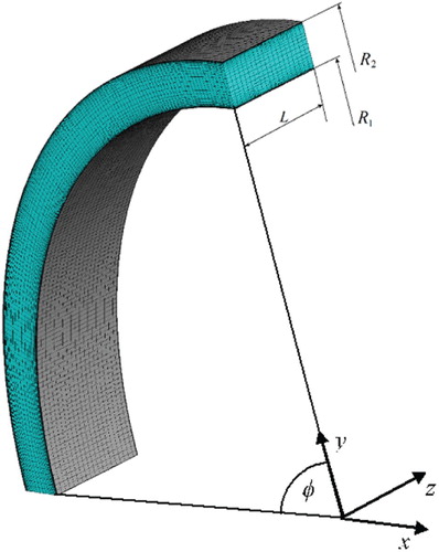
Our goal is to develop a numerical calculation approach for the turbulent boundary layer on the entirely porous cylinder surface. To obtain the necessary calibration database, we will use three-dimensional numerical simulation for the case of a uniformly porous inner cylinder. To achieve an acceptable computational time for conducting a large series of simulations, we will use azimuthal periodicity, taking the angular size of the computational segment to be $\pi /2$. This is represented in Figure 1, with the boundary surfaces meshed.

Figure 1. Meshed computational fragment of the flow domain.

We chose the aspect ratio $\mathrm{\Gamma }=d/L=2.1$, following Mochalin and Khalatov (2015), where it was discussed and shown that this forced value for the axial length of the vortex couple does not distort either the vortices onset boundary or characteristics of the turbulent vortical motion. In our analysis, the radius ratio was chosen as $\eta =R_1/R_2=0.9$. To choose the size of the computational mesh, we have fulfilled the check of grid independence for the numerical prediction of the significant integral flow parameters.

Before presenting the information on the grid-independence check, we note that the azimuthal and radial Reynolds numbers are significant dynamic parameters of the flow under consideration. They are defined as follows: ${\mathrm{R}\mathrm{e}}_{\phi }=W{R}_1/\nu =\mathrm{\Omega }{R}_1^2/\nu ,{\mathrm{R}\mathrm{e}}_r=V_s{R}_1/\nu$where $\mathrm{\Omega }$ is the angular velocity of the inner porous cylinder of radius $R_1$; $W,V_s$ are the azimuthal (rotational) velocity and normal (suction) velocity on its surface; and $\nu$ is the fluid kinematic viscosity. These parameters will be introduced in more depth in Section 3.

In Table 1 we present the calculated values of the integral friction coefficients ($C_{f1},C_{f2}$) for the inner and outer cylinders as well as the normalized average values of the velocity magnitude ($\overline{V}$) and vorticity magnitude ($\overline{\omega }$) in the domain. They are defined by the use of two meshes with different steps in the radial, azimuthal and axial directions ($n_r\times n_{\phi }\times n_z$). The azimuthal and radial Reynolds number values have been chosen to correspond to the large enough shear and suction rate.

Table 1. Integral flow parameters, calculated on different meshes, at ${\mathrm{R}\mathrm{e}}_{\phi }=1\cdot {10}^5,{\mathrm{R}\mathrm{e}}_r=400$.

$n_r\times n_{\phi }\times n_z$	$C_{f1}$	$C_{f2}$	$\overline{V}/W$	$\overline{\omega }/\mathrm{\Omega }$
35 × 112 × 20	0.007974	7.8355·10^−5	0.03103	8.75916
43 × 136 × 20	0.008014	7.8731·10^−5	0.03119	8.81172

It can been seen from Table 1 that the difference between the integral flow parameters is not more than 0.5% for the two meshes considered. Thus, for further calculation we use the mesh with 43 × 136 × 20 cells in the radial, azimuthal and axial directions, respectively. This mesh provides the value of the dimensionless wall coordinate $y^{+}<1$, for the cell centers in the mesh layer nearest to the rotating cylinder, up to ${\mathrm{R}\mathrm{e}}_{\phi }=2\cdot {10}^5$. For greater values, the mesh layer nearest to the wall is divided to maintain $y^{+}<1$. This is necessary for proper resolution of the laminar sublayer without using the wall functions, which are not suitable for cases of wall suction and streamlined curvature.

To check the validity of the numerical solution in its present realization, for the purpose of our analysis, we compared its prediction of the centrifugal instability boundary against the previously verified numerical results. The information on the flow mode (whether it is subcritical or Taylor-vortex flow) can be obtained by observing, in particular, the shape of the tangential velocity isosurface in the gap and the velocity vector plot in its axial cross-section. The corresponding examples are given in Figures 2 and 3.

Figure 2. (a) Isosurface of $V_{\phi }/W=0.2$ and (b) velocity vector plot in the plane $\phi =\pi /4$ for the case ${\mathrm{R}\mathrm{e}}_{\phi }=1\cdot {10}^5$, ${\mathrm{R}\mathrm{e}}_r=600$.

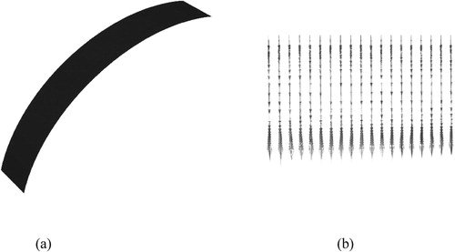
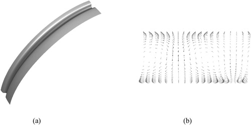
Figure 3. (a) Isosurface of $V_{\phi }/W=0.2$ and (b) velocity vector plot in the plane $\phi =\pi /4$ for the case ${\mathrm{R}\mathrm{e}}_{\phi }=1\cdot {10}^5$, ${\mathrm{R}\mathrm{e}}_r=300$.

For a fixed ${\mathrm{R}\mathrm{e}}_{\phi }$, there is a gap between the values of ${\mathrm{R}\mathrm{e}}_r$ corresponding to the onset and disappearance of the vortices. The possible size of the gap is influenced by the large relaxation time for centrifugal instability in a Taylor–Couette system (Czarny & Lueptow, 2007) and boundedness of the computational time. However, turbulence is also responsible, as the gap increases with the increase in ${\mathrm{R}\mathrm{e}}_{\phi }$. The two ${\mathrm{R}\mathrm{e}}_r$ values, corresponding to the onset and disappearance of the vortices, are called the lower and upper critical radial Reynolds numbers for a given ${\mathrm{R}\mathrm{e}}_{\phi }$. They are defined for the geometric configuration with the inner cylinder having axial porous slots as well as for the entirely porous inner cylinder surface. In the latter case, the axisymmetric approach was used. We defined the lower and upper critical ${\mathrm{R}\mathrm{e}}_r$ values in the present numerical simulation for several ${\mathrm{R}\mathrm{e}}_{\phi }$ and compared them to the corresponding results given in Mochalin and Khalatov (2015). The comparison is presented in Figure 4. The range between the lower and upper $({\mathrm{R}\mathrm{e}}_r{)}_{cr}$, taken from Mochalin and Khalatov (2015), includes all geometric configurations and modeling approaches considered in that work.

Figure 4. Centrifugal stability data comparison: 1–4 = ranges between lower and upper critical ${\mathrm{R}\mathrm{e}}_r$ values (numerical simulation of Mochalin and Khalatov, 2015) for $\eta =0.76,0.86$); 5 = linear neutral stability boundary (Mochalin & Khalatov, 2015); 6 = supercritical vortex flow (present numerical simulation for $\eta =0.9$); 7 = subcritical vortex-free flow (present numerical simulation for $\eta =0.9$).

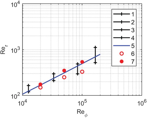
One can see the close correlation between our latest prediction and the known database. This validates the use of the numerical simulation approach presented here, in particular the collection of the necessary database on the flow in the gap between the stationary and rotating porous cylinders in the case of the subcritical flow mode with strong suction.

The stability data indirectly confirm the fact that fluid rotation at large enough suction can be concentrated in a boundary layer on the surface of the rotating inner cylinder, and the thickness of the boundary layer is less than the gap width. This is consistent with the fact that the stability boundary (the lower and upper critical radial Reynolds numbers) does not depend on the gap width (radius ratio $\eta$) when there is large enough suction. Indeed, centrifugal instability is formed within the rotating boundary layer and the gap width does not notably affect the transition.

The evolution of the boundary layer is displayed in Figure 5, where the profiles of the mean azimuthal velocity ($V_{\phi }$) and turbulence intensity ($Tu$) across the gap are presented for ${\mathrm{R}\mathrm{e}}_{\phi }=5\cdot {10}^4$ and three different subcritical ${\mathrm{R}\mathrm{e}}_r$ values.

Figure 5. Profiles of (a) turbulence intensity and (b) mean azimuthal velocity in the gap at ${\mathrm{R}\mathrm{e}}_{\phi }=5\cdot {10}^4$: 1 = ${\mathrm{R}\mathrm{e}}_r=500$; 2 = ${\mathrm{R}\mathrm{e}}_r=400$; 3 = ${\mathrm{R}\mathrm{e}}_r=350$.

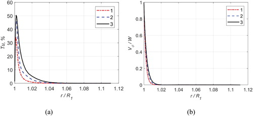
One can see an increase of about 50% in the thickness of the azimuthal velocity boundary layer (Figure 5b) and a 40% increase in the maximum value of the turbulent intensity (Figure 5a) when the radial Reynolds number (suction intensity) is reduced from ${\mathrm{R}\mathrm{e}}_r=500$ to ${\mathrm{R}\mathrm{e}}_r=350$. This emphasizes once more the possibility of controlling effectively the turbulent boundary layer on the surface of a rotating porous cylinder.

3. Analytical expression of the velocity profile

3.1. Basic assumptions and parameterization

We will consider, according to the preliminary discussion, a stable flow mode (before the onset of centrifugal instability) from the outside of a rotating porous cylinder of radius R₁. Rotational fluid motion is concentrated within a boundary layer of thickness $\delta$. The superimposed inward radial flow is usually referred to as suction in boundary layer studies. We suppose that the suction velocity $V_s$ has a uniform distribution over the cylinder surface. The flow is assumed to be unchanged in the axial direction ($V_z\equiv 0$, $\mathrm{\partial }/\mathrm{\partial }z\equiv 0$). The assumption of axial symmetry ($\mathrm{\partial }/\mathrm{\partial }\phi \equiv 0$) is also natural for the conditions under consideration.

We describe the fluid motion with the RANS equation for an incompressible liquid together with the continuity equation. A cylindrical reference frame $(r,\phi ,z)$ is used, with the z-axis directed along the rotating cylinder axis. The equation on projection in the azimuthal direction, under the above assumptions, can be written as (1) $\begin{array}{rl}\frac{\mathrm{\partial }}{\mathrm{\partial }r}\left(r{V}_r{V}_{\phi }\right)& =\frac{\mathrm{\partial }}{\mathrm{\partial }r}\left(r{\nu }_e\frac{\mathrm{\partial }{V}_{\phi }}{\mathrm{\partial }r}\right)+{\nu }_e\frac{\mathrm{\partial }{V}_{\phi }}{\mathrm{\partial }r}\\ & -r\frac{\mathrm{\partial }}{\mathrm{\partial }r}\left(\frac{{\nu }_e{V}_{\phi }}{r}\right)-\frac{2{\nu }_e{V}_{\nu }}{r}-V_{\phi }{V}_r\end{array}$(1) where $V_r,V_{\phi }$ are the radial and azimuthal mean velocity projections, $\rho$ is the liquid density, and ${\nu }_e$ is the effective kinematic viscosity, defined as the sum of the molecular viscosity ($\nu$) and the turbulent (or eddy) viscosity (${\nu }_t$).

The continuity equation in our case takes the form (2) $\frac{\mathrm{\partial }\left(r{V}_r\right)}{\mathrm{\partial }r}=0$(2) and we can integrate it with the condition $V_r\left(R_1\right)=V_s$ on the surface of the cylinder to obtain (3) $r{V}_r=const=-R_1{V}_s$(3) Equation (1) can be transformed, using (2), as follows: (4) $\begin{array}{r}\frac{\mathrm{\partial }}{\mathrm{\partial }r}\left(r^2{V}_r{V}_{\phi }\right)=\frac{\mathrm{\partial }}{\mathrm{\partial }r}\left(r^2{\nu }_e\frac{\mathrm{\partial }{V}_{\phi }}{\mathrm{\partial }r}-r{\nu }_e{V}_{\phi }\right)-r{V}_{\phi }\frac{\mathrm{\partial }{\nu }_e}{\mathrm{\partial }r}\end{array}$(4) Next, a stepwise calculation procedure is used, where the calculation domain across the boundary layer is divided into short pieces $\mathrm{\Delta }r$, and it is assumed that ${\nu }_e=const$ within each separate interval. It follows formally from this assumption that the last term in the right-hand part of Equation (4) can be neglected. This is an additional assumption and we follow it assuming that its validity will be apparent by testing our method in comparison with the detailed numerical simulation. Using equality (3) and the above assumptions, one can write the integral of (4) in the form (5) $-r{R}_1{V}_s{V}_{\phi }-r^2{\nu }_e\frac{\mathrm{\partial }{V}_{\phi }}{\mathrm{\partial }r}+r{\nu }_e{V}_{\phi }=C$(5) The constant C in Equation (5) can be defined using the following boundary condition at the rotating cylinder surface: (6) $r=R_1:V_{\phi }=\mathrm{\Omega }{R}_1=W,{\nu }_t=0,{\nu }_e=\nu$(6) The velocity gradient in (5) is expressed via the friction stress at the wall ${\tau }_w=|{\tau }_{r\varphi }{|}_{R_1}$ which, in the case of axial symmetry, can be presented as (7) ${\tau }_w=\left|\rho \nu {\left(\frac{\mathrm{\partial }{V}_{\phi }}{\mathrm{\partial }r}-\frac{V_{\phi }}{r}\right)}_{r=R_1}\right|$(7) Using the definition of friction velocity (Schlichting & Gerstan, 2016) $V_w=\sqrt{{\tau }_w/\rho }$, we can derive the following expression from formula (7) and the first of boundary conditions (6): (8) ${\left.\frac{\mathrm{\partial }{V}_{\phi }}{\mathrm{\partial }r}\right|}_{r=R_1}=-\frac{V_w^2}{\nu }+\frac{W}{R_1}$(8) On the basis of equalities (5), (6) and (8), we can write (9) $\begin{array}{r}-r{R}_1{V}_s{V}_{\phi }-r^2{\nu }_e\frac{\mathrm{\partial }{V}_{\phi }}{\mathrm{\partial }r}+r{\nu }_e{V}_{\phi }=-V_s{R}_1^{2}W+R_1^2{V}_w^2\end{array}$(9) To proceed to a dimensionless form, we take radius R₁ as a typical length and velocity W as a typical velocity. Dynamic head $\rho W^2$ will serve as a pressure scale. Then, the dimensional variables can be represented as (10) $r=R_1\xi ,V_r=W{u}_r,V_{\phi }=W{u}_{\phi },p=\rho W^{2}q$(10) where ξ is the dimensionless radial coordinate, $u_r,u_{\phi }$ are the dimensionless velocity projections, and q is the dimensionless pressure. Using (10), one can obtain the dimensionless form of Equation (9) as (11) $\begin{array}{rl}& -R^2{u}_s{W}^{2}r\xi u_{\phi }-R_{1}W(\nu +{\nu }_t){\xi }^2\frac{\mathrm{\partial }{u}_{\phi }}{\mathrm{\partial }y}\\ & +R_{1}W(\nu +{\nu }_t)\xi u_{\phi }=-u_s{R}_1^2{W}^2+R_1^2{W}^2{u}_w^2\end{array}$(11) where $u_w=V_w/W$ is the dimensionless friction velocity and $u_s=V_s/W$ is the dimensionless suction velocity. Dividing equality (11) by R₁W, one can rewrite it in the following form: (12) $\begin{array}{rl}& (1+{\tilde{\nu }}_t){\xi }^2\frac{d{u}_{\phi }}{dy}-(1+{\tilde{\nu }}_t)\xi u_{\phi }+u_s{\mathrm{R}\mathrm{e}}_{\varphi }\xi u_{\phi }\\ & =u_s{\mathrm{R}\mathrm{e}}_{\phi }-{\mathrm{R}\mathrm{e}}_{\phi }{u}_w^2\end{array}$(12) where ${\tilde{\nu }}_t={\nu }_t/v$ is the turbulent viscosity ratio and the rotational Reynolds number is defined as ${\mathrm{R}\mathrm{e}}_{\phi }=W{R}_1/v$. We will use also the radial Reynolds number ${\mathrm{R}\mathrm{e}}_r=V_s{R}_1/v=u_s{\mathrm{R}\mathrm{e}}_{\phi }$ for more general evaluation of the radial throughflow intensity. Both ${\mathrm{R}\mathrm{e}}_{\phi }$ and ${\mathrm{R}\mathrm{e}}_r$ have been already referenced in Section 2.

To solve Equation (12), we divide the computational domain across the boundary layer (in the normal direction to the surface of the rotating cylinder) into sufficiently small intervals $\mathrm{\Delta }{\xi }_i$, and within each the interval we consider the turbulent viscosity to be constant. This allows Equation (12) to be reduced in the interval to the form $\frac{d}{d\xi }\left((1+{\tilde{\nu }}_t){\xi }^{\frac{{\mathrm{R}\mathrm{e}}_r}{(1+{\tilde{\nu }}_t)}-1}{u}_{\phi }\right)=\left({\mathrm{R}\mathrm{e}}_r-{\mathrm{R}\mathrm{e}}_{\phi }{u}_w^2\right){\xi }^{\frac{{\mathrm{R}\mathrm{e}}_r}{(1+{\tilde{\nu }}_t)}-3}$resulting in the following integral: (13) $\begin{array}{r}(1+{\tilde{\nu }}_t){\xi }^{\frac{{\mathrm{R}\mathrm{e}}_r}{(1+{\tilde{\nu }}_t)}-1}{u}_{\phi }=\frac{\left({\mathrm{R}\mathrm{e}}_r-{\mathrm{R}\mathrm{e}}_{\phi }{u}_w^2\right)}{\left({\mathrm{R}\mathrm{e}}_r/(1+{\tilde{\nu }}_t)\right)-2}{\xi }^{\frac{{\mathrm{R}\mathrm{e}}_r}{(1+{\tilde{\nu }}_t)}-2}+C\end{array}$(13) Constant C can be defined with the use of the boundary condition (14) $u_{\phi }\left({\xi }_{0i}\right)=u_{\phi i}(i=1,2,\dots ,N)$(14) where ${\xi }_{0i},u_{\phi i}$ are the dimensionless radial coordinate and azimuthal velocity at the beginning of the interval $\mathrm{\Delta }{\xi }_i$. For the first step, it follows from (6) and (10) that ${\xi }_{01}=1,u_{\phi 1}=1$. Substituting (14) into equality (13), we obtain the following definition for constant C: (15) $\begin{array}{rl}C& =(1+{\tilde{\nu }}_t){\xi }_{0i}^{\left[\frac{{\mathrm{R}\mathrm{e}}_r}{(1+{\tilde{\nu }}_t)}-1\right]}{u}_{\phi i}\\ & -\frac{\left({\mathrm{R}\mathrm{e}}_r-{\mathrm{R}\mathrm{e}}_{\phi }{u}_w^2\right)}{\left({\mathrm{R}\mathrm{e}}_r/(1+{\tilde{\nu }}_t)\right)-2}{\xi }_{0i}^{\left[\frac{{\mathrm{R}\mathrm{e}}_r}{(1+{\tilde{\nu }}_t)}-2\right]}\end{array}$(15) Thus, in each interval $\xi \in [{\xi }_{0i},{\xi }_{0i}+\mathrm{\Delta }{\xi }_i]$ the azimuthal velocity, in accordance with equalities (13) and (15), is defined by the formula (16) $\begin{array}{rl}{u}_{\phi }& ={\left(\frac{{\xi }_{0i}}{\xi }\right)}^{\left[\frac{{\mathrm{R}\mathrm{e}}_r}{1+{\tilde{\nu }}_t}-1\right]}{u}_{\phi i}+\frac{{\mathrm{R}\mathrm{e}}_r-{\mathrm{R}\mathrm{e}}_{\phi }{u}_w^2}{{\mathrm{R}\mathrm{e}}_r-2(1+{\tilde{\nu }}_t)}\frac{1}{\xi }\\ & \times \left(1-{\left(\frac{{\xi }_{0i}}{\xi }\right)}^{\left[\frac{{\mathrm{R}\mathrm{e}}_r}{1+{\tilde{\nu }}_t}-2\right]}\right)\end{array}$(16)

3.2. Friction stress on the cylinder surface

Suction through the permeable surface delays the onset of vortices in the gap up to sufficiently high rotation rates for the flow mode under consideration. The radial Reynolds number (Re_r) can be so large in this case that the primary laminar velocity profile has the form (Mochalin & Khalatov, 2015) (17) $u_{\phi }={\xi }^{1-{\mathrm{R}\mathrm{e}}_r}$(17) For the normal derivative, from (17) we have the expression $\frac{\mathrm{\partial }{u}_{\phi }}{\mathrm{\partial }\xi }=\left(1-{\mathrm{R}\mathrm{e}}_r\right){\xi }^{-{\mathrm{R}\mathrm{e}}_r}$and for the local friction coefficient, (18) $c_f=\frac{{\tau }_w}{\left(\left(1/2\right)\rho W^2\right)}=2u_s$(18) Table 2 presents the friction coefficient values on the rotating cylinder surface under the conditions considered in this study. The values obtained numerically are matched to the results calculated by formula (18). For two ${\mathrm{R}\mathrm{e}}_{\phi },{\mathrm{R}\mathrm{e}}_r$ combinations from the table the flow is laminar, while for the others it is turbulent. Notably, the discrepancy in the application of formula (18) is not more than 1%. Based on this result, we assume that formula (18) is valid for the turbulent boundary layer under the conditions considered. This assumption leads to the following relationship: (19) $u_w^2=\frac{c_f}{2}=u_s$(19) Expression (19) allows formula (16) to be simplified to the form (20) $u_{\phi }={\left(\frac{{\xi }_{0i}}{\xi }\right)}^{\left[\frac{{\mathrm{R}\mathrm{e}}_r}{1+{\tilde{\nu }}_t}-1\right]}{u}_{\phi i}$(20)

Table 2. Friction coefficient values on the surface of a rotating cylinder with strong suction.

Rotational Reynolds	Radial Reynolds	Friction coefficient ($c_f$)
number (${\mathrm{R}\mathrm{e}}_{\phi }$)	number (${\mathrm{R}\mathrm{e}}_r$)	Numerical simulation	Formula (18)
5·10^4	1315	0.052939	0.0526
2·10^5	1315	0.013291	0.01315
2·10^5	2000	0.020064	0.02
3·10^5	2000	0.013398	0.013333
5·10^5	2500	0.010033	0.01

4. Algebraic turbulence model formulation

4.1. Basic relationships for turbulent viscosity

Wall suction is well known to be a stabilizing approach concerning the laminar–turbulent transition in a wall boundary layer (Araya et al., 2011; Ferro et al., 2017; Fransson et al., 2004; Kim et al., 2002; Schlatter & Örlü, 2011; Schlichting & Gersten, 2016; Trip & Fransson, 2014; Vigdorovich & Oberlack, 2008), but in our present consideration the suction is combined with other significant influencing factors, including the centrifugal force field and rotational symmetry. The numerical simulation we use is general enough to be suitable for the conditions mentioned, but our goal is to propose a more available and faster approach for use by a wider audience. Undoubtedly, algebraic turbulence models are the most accessible; they are conceptually simple and their application is not complex computationally. But they can provide, especially for boundary layer calculations, sufficient accuracy if applied within the limits of their calibration. The main idea follows from the above reasoning: to seek an appropriate basic algebraic turbulence model, to adjust it and calibrate for the conditions of the specific flow mode considered here. Because there is no experimental database for calibration, we will use the numerical simulation results obtained by the method presented above.

The development history of the Cebeci–Smith turbulence model (Cebeci & Chang, 1978; Cebeci & Smith, 1974) demonstrates a successful attempt at accounting for a number of additional complicated factors, namely, pressure gradient, wall suction (blowing), compressibility and low-Reynolds-number effects. It was possible to address each individual factor by introducing a separate correction multiplier (in the form of an empirical constant or expression containing empirics), while there is a coupled action of all the factors. Therefore, we take the generalized Cebeci–Smith model as a starting point in our analysis.

The base two-layer turbulence model proposed by Cebeci and Smith (1974) for planar flow can be formulated as follows: (21) $\begin{array}{rl}{\nu }_t& =\left\{\begin{array}{l}{\nu }_{ti},y\le y_m\\ {\nu }_{to},y>y_m\end{array}\right.\end{array}$(21) (22) $\begin{array}{rl}{\nu }_{ti}& =l_m^2{\left[{\left(\frac{\mathrm{\partial }{V}_x}{\mathrm{\partial }y}\right)}^2+{\left(\frac{\mathrm{\partial }{V}_y}{\mathrm{\partial }x}\right)}^2\right]}^{\frac{1}{2}}\end{array}$(22) (23) $\begin{array}{rl}{l}_m& =\kappa y\left(1-exp\left(-y^{+}/A_{\ast }\right)\right)\end{array}$(23) (24) $\begin{array}{rl}{\nu }_{to}& =k{V}_m{\delta }^{\ast }\end{array}$(24) (25) $\begin{array}{rl}{\delta }^{\ast }& ={\int }_0^{\delta }\left(1-\frac{V_x}{V_m}\right)dy\end{array}$(25) where ${\nu }_{ti},{\nu }_{to}$ are the kinematic coefficients of turbulent viscosity for the inner and outer regions of a turbulent boundary layer; $y_m$ is the lowest normal distance from the wall at which ${\nu }_{ti}={\nu }_{to}$; $V_x,V_y$ are the longitudinal and transversal velocity components; $l_m$ is the Prandtl mixing length; $y$ is the transversal (normal) coordinate counted from the wall; $V_m$ is the maximum velocity value in the boundary layer of thickness $\delta$; and ${\delta }^{\ast }$ is the displacement thickness of the boundary layer. The dimensionless wall coordinate is defined as (26) $y^{+}=\frac{V_{w}y}{\nu }$(26) The empirical constants have the values: (27) $\kappa =0.41,k=0.0168,A_{\ast }=26$(27) The generalization of the Prandtl formula (22) for the turbulent viscosity on an arbitrary near-wall flow can be written as follows: (28) ${\nu }_t=l_m^2\sqrt{2\dot{\mathbf{\text{S}}}\cdot \dot{\mathbf{\text{S}}}}$(28) where the convolution product of the strain rate tensor $\dot{\mathbf{\text{S}}}$ is under the root. One can derive formula (22), neglecting some terms in the expression (28), based on the estimation of the orders of magnitude proposed by Prandtl when deriving the boundary layer equations (Schlichting & Gersten, 2016).

The generalized Cebeci–Smith model (Cebeci & Smith, 1974) introduces some corrections to account for such additional factors as reduction in the turbulence intensity when approaching the boundary layer border, the effect of low Reynolds number on the turbulent viscosity in the outer region, wall suction (blowing), pressure gradient and fluid compressibility. We will not consider the last two in our case, but will incorporate the first three.

Reduction of the turbulent intensity in the proximity of the outer border is addressed using the Klebanoff intermittency coefficient: (29) $F_{kl}(y,\delta )={\left[1+5.5{\left(\frac{y}{\delta }\right)}^6\right]}^{-1}$(29) which is used as a multiplier in the right-hand side of Clauser’s formula (24).

Regarding correction of formula (24) for more accurate definition of the turbulent viscosity at low Reynolds numbers, the following representation of Clauser’s coefficient is introduced into the generalized Cebeci–Smith model: (30) $k=0.0168\frac{1.55}{1+{\mathrm{\Pi }}_0}$(30) where the wake parameter ${\mathrm{\Pi }}_0$ has been proposed by Schlichting and Gersten (2016) in the form (31) $\begin{array}{rl}{\mathrm{\Pi }}_0& =0.55\left(1-exp\left(-0,243\sqrt{z_1}-0.298z_1\right)\right),\\ z_1& =\frac{{\mathrm{R}\mathrm{e}}^{\ast \ast }}{425}-1\end{array}$(31) Reynolds number ${\mathrm{R}\mathrm{e}}^{\ast \ast }$ in formula (31) is defined as (32) ${\mathrm{R}\mathrm{e}}^{\ast \ast }=V_m{\delta }^{\ast \ast }/\nu$(32) by the boundary layer momentum thickness: (33) ${\delta }^{\ast \ast }={\int }_0^{\delta }\frac{V_x}{V_m}\left(1-\frac{V_x}{V_m}\right)dy$(33) The following correction to the empirical constant $A^{\ast }$ is introduced into formula (23) in the generalized Cebeci–Smith model to address the wall suction: (34) $A_{\ast }=26{\left(exp\left(C_1\frac{-V_s}{V_w}\right)\right)}^{-\frac{1}{2}},C_1=11.8$(34) Formula (34) is used instead of the constant value defined by the last equality in (27).

Streamline curvature (responsible for the appearance of centrifugal force) is not accounted for in the Cebeci–Smith model, so we need to introduce this factor in a separate approach, as it is very important for our consideration. A fruitful method was proposed by Bradshaw (1969) and has been used by many authors (Kikuyama et al., 1983; Nakamura et al., 1986; Reich & Beer, 1989; Weigand & Beer, 1992). It consists of the introduction of a correction multiplier into the expression for the definition of turbulent viscosity. The correction is based on the dynamic Richardson number (Ri), which describes the ratio between turbulent energy generation due to centrifugal force and that due to velocity gradient in shear turbulent flows: (35) ${\nu }_t={\nu }_{t0}(1-\text{β}\text{Ri}{)}^{2m}$(35) In the above formula, ${\nu }_{t0}$ is the turbulent viscosity defined without accounting for the streamline curvature and $\text{β},m$ are empirical constants. The choice of the empirical constants depends on the specifics of the shear flows used for calibration and we will consider this issue later. It is known the following expression for the Richardson number (Fransson et al., 2004) in the case of swirled flows with azimuthal and axial velocity components: (36) $\text{Ri = }\frac{2\left(V_{\phi }/r^2\right)\left(\mathrm{\partial }\right(V_{\phi }r\left)/\mathrm{\partial }r\right)}{{\left(\mathrm{\partial }{V}_z/\mathrm{\partial }r\right)}^2+{\left(\left(1/r\right)\left(\mathrm{\partial }\right(V_{\phi }r\left)/\mathrm{\partial }r\right)\right)}^2}$(36)

So, in the generalized Cebeci–Smith model, supplemented by the streamline curvature correction, expressions (22) and (24) for the turbulent viscosity in the inner and outer regions are replaced by the following formulas: (37) $\begin{array}{rl}{\nu }_{ti}& =l_m^2\sqrt{2\dot{\mathbf{\text{S}}}\cdot \dot{\mathbf{\text{S}}}}(1-\text{β}\text{Ri}{)}^{2m}\end{array}$(37) (38) $\begin{array}{rl}{\nu }_{to}& =k{\delta }^{\ast }{V}_m{F}_{kl}(1-\text{β}\text{Ri}{)}^{2m}\end{array}$(38) Coefficient $A_{\ast }$ in (23) needs defining by formula (34) and coefficient k in formula (38) is defined by formulas (30)–(33), instead of using the constant values specified in (27). The Klebanoff function $F_{kl}$ in (38) is defined by expression (29).

For planar axisymmetric fluid motion, the multiplier in (37), defining the mean flow velocity gradient, can be written as $\sqrt{2\dot{\mathbf{\text{S}}}\cdot \dot{\mathbf{\text{S}}}}={\left({\left(\frac{\mathrm{\partial }{V}_{\phi }}{\mathrm{\partial }r}-\frac{V_{\phi }}{r}\right)}^2+2{\left(\frac{\mathrm{\partial }{V}_r}{\mathrm{\partial }r}\right)}^2+2{\left(\frac{V_r}{r}\right)}^2\right)}^{\frac{1}{2}}$Using (3) and (10), we reduce it to (39) $\sqrt{2\dot{\mathbf{\text{S}}}\cdot \dot{\mathbf{\text{S}}}}=\frac{W}{R}{\left({\left(\frac{\mathrm{\partial }{u}_{\phi }}{\mathrm{\partial }\xi }-\frac{u_{\phi }}{\xi }\right)}^2+4{\left(\frac{u_s}{{\xi }^2}\right)}^2\right)}^{\frac{1}{2}}$(39) For normal distance y and universal wall coordinate y⁺ (26), we have, in our case: (40) $\begin{array}{rl}y& =r-R=R(\xi -1),\\ y^{+}& =\frac{u_{w}WR(\xi -1)}{\nu }=u_w{\mathrm{R}\mathrm{e}}_{\phi }(\xi -1)\end{array}$(40) Considering expressions (39) and (40), the definition of the turbulent viscosity in the inner region, given by formulas (37), (23) and (34), is as follows: (41) $\begin{array}{rl}{\tilde{\nu }}_{ti}& ={\kappa }^2(\xi -1{)}^2{\left(1-exp\left(\frac{-u_w{\mathrm{R}\mathrm{e}}_{\phi }(\xi -1)}{A_{\ast }}\right)\right)}^2\\ & \times {\mathrm{R}\mathrm{e}}_{\phi }{\left({\left(\frac{\mathrm{\partial }{u}_{{}^{\phi }}}{\mathrm{\partial }\xi }-\frac{u_{\phi }}{\xi }\right)}^2+4{\left(\frac{u_s}{{\xi }^2}\right)}^2\right)}^{\frac{1}{2}}\\ & \times (1-\text{β}\text{Ri}{)}^{2m}\end{array}$(41) (42) $\begin{array}{rl}{A}_{\ast }& =26exp\left(C_1\frac{u_s}{2u_w}\right)\end{array}$(42) The choice of empirical constants $\text{β},m,C_1$ will be discussed in Section 4.3.

For the Richardson number, from equality (36), considering $\xi \approx 1$, the following expression is obtained: (43) $\text{Ri}=2u_{\phi }/\left(\mathrm{\partial }{u}_{\phi }/\mathrm{\partial }\xi \right)$(43) As we have in our case $V_m=W$, the definition (38) of the turbulent viscosity in the boundary layer outer region transforms to the form (44) ${\tilde{\nu }}_{to}=k{\tilde{\delta }}^{\ast }{\mathrm{R}\mathrm{e}}_{\phi }{F}_{kl}(1-\text{β}\text{Ri}{)}^{2m}$(44) The dimensionless displacement thickness in (44) is defined as ${\tilde{\delta }}^{\ast }={\delta }^{\ast }/R_1$. The other dimensionless thicknesses $(\tilde{\delta },{\tilde{\delta }}^{\ast \ast })$ are defined in the same way. Coefficient k in (44) is defined by expressions (30) and (31) where, following from (32), we have (45) ${\mathrm{R}\mathrm{e}}^{\ast \ast }=\frac{W{\delta }^{\ast \ast }}{\nu }={\mathrm{R}\mathrm{e}}_{\phi }{\tilde{\delta }}^{\ast \ast }$(45) The Klebanoff intermittency coefficient, defined by formula (29), can be rewritten in the form (46) $F_{kl}={\left[1+5.5{\left(\frac{\xi -1}{\tilde{\delta }}\right)}^6\right]}^{-1}$(46) The problem considered has a specific feature which needs to be addressed when defining the displacement thickness; namely, the fact that the velocity profile typical for the boundary layer of a fixed surface takes place in the relative motion in the case being considered here. Therefore, one should define the displacement thickness by the relative velocity equaling $W-V_{\phi }$. Thus, Equation (25) in dimensionless form can be written as (47) ${\tilde{\delta }}^{\ast }={\int }_1^{1+\tilde{\delta }}{u}_{\phi }d\xi$(47) There is no need to introduce the relative velocity consideration when defining the momentum thickness. For any case, we have: (48) ${\tilde{\delta }}^{\ast \ast }={\int }_1^{1+\tilde{\delta }}{u}_{\phi }(1-u_{\phi })d\xi$(48)

4.2. Correction of the formula for turbulent viscosity in the outer region

The axisymmetric nature of the flow under consideration requires elaboration of a special algorithm for the boundary layer calculation. The conventional procedure is oriented toward a boundary layer being developed downstream, and the initial values of the necessary flow parameters are established at the starting cross-section. Then, the boundary layer thickness and the displacement and momentum thicknesses are taken from the previous cross-section when calculating the turbulent viscosity and the velocity profile in the next cross-section. This approach is justified because of the parabolicity of the conventional boundary layer equations in a longitudinal direction. An iterative procedure is required in our case, involving setting the initial approximations for the unknown quantities, including the boundary layer thicknesses, with their further correction from the results of the next calculation cycle. Convergence plays a key role in the implementation of the procedure. To study the issue, we will turn to the following reasoning. The velocity profiles presented in Figure 6 are typical for a stationary wall boundary layer and for a rotating cylinder boundary layer. The surface areas under the solid lines are specified as $S_1,S_2$, while those under the dashed lines are specified as $S_1^{\mathrm{\prime }},S_2^{\mathrm{\prime }}$. An increase in turbulent viscosity leads to greater exchange of momentum between the liquid layers, resulting in more occupied velocity profiles (dashed lines). The only difference is that for one case the profiles are concave while for the other they are convex. For a stationary surface, the geometric interpretation of formula (25) is ${\delta }_1^{\ast }=\frac{S_1}{V_m},{\delta }_1^{\mathrm{\prime }\ast }=\frac{S_1^{\mathrm{\prime }}}{V_m}$and for a rotating cylinder surface it has the form ${\delta }_2^{\ast }=\frac{S_2}{W},{\delta }_2^{\mathrm{\prime }\ast }=\frac{S_2^{\mathrm{\prime }}}{W}$One can see in Figure 6 that ${\delta }_1^{\mathrm{\prime }\ast }<{\delta }_1^{\ast }$ while ${\delta }_2^{\mathrm{\prime }\ast }>{\delta }_2^{\ast }$. Thus, overestimation of the initial value for the displacement thickness, giving overprediction of the turbulent viscosity in the outer region, leads, in the case of a stationary wall, to a lower calculated value of the displacement thickness, which is used in the next iteration. The calculated value of the displacement thickness is greater than its predicted value when the last is underestimated. So, there is a trend toward correcting the predicted value in the right direction in all cases for the fixed wall boundary layer. The opposite trend exists in the case of the rotating cylinder boundary layer when using formula (44).

Figure 6. Typical velocity profiles in the boundary layers on (a) a stationary surface and (b) a rotating cylinder surface: 1, smaller ${\nu }_t$ values; 2, greater ${\nu }_t$ values.

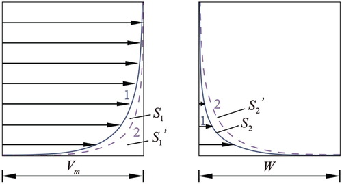
If a good estimation ${\tilde{\delta }}_0^{\ast }$ is known for the displacement thickness, one can use the following modification of expression (44): (49) ${\tilde{\nu }}_{to}=k\frac{{\left({\tilde{\delta }}_0^{\ast }\right)}^2}{{\tilde{\delta }}^{\ast }}{\mathrm{R}\mathrm{e}}_{\phi }{F}_{kl}(1-\text{β}\text{Ri}{)}^{2m}$(49) It follows from the above reasoning that convergence of the iterative procedure is restored in the case of using formula (49).

The displacement thickness depends on the velocity profile, which is defined by Equation (12). The form of the equation and equality (19) lead to the suggestion that the dimensionless displacement thickness depends mainly on two parameters: $u_s$ and ${\mathrm{R}\mathrm{e}}_{\phi }$. The detailed numerical simulation results can be used to establish the correlation ${\tilde{\delta }}_0^{\ast }(u_s,{\mathrm{R}\mathrm{e}}_{\phi })$. The values of the dimensionless boundary layer thicknesses for a number of combinations $u_s,{\mathrm{R}\mathrm{e}}_{\phi }$, from the range of the secondary vortical flows, are given in Table 3. The values of the dimensionless thicknesses were obtained from the numerical simulation presented in Section 2. Processing and analysis of the data obtained suggest the following correlation for the dimensionless displacement thickness: (50) $\begin{array}{rl}{\tilde{\delta }}_0^{\ast }(u_s,{\mathrm{R}\mathrm{e}}_{\phi })& =(5.9402\cdot {10}^{-12}-8.0321\cdot {10}^{-18}{\mathrm{R}\mathrm{e}}_{\phi })u_s^{-4}\\ & +7.0591\cdot {10}^{-9}{\mathrm{R}\mathrm{e}}_{\phi }-8.1935{\mathrm{R}\mathrm{e}}_{\phi }^{1/2}\\ & +2.3262\cdot {10}^{-3}\end{array}$(50) The correlation for the dimensionless boundary layer thickness, obtained by the data in Table 3, has the form: (51) $\begin{array}{rl}{\tilde{\delta }}_0(u_s,{\mathrm{R}\mathrm{e}}_{\phi })& =(2.7654\cdot {10}^{-13}-1.1217\cdot {10}^{-19}{\mathrm{R}\mathrm{e}}_{\phi })u_s^{-5}\\ & -2.3363\cdot {10}^{-8}{\mathrm{R}\mathrm{e}}_{\phi }+0.0105\end{array}$(51) One can use formulas (50) and (51) to choose the initial estimation of the corresponding dimensionless boundary layer thicknesses.

Table 3. Values of the dimensionless boundary layer thicknesses on the surface of a rotating suction cylinder.

Rotational	Dimensionless	Dimensionless	Dimensionless	Dimensionless
Reynolds number	suction velocity	boundary layer	displacement	momentum
(Reφ)	(us)	layer thickness ($\tilde{\delta }$)	thickness (${\tilde{\delta }}^{\ast }$)	thickness (${\tilde{\delta }}^{\ast \ast }$)
4.97607·10^4	6.5·10^−3	0.024	3.093·10^−3	1.539·10^−3
4.97607·10^4	7.0·10^−3	0.02229	2.89282·10^−3	1.44377·10^−3
4.97607·10^4	9.0·10^−3	0.01818	2.26545·10^−3	1.13433·10^−3
4.97607·10^4	9.5·10^−3	0.01818	2.13813·10^−3	1.06972·10^−3
1.99043·10^5	5.0·10^−3	0.08592	7.08057·10^−3	5.77247·10^−3
1.99043·10^5	6.575·10^−3	0.03871	2.61009·10^−3	2.00341·10^−3
1.99043·10^5	7.0·10^−3	0.02845	1.99553·10^−3	1.47678·10^−3
1.99043·10^5	9.0·10^−3	0.01253	7.9535·10^−4	4.8747·10^−4
1.99043·10^5	9.5·10^−3	5.064·10^−3	5.35872·10^−4	2.68662·10^−4
1.99043·10^5	0.01	5.064·10^−3	5.09054·10^−4	2.55257·10^−4
2.98564·10^5	5.0·10^−3	0.07976	5.51943·10^−3	4.61394·10^−3
2.98564·10^5	6.67·10^−3	0.02229	1.55317·10^−3	1.16976·10^−3
2.98564·10^5	7.0·10^−3	0.01818	1.27217·10^−3	9.31573·10^−4
2.98564·10^5	9.0·10^−3	6.334·10^−3	5.04397·10^−4	3.01921·10^−4
2.98564·10^5	9.5·10^−3	3.234·10^−3	3.57189·10^−4	1.79098·10^−4
2.98564·10^5	0.01	3.234·10^−3	3.39325·10^−4	1.70144·10^−4
4.97607·10^5	4.0·10^−3	0.09258	7.54272·10^−3	6.39332·10^−3
4.97607·10^5	5.0·10^−3	0.0695	3.77912·10^−3	3.22919·10^−3
4.97607·10^5	7.0·10^−3	0.01253	7.4078·10^−4	5.40076·10^−4
4.97607·10^5	9.0·10^−3	2.062·10^−3	2.26194·10^−4	1.1343·10^−4
4.97607·10^5	0.01	2.062·10^−3	2.03546·10^−4	1.02565·10^−4

The form parameter of the boundary layer $\left({\tilde{\delta }}_0^{\ast }/{\tilde{\delta }}_0^{\ast \ast }\right)$ varies, in the whole range considered of parameters $u_s,{\mathrm{R}\mathrm{e}}_{\phi }$, from 1.17 for the turbulent flow at the verge of the centrifugal instability to 2 for the laminar flow. For the first approximation, one can take a constant value for the form parameter and, in particular, use the equality: (52) ${\tilde{\delta }}_0^{\ast \ast }=0.625{\tilde{\delta }}_0^{\ast }$(52) Such a coarse approach is justified by the fact we are going to use it only for calculation at the first iteration.

Thus, relationships (49)–(52) allow the application of an iterative procedure for the axisymmetric boundary layer calculation and provide the first approximation for the boundary layer thickness, as well as for the displacement and momentum thicknesses.

4.3. Empirical factors for addressing the streamline curvature and flow suction

In the adopted model, streamline curvature and the influence of centrifugal mass forces on the turbulent exchange are accounted for via the Bradshaw correction (35), which is included in expressions (41) and (44) for the turbulent viscosity in the inner and outer regions. The most frequently used value for the empirical constant m is $m=1$. $\text{β}$ is often considered to be constant but generally it depends on the wall curvature, and our detailed numerical simulation shows that it also depends on the suction rate and rotation rate. The last factors are characterized by parameters $u_s$ and ${\mathrm{R}\mathrm{e}}_{\phi }$, and the boundary layer continuously transforms when the parameters are changed from a thin laminar layer to a significantly thicker turbulent layer. The correction is not necessary for the laminar layer, while its effect increases as the turbulence level increases. The turbulence level is connected to the value of form parameter ${\tilde{\delta }}_0^{\ast }/{\tilde{\delta }}_0^{\ast \ast }$, so one can try to express $\text{β}$ as a function of the form parameter. Test calculations corroborated the idea and calibration by the detailed numerical simulation gave the following expression for empirical coefficient $\text{β}$ in the Bradshaw correction: (53) $\text{β}=0.135{\left(\frac{{\tilde{\delta }}^{\ast }}{{\tilde{\delta }}^{\ast \ast }}-0.5\right)}^{-10}$(53) Flow suction in the base model is addressed by introducing an exponential multiplier into formula (41) for empirical constant $A_{\ast }$, defining the damping multiplier which corrects the ‘mixing length’ in the boundary layer inner region. The value of the multiplier depends on parameter $u_s$, addressing suction intensity, and on coefficient $C_1$. The constant value $(C_1=11.8)$ is used in the base Cebeci–Smith model for a plane wall. Testing of the model being developed demonstrated that $C_1$ in our case also mainly depends on the turbulence level in the boundary layer, which is tightly connected to the value of ${\tilde{\delta }}^{\ast }/{\tilde{\delta }}^{\ast \ast }$. In reality, there is zero turbulent viscosity value for the laminar layer $\left({\tilde{\delta }}^{\ast }/{\tilde{\delta }}^{\ast \ast }=2\right)$. To obtain ${\tilde{\nu }}_t=0$ from formulas (41) and (42), one should suppose that $C_1\to \mathrm{\infty }$. For the developed turbulent boundary layer, we have ${\tilde{\delta }}^{\ast }/{\tilde{\delta }}^{\ast \ast }\approx 1.17$ under the conditions considered here. The value $C_1\approx 11$ is known to be appropriate for a developed turbulent boundary layer. Calibration by the detailed numerical simulation gives the relationship (54) $C_1=5.35\cdot {10}^{-4}{\left(\frac{{\tilde{\delta }}^{\ast }}{{\tilde{\delta }}^{\ast \ast }}\right)}^{18.5}+11.217$(54) which correlates well with the two limit cases above.

We should note that the calibration procedures for factors $\text{β}$ and C₁ are coupled, as they both depend on the form parameter ${\tilde{\delta }}^{\ast }/{\tilde{\delta }}^{\ast \ast }$, and their choice, in turn, influences the form parameter value. The calibration database was created by numerical prediction of the form parameter. Values of ${\tilde{\delta }}^{\ast }/{\tilde{\delta }}^{\ast \ast }$ were defined for all potentially interesting ranges of parameters ${\mathrm{R}\mathrm{e}}_{\phi }$ and $u_s$ (or ${\mathrm{R}\mathrm{e}}_r$). Then, the test calculation were performed with the use of the approximate method being developed and different combinations of parameters $\text{β}$ and C₁ at each fixed combination of ${\mathrm{R}\mathrm{e}}_{\phi }$ and $u_s$. Variation of $\text{β}$ and C₁ was carried out according to the gradient descent method to minimize the difference between the form parameter value defined by the detailed numerical simulation and that defined by the method based on the algebraic turbulence model. Having sets of $\text{β}$ and C₁ values for the discrete set of the form parameter values, we chose suitable forms for the regression functions: $\text{β}\left({\tilde{\delta }}^{\ast }/{\tilde{\delta }}^{\ast \ast }\right)$, $C_1\left({\tilde{\delta }}^{\ast }/{\tilde{\delta }}^{\ast \ast }\right)$, and defined the corresponding coefficients by the least square method. The result is represented by formulas (53) and (54).

Wake parameter ${\mathrm{\Pi }}_0$ (expressions 31) in general also depends on the wall curvature, but in our case, it depends on the flow suction as well and both factors are addressed in an appropriate manner. So, one can use canonical representation (31) together with suitable choices of $\text{β}$ and $C_1$.

5. Calculation algorithm and testing

5.1. Iterative calculation procedure

Expression (25) for the dimensionless azimuthal velocity and the relationships obtained above defining the algebraic turbulence model make it possible to develop an iterative procedure for the boundary layer calculation on the surface of a rotating cylinder with suction of liquid. The main steps in the procedure are listed below.

1. The following quantities are specified as initial data:

   • rotational Reynolds number ${\mathrm{R}\mathrm{e}}_{\phi }$

   • dimensionless suction velocity $u_s$ (or radial Reynolds number ${\mathrm{R}\mathrm{e}}_r={\mathrm{R}\mathrm{e}}_{\phi }{u}_s$)

   • growing factor for the spatial step in the radial direction $k_r$

   • maximum allowable value for the dimensionless radial coordinate $\tilde{h}={\xi }_{max}$

   • tolerance of the dimensionless displacement thickness definition ${\epsilon }^{\ast }$.

2. One calculates:

   1. the value of dimensionless friction velocity $u_w$ from formula (19)

   2. the predicted value of dimensionless displacement thickness ${\tilde{\delta }}_0^{\ast }$ by formula (50)

   3. the predicted values of dimensionless thicknesses ${\tilde{\delta }}_0$ and ${\tilde{\delta }}_0^{\ast \ast }$ by formulas (51) and (52) respectively.

3. Quantities ${\tilde{\delta }}_0,{\tilde{\delta }}_0^{\ast },{\tilde{\delta }}_0^{\ast \ast }$ are taken as a first approximation for $\tilde{\delta },{\tilde{\delta }}^{\ast },{\tilde{\delta }}^{\ast \ast }$.

4. The dimensionless azimuthal velocity and radial coordinate at the first step are set as follows: $u_{\varphi 0}=1,{\xi }_{0,0}=1$

and the initial value of derivative $\mathrm{\partial }{u}_{\phi }/\mathrm{\partial }\xi$ is defined by the formula $(u_{\phi }{)}_{\left(\xi \right),0}=1-{\mathrm{R}\mathrm{e}}_{\phi }{u}_w^2,$which follows from equality (8) and definitions (10).

1. The length of the first near-wall step is defined from condition $y_1^{+}=0.5$ by the formula $\mathrm{\Delta }{\xi }_0={\xi }_1-1=\frac{y^{+}}{u_w{\mathrm{R}\mathrm{e}}_{\phi }}$

following from (26).

1. Wake parameter ${\mathrm{\Pi }}_0$, coefficient k, and coefficients $\text{β},C_1$ are defined by formulas (30), (31), (45), (53) and (54).

2. The following calculations are fulfilled in a cycle for the inner boundary layer region:

   1. for the values $\kappa =0.41$ and $m=1$, turbulent viscosity ratio ${\tilde{\nu }}_{ti}$ at the beginning of the current step is defined by formulas (41), (42) and (43)

   2. turbulent viscosity ratio ${\tilde{\nu }}_{to}$ corresponding to the outer region is calculated by formulas (43), (46) and (49)

   3. the lower of two values, ${\tilde{\nu }}_{ti},{\tilde{\nu }}_{to}$, is taken as the actual value of ${\tilde{\nu }}_t$

   4. coordinate ${\xi }_{1i}=min\left({\xi }_{0i}+\mathrm{\Delta }{\xi }_i,\tilde{h}\right)$ of the current step end is defined and the azimuthal velocity $u_{\phi (i+1)}$ at the step end is calculated by formula (25)

   5. derivative $\mathrm{\partial }{u}_{\phi }/\mathrm{\partial }\xi$ is defined at the step end as $(u_{\phi }{)}_{\left(\xi \right),i+1}=\left(u_{\xi (i+1)}-u_{\xi i}\right)/\mathrm{\Delta }{\xi }_i$

and the next step size $\mathrm{\Delta }{\xi }_{i+1}=min\left(\mathrm{\Delta }{\xi }_i\cdot k_r,0.1\left(\tilde{h}-1\right)\right)$

1. the condition is checked that the end of the internal region $\left({\tilde{\nu }}_t\ge {\tilde{\nu }}_{to}\right)$ has been reached, and if satisfied the calculation of the inner region is stopped; otherwise, operations of step (7) are repeated from (a).

(8)	The following operations are fulfilled in a cycle for the boundary layer outer region: the turbulent viscosity at the beginning of the current step is defined by formulas (30), (31), (43), (45), (46) and (49) the end of step coordinate is defined as ${\xi }_{i+1}=min\left({\xi }_i+\mathrm{\Delta }{\xi }_i,\tilde{h}\right)$ and the azimuthal velocity at the step end $\left(u_{\phi (i+1)}\right)$ is calculated by formula (25) derivative $\mathrm{\partial }{u}_{\phi }/\mathrm{\partial }\xi$ is defined at the step end as $(u_{\phi }{)}_{\left(\xi \right),i+1}=\left(u_{\phi (i+1)}-u_{\phi i}\right)/\mathrm{\Delta }{\xi }_i$and the next step size $\mathrm{\Delta }{\xi }_{i+1}=min\left(\mathrm{\Delta }{\xi }_i\cdot k_r,0.1\left(\tilde{h}-1\right)\right)$ calculation at the current iteration step is stopped in the case of reaching the end of the domain; otherwise, calculation is continued from the beginning of step (8).
(9)	Improved value $\tilde{\delta }$ is defined by relationship $u_{\phi }(1+\tilde{\delta })=0.001$, and corrected values ${\tilde{\delta }}^{\ast },{\tilde{\delta }}^{\ast \ast }$ are calculated by formulas (47) and (48).
(10)	The accuracy condition is checked in the form $|{\tilde{\delta }}_{i+1}^{\ast }-{\tilde{\delta }}_i^{\ast }|/max\left({\tilde{\delta }}_{i+1}^{\ast },{\tilde{\delta }}_i^{\ast }\right)\le {\epsilon }^{\ast }$. Calculation of the boundary layer is stopped when meeting the condition; otherwise, the iterations is continued from step (4).

5.2. Testing of the method

To validate the procedure, we compared the mean azimuthal velocity profiles and the profiles of the turbulent viscosity ratio calculated by the proposed algebraic turbulence model and by the detailed numerical simulation. The results for a number of different ${\mathrm{R}\mathrm{e}}_{\phi },{\mathrm{R}\mathrm{e}}_r$ combinations are presented in Figures 7 and 8. The analytical laminar profiles corresponding formally to the same ${\mathrm{R}\mathrm{e}}_r$ values and obtained by formula (17) have been added to these graphs. The combinations of parameters ${\mathrm{R}\mathrm{e}}_{\phi },{\mathrm{R}\mathrm{e}}_r$ were chosen in such a way as to examine the boundary layers from the thinnest laminar layer to the thickest turbulent layer close to the centrifugal instability border. It should be noted that the results presented in Figures 7 and 8 have been obtained for the parameter combinations which were not considered when calibrating the algebraic turbulence model.

Figure 7. Mean velocity profiles in the boundary layer on the surface of a rotating suction cylinder at (a) ${\mathrm{R}\mathrm{e}}_{\phi }=4.98\cdot {10}^4,{\mathrm{R}\mathrm{e}}_r=320$, (b) ${\mathrm{R}\mathrm{e}}_{\phi }=1.99\cdot {10}^5,{\mathrm{R}\mathrm{e}}_r=1310$, (c) ${\mathrm{R}\mathrm{e}}_{\phi }=2.99\cdot {10}^5,{\mathrm{R}\mathrm{e}}_r=2000$, (d) ${\mathrm{R}\mathrm{e}}_{\phi }=2.99\cdot {10}^5,{\mathrm{R}\mathrm{e}}_r=2700$, (e) ${\mathrm{R}\mathrm{e}}_{\phi }=4.98\cdot {10}^5,{\mathrm{R}\mathrm{e}}_r=2490$, and (f) ${\mathrm{R}\mathrm{e}}_{\phi }=4.98\cdot {10}^5,{\mathrm{R}\mathrm{e}}_r=4980$: 1 = numerical simulation, Reynolds stress transfer turbulence model; 2 = application of the algebraic turbulence model; 3 = laminar profile, formula (17).

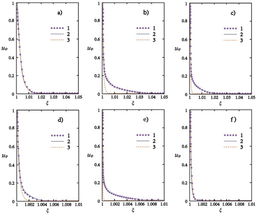
Figure 8. Turbulent viscosity ratio profiles at (a) ${\mathrm{R}\mathrm{e}}_{\phi }=4.98\cdot {10}^4,{\mathrm{R}\mathrm{e}}_r=320$, (b) ${\mathrm{R}\mathrm{e}}_{\phi }=1.99\cdot {10}^5,{\mathrm{R}\mathrm{e}}_r=1310$, (c) ${\mathrm{R}\mathrm{e}}_{\phi }=2.99\cdot {10}^5,{\mathrm{R}\mathrm{e}}_r=2000$, (d) ${\mathrm{R}\mathrm{e}}_{\phi }=2.99\cdot {10}^5,{\mathrm{R}\mathrm{e}}_r=2700$, (e) ${\mathrm{R}\mathrm{e}}_{\phi }=4.98\cdot {10}^5,{\mathrm{R}\mathrm{e}}_r=2490$, and (f) ${\mathrm{R}\mathrm{e}}_{\phi }=4.98\cdot {10}^5,{\mathrm{R}\mathrm{e}}_r=4980$: 1 = numerical simulation, Reynolds stress transfer turbulence model; 2 = application of the algebraic turbulence model; 3 = laminar profile, formula (17).

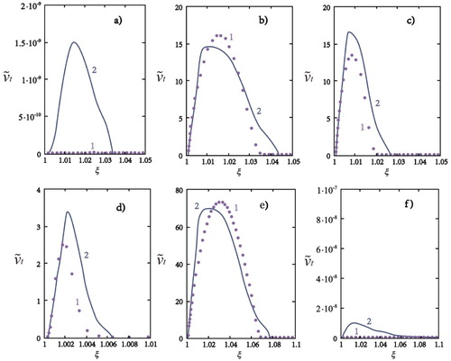
Comparative analysis shows that the elaborated procedure based on an algebraic turbulence model provides a definition of the azimuthal velocity profile which is practically the same as the profile predicted by the detailed numerical simulation with application of the differential Reynolds stress transport model. The proposed method is also able to reproduce the laminar velocity profile corresponding to sufficiently strong suction.

The algebraic turbulence model allows the real nature of the turbulent viscosity distribution in the boundary layer to be obtained, along with acceptable quantitative agreement with the results of more exact and complex computations. It provides evidence for, among other things, the admissibility of neglecting the term $r{V}_{\phi }\left(\mathrm{\partial }{\nu }_e/\mathrm{\partial }r\right)$ in Equation (4) to provide its explicit integration. Of course, we may conclude this only regarding the specific flow mode considered.

The results confirm that rotational fluid motion is concentrated within the boundary layer on the surface of the rotating cylinder at strong enough radial inflow. Turbulence and centrifugal instability develop in this layer with the increase in rotation amount (in terms of ${\mathrm{R}\mathrm{e}}_{\phi }$). A reduction in the inflow rate (${\mathrm{R}\mathrm{e}}_r$) at a fixed value of ${\mathrm{R}\mathrm{e}}_{\phi }$ is accompanied by an increase in the boundary layer thickness. The turbulent viscosity also grows within the layer. Centrifugal instability, resulting in large-scale vortices, arises notably later than the onset of turbulence in the boundary layer at large ${\mathrm{R}\mathrm{e}}_r$. Thus, through the combination of ${\mathrm{R}\mathrm{e}}_{\phi },{\mathrm{R}\mathrm{e}}_r$, one can control the boundary layer thickness and turbulence intensity within it, which can be used in many innovative practical applications.

6. Conclusions

A simple, fast and adequate approach to the turbulent boundary layer calculation on the surface of a rotating permeable cylinder has been elaborated for the case of strong suction through the cylinder surface. A two-layer algebraic turbulence model has been adjusted to account for the centrifugal force field (streamline curvature) and wall suction. Analytical corrections and empirical coefficients wer used to tune the model for the specific conditions of the coupled influence of these factors. To obtain the necessary calibration database, the numerical simulation approach, based on application of the Reynolds stress turbulence model and comprehensively verified in the preliminary research, was adopted to the desired geometric configuration and checked.

An iterative procedure developed for the boundary layer calculation is suitable for the axisymmetric nature of the boundary layer without its build-up along the streamline direction. The applicability limit of the method is the onset of vortices resulting in centrifugal instability, and it can be estimated from the stability diagram provided by Mochalin and Khalatov (2015). In the case of strong suction through the surface of a rotating cylinder, centrifugal instability can be postponed up to large rotation rates $({\mathrm{R}\mathrm{e}}_{\phi }\sim {10}^5)$, and by varying the radial throughflow rate one can control over a wide range the boundary layer thickness and turbulence intensity within it. This provides a way to control the amount of shear near the surface of a rotating cylinder as well as the intensity of momentum transfer, heat transfer and mass transfer. The proposed boundary layer calculation procedure supports the engineering calculation in possible practical applications of the flow under consideration. These include dynamic rotational filtration, and heat protection of rotors and shafts. Innovative designs of rotational heat exchangers and mass transfer installations can also be considered.

The method developed can easily be implemented in a simple code or script; it is fast and does not require any special qualifications to use. One should mention as well a limitation of the method, as it neglects the surface roughness of the rotating cylinder, which can be important in some cases. Analysis of the surface roughness effect is among the directions for further development of the present study.

Acknowledgements

The authors kindly acknowledge the support of the National Natural Science Foundation of China [grant number 51976251], Zhejiang Provincial Natural Science Foundation [grant number LY18E060006] and the National Undergraduate Innovation and Entrepreneurship Training Program of China [grant number 201910345049].

Disclosure statement

No potential conflict of interest was reported by the authors.

Additional information

Funding

The authors kindly acknowledge the support of the National Natural Science Foundation of China [grant number 51976251), Zhejiang Provincial Natural Science Foundation [grant number LY18E060006] and National Undergraduate Innovation and Entrepreneurship Training Program of China [grant number 201910345049].

References

- Andereck, C. D., Liu, S. S., & Swinney, H. L. (1986). Flow regimes in a circular Couette system with independently rotating cylinders. Journal of Fluid Mechanics, 164(3), 155–183. https://doi.org/10.1017/S0022112086002513
- Araya, G., Leonardi, S., & Castillo, L. (2011). Steady and time-periodic blowing/suction perturbations in a turbulent channel flow. Physica D: Nonlinear Phenomena, 240(1), 59–77. https://doi.org/10.1016/j.physd.2010.08.006
- Beaudoin, G., & Jaffrin, M. Y. (1989). Plasma filtration in Couette flow membrane devices. Artificial Organs, 13(1), 43–51. https://doi.org/10.1111/j.1525-1594.1989.tb02831.x
- Bradshaw, P. (1969). The analogy between streamline curvature and buoyancy in turbulent shear flow. Journal of Fluid Mechanics, 36(1), 177–191. https://doi.org/10.1017/S00221-12069001583
- Cebeci, T., & Chang, K. C. (1978). Calculation of incompressible rough-wall boundary-layer flows. AIAA Journal, 16(7), 730–735. https://doi.org/10.2514/3.7571
- Cebeci, T., & Smith, A. M. (1974). Analyses of turbulent boundary layers. Academic Press.
- Chang, T. S., & Sartory, W. K. (1967). Hydromagnetic stability of dissipative flow between rotating permeable cylinders. Journal of Fluid Mechanics, 27(1), 65–79. https://doi.org/10.1017/S0022112067000059
- Czarny, O., & Lueptow, R. M. (2007). Time scales for transition in Taylor-Couette flow. Physics of Fluids, 19(5), 054103. https://doi.org/10.1063/1.2728785
- Fénot, M., Bertin, Y., Dorignac, E., & Lalizel, G. (2011). A review of heat transfer between concentric rotating cylinders with or without axial flow. International Journal of Thermal Sciences, 50(7), 1138–1155. https://doi.org/10.1016/j.ijther-malsci.2011.02.013
- Ferro, M., Fallenius, B. E., & Fransson, J. H. (2017). On the turbulent boundary layer with wall suction. In R. Örlü, A. Talamelli, M. Oberlack, & J. Peinke (Eds.), Progress in turbulence VII (pp. 39–44). Springer.
- Ferziger, J. H., Perić, M., & Street, R. L. (2002). Computational methods for fluid dynamics. Springer.
- Fransson, J. H., Konieczny, P., & Alfredsson, P. H. (2004). Flow around a porous cylinder subject to continuous suction or blowing. Journal of Fluids and Structures, 19(8), 1031–1048. https://doi.org/10.1016/j.jfluidstructs.2004.06.005
- Ghalandari, M., Bornassi, S., Shamshirband, S., Mosavi, A., & Chau, K. W. (2019). Investigation of submerged structures’ flexibility on sloshing frequency using a boundary element method and finite element analysis. Engineering Applications of Computational Fluid Mechanics, 13(1), 519–528. https://doi.org/10.1080/19942060.2019.1619197
- Jaffrin, M. Y., & Ding, L. (2015). A review of applications of rotating and vibrating membranes systems: Advantages and drawbacks. Journal of Membrane and Separation Technology, 4(3), 134–148. https://doi.org/10.6000/1929-6037.2015.04.03.5
- Ji, P., Motin, A., Shan, W., Bénard, A., Bruening, M. L., & Tarabara, V. V. (2016). Dynamic crossflow filtration with a rotating tubular membrane: Using centripetal force to decrease fouling by buoyant particles. Chemical Engineering Research and Design, 106, 101–114. https://doi.org/10.1016/j.cherd.2015.11.007
- Johnson, E. C., & Lueptow, R. M. (1997). Hydrodynamic stability of flow between rotating porous cylinders with radial and axial flow. Physics of Fluids, 9(12), 3687–3696. https://doi.org/10.1063/1.869506
- Kikuyama, K., Murakami, M., Nishibori, K., & Maeda, K. (1983). Flow in an axially rotating pipe: A calculation of flow in the saturated region. Bulletin of JSME, 26(214), 506–513. https://doi.org/10.1299/jsme1958.26.506
- Kim, K., Sung, H. J., & Chung, M. K. (2002). Assessment of local blowing and suction in a turbulent boundary layer. AIAA Journal, 40(1), 175–177. https://doi.org/10.2514/2.1629
- Kolyshkin, A. A., & Vaillancourt, R. (1997). Convective instability boundary of Couette flow between rotating porous cylinders with axial and radial flows. Physics of Fluids, 9(4), 910–918. https://doi.org/10.1063/1.869187
- Koschmieder, E. L. (1979). Turbulent Taylor vortex flow. Journal of Fluid Mechanics, 93(3), 515–527. https://doi.org/10.1017/S0022112079002639
- Lee, S., & Lueptow, R. M. (2004). Rotating membrane filtration and rotating reverse osmosis. Journal of Chemical Engineering of Japan, 37(4), 471–482. https://doi.org/10.1252/jcej.37.471
- Leonard, B. P. (1979). A stable and accurate convective modelling procedure based on quadratic upstream interpolation. Computer Methods in Applied Mechanics and Engineering, 19(1), 59–98. https://doi.org/10.1016/0045-7825(79)90034-3
- Min, K., & Lueptow, R. M. (1994). Hydrodynamic stability of viscous flow between rotating porous cylinders with radial flow. Physics of Fluids, 6(1), 144–151. https://doi.org/10.1063/1.868077
- Mochalin, I., & Khalatov, A. (2015). Centrifugal instability and turbulence development in Taylor–Couette flow with forced radial throughflow of high intensity. Physics of Fluids, 27(9), 094102. https://doi.org/10.1063/1.4930605
- Mochalin, I., Shi-Ju, E., Wang, D., & Cai, J. C. (2020). Numerical study of heat transfer in a Taylor-Couette system with forced radial throughflow. International Journal of Thermal Sciences, 147, Article 106142. https://doi.org/10.1016/j.ijther-malsci.2019.106142
- Motin, A., Tarabara, V. V., & Bénard, A. (2015). Numerical investigation of the performance and hydrodynamics of a rotating tubular membrane used for liquid–liquid separation. Journal of Membrane Science, 473, 245–255. https://doi.org/10.1016/j.memsci.2014.09.025
- Nakamura, I., Ueki, Y., & Yamashita, S. (1986). The turbulent shear flow on a rotating cylinder in a Quiescent fluid: Flow visualization and the scale of lump of eddies. Bulletin of JSME, 29(252), 1704–1709. https://doi.org/10.1299/jsme-1958.29.1704
- Patankar, S. V. (1980). Numerical heat transfer and fluid flow. Taylor & Francis.
- Reich, G., & Beer, H. (1989). Fluid flow and heat transfer in an axially rotating pipe—I. Effect of rotation on turbulent pipe flow. International Journal of Heat and Mass Transfer, 32(3), 551–562. https://doi.org/10.1016/0017-9310(89)90143-9
- Rhie, C. M., & Chow, W. L. (1983). Numerical study of the turbulent flow past an airfoil with trailing edge separation. AIAA Journal, 21(11), 1525–1532. https://doi.org/10.2514/3.8284
- Salih, S. Q., Aldlemy, M. S., Rasani, M. R., Ariffin, A. K., Ya, T. M. Y. S. T., Al-Ansari, N., & Chau, K. W. (2019). Thin and sharp edges bodies-fluid interaction simulation using cut-cell immersed boundary method. Engineering Applications of Computational Fluid Mechanics, 13(1), 860–877. https://doi.org/10.1080/19942060.2019.1652209
- Schlatter, P., & Örlü, R. (2011, September). Turbulent asymptotic suction boundary layers studied by simulation. In J Phys: Conf Ser (Vol. 318, No. 2, p. 022020).
- Schlichting, H., & Gersten, K. (2016). Boundary-layer theory. Springer.
- Serre, E., Sprague, M. A., & Lueptow, R. M. (2008). Stability of Taylor–Couette flow in a finite-length cavity with radial throughflow. Physics of Fluids, 20(3), 034106. https://doi.org/10.1063/1.2884835
- Trip, R., & Fransson, J. H. (2014). Boundary layer modification by means of wall suction and the effect on the wake behind a rectangular forebody. Physics of Fluids, 26(12), 125105. https://doi.org/10.1063/1.4904376
- Van Doormaal, J. P., & Raithby, G. D. (1984). Enhancements of the SIMPLE method for predicting incompressible fluid flows. Numerical Heat Transfer, 7(2), 147–163. https://doi.org/10.1080/01495728408961817
- Vigdorovich, I., & Oberlack, M. (2008). Analytical study of turbulent Poiseuille flow with wall transpiration. Physics of Fluids, 20(5), 055102. https://doi.org/10.1063/1.2919111
- Weigand, B., & Beer, H. (1992). Fluid flow and heat transfer in an axially rotating pipe subjected to external convection. International Journal of Heat and Mass Transfer, 35(7), 1803–1809. https://doi.org/10.1016/0017-9310(92)90151-H
- Wereley, S. T., Akonur, A., & Lueptow, R. M. (2002). Particle–fluid velocities and fouling in rotating filtration of a suspension. Journal of Membrane Science, 209(2), 469–484. https://doi.org/10.1016/S0376-7388(02)00365-4
- Wilkinson, N., & Dutcher, C. S. (2017). Taylor-Couette flow with radial fluid injection. Review of Scientific Instruments, 88(8), 083904. https://doi.org/10.1063/1.4997340
- Zheng, J., Cai, J., Wang, D., E, S., & Mochalin, I. (2019). Suspended particle motion close to the surface of rotating cylindrical filtering membrane. Physics of Fluids, 31(5), 053302. https://doi.org/10.1063/1.5092424.