Computational study of the application of Al₂O₃ nanoparticles to forced convection of high-Reynolds swirling jets for engineering cooling processes

Abstract

Numerical modeling of turbulent impinging swirling jets involve complex flow physics that make their computation still very challenging. Thus, the literature on computational modeling of these nanofluid jets is really scarce, with most works on laminar impinging nanofluid jets or turbulent swirling/non-swirling air or water-only jets. In this paper a computational analysis of different configurations in the application of ${\mathrm{A}\mathrm{l}}_2{\mathrm{O}}_3$ nanoparticles to submerged high-Reynolds turbulent jet flows for cooling purposes is developed. Six volume fractions have been investigated ($\varphi =0,2,4,6,8$ and $10\mathrm{\%}$, which correspond to a Prandtl number of the nanofluid within the range $P{r}_{nf}\in [7,14.4]$) along with two nozzle-to-plate distances ($H/D=2$ and 4) and several swirl numbers ($S=0$, $0.16$, $0.27$, $0.45$, $0.77$ and $0.83$). The jet regime is fixed at a Reynolds number $Re=\mathrm{35,000}$. The computational study shows that the application of nanoparticles enhances forced convection for all the simulations carried out. However, the influence of swirl number and nozzle-to-plate distance is not that clear. Variations cause different effects on the performance. For instance, to vary the swirl intensity at large nozzle-to-plate separation has different effect than in short separations. Also, some ranges of variation of swirl may enhance heat transfer whilst others may worsen it.

Keywords:

• Computational fluid mechanics
• cooling process
• impinging swirling jet
• nanofluid
• turbulent flow
• mathematical correlations

1. Introduction

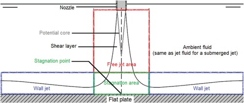
In heat transfer applications, impinging jets are a popular mechanism for cooling heated surfaces (Ortega-Casanova & Castillo-Sanchez, 2017) and frequent examples of their use are cooling electronic devices (Narumanchi et al., 2005), cooling in industrial machining processes (An et al., 2008), glass tempering (Sozbir & Yao, 2017; Yu et al., 2017), cooling of windshields of vehicles (Li et al., 2013) or when the temperature of irradiated targets must be reduced (Selvaraj et al., 2016), amongst many others. The complex nature of a turbulent impinging jet flow makes further work necessary to evaluate and predict the characteristics of heat transfer (Goldstein & Franchett, 1988; Shum-Kivan et al., 2014; Uddin et al., 2013). Initial research in this field dates back to 1951, with the experimental approach carried out by Friedman and Mueller (1951), and to 1953, when Kenzios combined theory and experiments in his doctoral thesis (Kezios, 1956). Since then, the jet flow is normally divided into three areas, the free jet area (which includes the potential core and shear layer), stagnation area and wall jet area respectively, as shown in Figure 1. Thus, an improvement of the cooling in the stagnation region and a radial distribution of the heat transfer along the wall jet region is generally desired.

Figure 1. Impinging jet zones. Adapted from O'Donovan and Murray (2007a).

Numerous authors have studied which parameters influence this heat transfer mechanism. As early as in Gardon and Akfirat (1966) analyzed the influence of the nozzle-to-plate distance, concluding that the maximum heat transfer in the stagnation region is reached at a separation of approximately six times the diameter. Also, the heat transfer within the potential core has been demonstrated to be essentially independent to the jet distancing, as reported by Hrycak (1983). When the jet is tilted, the heat transfer distribution is modified, being the point of maximum heat transfer (stagnation point) shifted towards the area of higher compression on the flat plate. Its value is increased if the inclination is decreased. The displacement is found to be sensitive to smaller separation of the jet to the plate (Goldstein & Franchett, 1988; Ichimiya & Nasu, 1993). To model turbulence in these configurations is complex, as most turbulence models are developed for parallel flow to the plate, as evidenced in Craft et al. (1993). The impinging jet considered in the present paper is turbulent. The existence of turbulence in wall jets is, in fact, recommendable since the radial Nusselt distribution strongly depends on this feature, as shown by several authors (Behnia et al., 1999; Granados-Ortiz et al., 2019; Uddin et al., 2013). These authors explicitly outlined the presence of secondary peaks in the Nusselt profile due to the transition to turbulent flow. They also pointed out the complexity in turbulence modeling of impinging jets, where even high-fidelity simulations such as Large Eddy Simulations (LES) may have difficulties to reproduce accurately experimental results (Granados-Ortiz et al., 2019; Uddin et al., 2013).

Swirling flows have been a hot-topic line of research for decades (Lucca-Negro & O'Doherty, 2001). Depending on the swirl mechanism, swirl intensity definition can be based on geometric or velocity considerations. For instance, the swirl number can be defined as the ratio of the azimuthal (or tangential) characteristic velocity to the axial characteristic velocity. Experimental studies have established that swirl has large scale favorable effects on various aspects of jet flows, such as spreading jet growth and instabilities, flow entrainment and decay (Gupta et al., 1984), leading to an increase of heat transfer because of rotation (Rose, 1962). Visualization techniques applied in Nuntadusit et al. (2012) showed that heat transfer rates of the moderate swirling jets ($S=0.4$) are found to enhance the non-swirling jet performance, whereas those of larger swirl numbers ($S=0.78$ and $0.94$) worsen the performance in comparison to the non-swirling jet. This is so due to flow momentum and velocity profiles of the jets, which are dependent on the device used for swirl generation (Granados-Ortiz et al., 2019). The most relevant phenomenon when dealing with swirling flows is recirculation bubble. At low swirl level ($S\lesssim 0.7$ Lucca-Negro & O'Doherty, 2001), certain level of radial or azimuthal pressure gradients may exist as a consequence of the centrifugal forces, but these do not create recirculation areas. When the swirl intensity is increased notably, a strong interaction between the axial and azimuthal velocity components is observed. In this situation, the adverse pressure gradient is notorious and a recirculation bubble appears, which is centered at the jet centerline.

1.1. Use of nanofluids in heat transfer with impinging jets

Regarding the working fluid, this can be also improved in order to increase heat transfer. Maxwell was the first to develop a theoretical model for the thermal conductivity of a suspension of spherical particles, estimating that the improvement of this property would be more pronounced with the increase of the volume fraction of particles and the relation between the area and the volume of the same (Levin & Miller, 1981). Hamilton and Crosser (Hamilton & Crosser, 1962) simplified the model, by providing correlations that made it possible to obtain the thermal conductivity of the working fluid according to the properties of the base materials, shape of the nanoparticles and concentration of the mixture. From this, other simpler models were developed, such as the one given by Wasp et al. (1977). However, the high concentration of the large-sized nanoparticles was an important drawback, leading to a lack of stability in the mixture suspension and wear (Wang & Mujumdar, 2007). In Choi and Eastman (1995) proposed that the particles should be of nanometric size. By applying the Hamilton and Crosser correlation, Choi obtained a significant improvement in heat transfer, reducing the power required by the heat exchanger pumps (Choi & Eastman, 1995). In this work, the term ‘nanofluids’ was introduced to refer to the new highly conductive refrigerant resulting from the addition of nanometric size particles in fluids such as water, ethylene glycol or oil, which revolutionized the concept proposed by Maxwell more than 100 years earlier. Although Choi's model was theoretical, Eastman's experimental results (Eastman et al., 1996) and Lee's ones (Lee et al., 1999) were in accordance with the theoretical predictions. Specifically, Eastman obtained a heat transfer improvement of $60\mathrm{\%}$ with a volume fraction of only $5\mathrm{\%}$. While these conclusions may seem promising, there are still open discussions on the general acceptance of the models developed in the literature. The different instrumentation used in each laboratory and the still poor theoretical knowledge on the fluid nanoparticle mechanics does not shed enough light on the lack of agreement between results (Keblinski et al.,2005).

Some papers argue that some of the open questions may be solved by analyzing the behaviour of nanofluids at a microscopic scale (Wang & Xu, 1999; Xuan & Roetzel, 2000). Brownian motion, thermal diffusion (Xuan & Li, 2000) or liquid-solid interface (Yu & Choi, 2003, 2004) have been taken into account, attributing to this layer the great change in thermal conductivity. Unfortunately, there is not yet a contrasted universal model to jointly account all these phenomena. Recent works in the literature are using advanced Artificial Intelligence techniques to characterize thermophysical properties of nanofluids. For instance, Sadeghzadeh et al. (2020) used Artificial Neural Networks (ANN) to predict the thermophysical properties of a ${\mathrm{T}\mathrm{i}\mathrm{O}}_2-{\mathrm{A}\mathrm{l}}_2{\mathrm{O}}_3$/water nanofluid, which was previously synthesized in the laboratory. In their work, relationships among concentration, temperature, thermal conductivity and viscosity were analyzed. An ANN predictor was also used in Ahmadi, Sadeghzadeh, et al. (2019) to estimate the dynamic viscosity of ${\mathrm{S}\mathrm{i}\mathrm{O}}_2$/ethylene glycol-water nanofluids on 160 experimental data from the literature. Although the method demonstrated high accuracy, the performance of the model could be improved by collecting more experimental data. In Nasirzadehroshenin et al. (2020) ANN are used again to model the heat transfer performance of carbon nanotube (CNT)/water nanofluid in a horizontal tube with a twisted tape. The experimental results were used to train the ANN to obtain correlations for the Nusselt number, friction factor and overall thermal performance of this heat exchanger. Ahmadi, Mohseni-Gharyehsafa, et al. (2019) utilized ANN, Multivariable Polynomial Regression (MPR) and Multivariable Adaptive Regression Splines (MARS) to characterize the dynamic viscosity dependence to the relevant parameters of a silver Ag-water nanofluid. As training data in their investigation, they used a series of experimental data available from the literature. In Baghban et al. (2019) an Adaptive Network-based Fuzzy Inference System (ANFIS) code was used to estimate the viscosity of nanofluids. Their work demonstrated that ANFIS is a very accurate tool in the estimation of the relative viscosity in nanofluids. A complex ANFIS and Least Square Support Vector Machine (LSSVM) method was succesfully tested in Razavi et al. (2019) to predict thermal conductivity of metal and metal oxide-based nanofluids with respect to input relevant parameters. However, the multi-phase model, which separately analyzes the solid particles and the fluid considering that each phase has a separate velocity vector and temperature field, seems to be gaining relevance (Peng et al., 2014). On the other hand, the lower complexity implicit in simulating a single-phase model, in which nanofluids are considered as homogeneous fluids, is the most used in computational research in the field, providing accurate results (Göktepe et al., 2014; Hussien et al., 2016).

To model nanofluids as a two-phase fluid is complex, since this approach must deal with continuity, momentum and energy equations associated to the particles and base fluid. As stated in Islami et al. (2013), when assuming that nanoparticles are ultra-fine ($<100$ nm) and that these are moving at the same velocity as the continuous liquid phase under local thermal equilibrium conditions, then the nanoparticle mixture can be considered to behave like a single-phase fluid. In Lotfi et al. (2010) the forced convective heat transfer of a ${\mathrm{A}\mathrm{l}}_2{\mathrm{O}}_3$-water nanofluid to the walls of a horizontal tube is studied by means of three models: single-phase, two-phase and mixture. In this work, the single and two-phase modeling yielded identical results, but the mixture model was found to be more accurate. In Saberi et al. (2013) the same study was conducted on a similar tube but vertical, and they concluded that the mixture model had better performance to model the convective heat transfer coefficient. Nonetheless, the single-phase model was more accurate to estimate the fluid mean bulk temperature. Throughout the study, the differences between the mixture and single-phase approach were not relevant. Moreover, the higher the Reynolds number, the closer to experimental data. Also Bianco et al. (2009) studied nanofluids for forced convection in a developing pipe flow by using different two-phase models to compare to single-phase performance. They found in the comparison that these results are similar, and the use of a single-phase flow is, in their own words, a ‘winning first glance approach in the study of new mixtures, considering also the low cost connected to it’, in reference to the few information required from the particles and base flow.

In terms of experimental works in the literature of impinging jets using nanofluids, there are several interesting works out there which evince the interest in the present investigation for engineering applications. For instance, in Tiara et al. (2016), a Cu–Al layered double hydroxide nanofluid at 120 ppm, along with different additives, was used together with the base fluid as an impinging jet in order to enhance the thermal properties of a steel plate (AISI 304) that was initially at 900${}^{\circ }$C. In Sorour et al. (2019), different experiments were conducted by using ${\mathrm{S}\mathrm{i}\mathrm{O}}_2$ nanofluid up to $8.5\mathrm{\%}$ solid volume fraction, and it was observed that the Nusselt number increased with the volume fraction and Reynolds number. Additionally, in Singh et al. (2016), the effect of different nanofluids (${\mathrm{T}\mathrm{i}\mathrm{O}}_2$, ${\mathrm{A}\mathrm{l}}_2{\mathrm{O}}_3$ and ${\mathrm{S}\mathrm{i}\mathrm{O}}_2$) and different concentrations are tested experimentally for a laminar single jet. This investigation concludes that they behave similarly at the same concentration, possibly because the same size of the particles, and also that the use of nanofluids enhances heat transfer in comparison to water jets. In Li et al. (2012) a $\mathrm{C}\mathrm{u}$-water nanofluid is tested experimentally and their results show a remarkable increase in the heat transfer coefficient of the base fluid when using nanofluids. Similarly, in Sun et al. (2016) $\mathrm{C}\mathrm{u}$ nanofluids are applied to heat transfer in a single impinging jet, by testing in this experimental work different jet angles, flow rates, nozzle shapes, nozzle-to-plate distances and concentration of nanoparticles. This study reports that the use of $\mathrm{C}\mathrm{u}$ nanofluids enhance heat transfer, especially for orthogonal jets, whereas pressure drop is not remarkably affected. In Mitra et al. (2012), ${\mathrm{T}\mathrm{i}\mathrm{O}}_2$-water and water-multiwalled carbon nanotubes (MWCNT-water) nanofluids are applied to the study their boiling heat transfer aspects by means of laminar jets. Again, it is observed that nanofluids enhance the cooling process. Moreover, it is reported that the vapor film stability may be affected by the presence of nanoparticles, which leads to a shift in the boiling curve of the regime. Additionally, in Wongcharee et al. (2017), swirling jets with $\mathrm{C}\mathrm{u}\mathrm{O}$ nanofluid are applied in experiments to increase heat transfer by impingement with different $\mathrm{C}\mathrm{u}\mathrm{O}$ concentrations. The Reynolds numbers considered ranged between 1600 and 9400, and the swirl is generated by means of twisted tapes. These experimental investigations encourage the objective of the present computational work, where the application of a swirling/non-swirling jet flow at high Reynolds number regime, with different ${\mathrm{A}\mathrm{l}}_2{\mathrm{O}}_3$ nanoparticle concentrations, swirl intensities and nozzle-to-plate distances is studied numerically to find an efficient cooling configuration.

Regarding the computational works in the literature of impinging jets using nanofluids, one of the most relevant aspects is the ability to model the behaviour of a nanofluid. As seen earlier in the discussion on the different approaches to simulate nanofluids in general CFD applications, these can be simulated by either a single-phase or a multi-phase approach. In impinging jets, the assumption of single-phase flow has been used the most in the literature in works of moderate/high Reynolds. A reason may be that, as explicitly stated in Kilic and Ali (2019), ‘it is determined that Brownian motion effect is more significant for low Reynolds number’. Also, makes sense that other effects such as sedimentation, thermophoresis or particle clustering are more unlikely to happen under the influence of strong convection and turbulence. Kilic and Ali (2019) used the single-phase approach to study the heat transfer with an array of three impinging jets and different types of nanofluid. They observed that by increasing the concentration from $\varphi =2\mathrm{\%}$ to $8\mathrm{\%}$ leads to an improvement of a $10\mathrm{\%}$ on area-weighted heat transfer. The work in Teamah et al. (2016) consists of both a numerical single-phase and experimental study on nanofluid jets impinging on a flat plate at different Reynolds numbers and concentrations, achieving almost identical results. In Paulraja et al. (2018) an impinging jet flow ranging between $Re=3000-\mathrm{10,000}$ on a surface with protusions is also simulated succesfully by means of a single-phase approach. Manca et al. (2011) simulated a confined slot impinging jet of a $Re=5000-\mathrm{20,000}$ and up to a $\varphi =6\mathrm{\%}$. Dutta et al. (2016) simulated both laminar ($Re=100-300$) and turbulent ($Re=10000-\mathrm{30,000}$) ${\mathrm{A}\mathrm{l}}_2{\mathrm{O}}_3$-water confined impinging jets for heat transfer, using the single-phase approach in both cases. In Selimefendigil and Öztop (2018) a low Reynolds number impinging jet of a nanofluid was used for cooling purposes of an isothermal heated surface with an adiabatic rotating cylinder. It was observed that both the rotation and the location of the cylinder affect the cooling of the heated surface. An original work in Ersayın and Selimefendigil (2013) was also carried out on heat transfer from a low Reynolds impinging jet to a moving plate, by studying different concentrations for the single-phase jet. The jet was also transformed into a pulsating jet (also known as synthetic jet) at different frequencies. Thus, most works in the literature used single-phase flows, achieving successful results with less computational efforts than a multi-phase approach.

The present investigation aims to study computationally a submerged impinging swirling/non-swirling turbulent jet flow for cooling processes using a ${\mathrm{A}\mathrm{l}}_2{\mathrm{O}}_3$-water nanofluid as working fluid. As one can observe by means of a quick literature review, the number of computational works in the literature on impinging jets using nanofluids is considerably lower than the amount of experimental works. The reason is attributed to two important facts. First, as stated in Granados-Ortiz et al. (2019), this imbalance between experimental-computational works is also observed in classic literature on heat transfer by impinging air or water jets. It was discussed earlier in this section that the modeling of turbulence in impinging jets is challenging (it is considered a case of complex flow because of the sudden changes in velocity magnitude and direction, the shear-layer interaction and the transition to turbulence (Granados-Ortiz & Ortega-Casanova, 2020)). Even LES simulations usually fail to model accurately such flow in heat transfer applications (Granados-Ortiz et al., 2019; Shum-Kivan et al., 2014). Second, as also stated earlier, to model nanofluids is not either easy because it requires the modeling of a complex two-phase flow. The continuity, momentum and energy equations involve both fluid and nanoparticles. Also, although high-speed flows are expected to present less drawbacks in nanofluid modeling as discussed previously, most computational works are related to laminar flows. There is an important dearth of literature on computational works of high-Reynolds impinging turbulent jet flows using nanofluids. Furthermore, there is no literature on CFD of impinging turbulent swirling jet flows with nanofluids. Thus, engineers who intend to develop designs with complex turbulent nanofluid flows do not have a decent amount of previous references for guidance beforehand. Computational tools are nowadays a central part of mechanical engineering design, so our work is motivated to fill this knowledge gap. Due to low-cost tools are valuable in industrial practice, the use of RANS and a single-phase approach is also attractive because of the strong savings in computational resources. It has been demonstrated in recent literature that the use of certain configurations of the $k-\omega$ turbulent model in RANS works excellent (even better than LES) in this type of impinging swirling jet (see, for instance, Granados-Ortiz & Ortega-Casanova, 2020 for details). Thus, the strong limitation in reproducing the secondary peak realistically for $H/D=2$ is overcome in the present research. In addition to the CFD analysis, for quick prediction in engineering practice, correlation models are given in this work to estimate the heat transfer at the stagnation point, area-averaged value and uniformity, for a wide range of swirl intensity, concentration of nanoparticles, and close and intermediate nozzle-to-plate distances.

The structure of the paper is as follows. In Section 2, the computational domain, together with the governing equations, boundary conditions, output parameters and thermophysical properties of the nanofluid are described. Next, in Section 3, some numerical considerations are given, such as the validation with experimental results and a grid convergence study. After this section, Section 4 is devoted to present and discuss all the results found. Finally, in Section 5 the conclusions are given.

2. Formulation of the problem

In the modeling of a symmetric circular swirling turbulent jet, which is impinging against a solid flat plate with diameter $8D$ (being D the diameter of the jet), azimuthal symmetry of the problem can be considered (axisymmetry). Thus, the simulations have been converged as 2D axisymmetric RANS using FLUENT. The axisymmetry of this type of jet has been analyzed by several researchers both computationally and experimentally. For instance, Panda and McLaughlin (1994) observed during their experiments an evident axisymmetry in swirling free jets at high Reynolds number. Similarly, Facciolo (2006) observed experimentally that axisymmetry too for turbulent jets at mid-high swirl intensity. He also studied such jets flows computationally. Other computational studies that considered the swirling jet as axisymmetric are (Granados-Ortiz et al., 2019; Herrada et al., 2009; Ortega-Casanova, 2012; Ortega-Casanova & Castillo-Sanchez, 2017; Owsenek et al., 1996; Shuja et al., 2003), which demonstrated high accuracy with two-dimensional models. A 2D section of the domain and boundary conditions, which is also the computational domain, can be seen in Figure 2. This depicts the impingement of the flow at a known distance H to the plate. The boundary conditions in ANSYS-Fluent (please see ANSYS, 2009 for further details on each boundary condition) depicted in Figure 2 are:

Figure 2. Sketch of the geometry and boundary conditions used in ANSYS-Fluent.

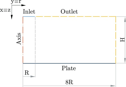
• Axis: Symmetry axis boundary condition (with zero flux of all quantities across the symmetry boundary).

• Inlet: The axial and azimuthal velocity profiles, together with their turbulence characteristics (Ahmed et al., 2015) are imposed onto the simulation as profile files (.prof) in ANSYS-FLUENT. The procedure that has been followed to input the turbulence profiles is described below.

• Pressure outlet: The pressure is imposed at the defined boundaries to the atmospheric pressure and transported quantities have gradients fixed to zero value.

• Wall (Plate): A fixed heat flux is applied and no-slip condition on it.

The flow is a nanofluid with constant density ${\rho }_{nf}$ and viscosity ${\mu }_{nf}$ (nf stands for nanofluid throughout the paper). Therefore, considering the axisymmetric, turbulent, steady, and incompressible jet flow, the motion of the fluid is governed by the continuity, momentum and energy equations, which using compact notation are: (1) $\begin{array}{rl}& \frac{\mathrm{\partial }{V}_i}{\mathrm{\partial }{x}_i}=0;\end{array}$(1) (2) $\begin{array}{rl}\frac{\mathrm{\partial }\left(V_i{V}_j\right)}{\mathrm{\partial }{x}_j}& =-\frac{1}{{\rho }_{nf}}\frac{\mathrm{\partial }P}{\mathrm{\partial }{x}_i}+\frac{{\nu }_{nf}}{{\rho }_{nf}}\frac{\mathrm{\partial }}{\mathrm{\partial }{x}_j}\left[\frac{\mathrm{\partial }{V}_i}{\mathrm{\partial }{x}_j}+\frac{\mathrm{\partial }{V}_j}{\mathrm{\partial }{x}_i}\right.\\ & -\left.\frac{2}{3}{\delta }_{ij}\frac{\mathrm{\partial }{V}_l}{\mathrm{\partial }{x}_l}\right]+\frac{\mathrm{\partial }\left(-\overline{v_i^{\prime }{v}_j^{\prime }}\right)}{\mathrm{\partial }{x}_j};\end{array}$(2) (3) $\begin{array}{rl}& \frac{\mathrm{\partial }}{\mathrm{\partial }{x}_i}\left[V_i(\rho e+P)\right]=\frac{\mathrm{\partial }}{\mathrm{\partial }{x}_j}\left[K_{eff}\frac{\mathrm{\partial }T}{\mathrm{\partial }{x}_j}\right],\end{array}$(3) where $V_i$ are the velocity components, with $i=z,r,\theta$ the axial, radial and azimuthal subscripts, whereas e is the internal energy per unit mass, T is the temperature and P is the pressure. Additionally, ${\delta }_{ij}$ is the Dirac's delta, $K_{nf}$ is the thermal conductivity, $K_{eff}=K_{nf}+K_t$ is the effective thermal conductivity and $K_t$ is the turbulent thermal conductivity $K_t=c_{p_{nf}}{\mu }_t/P{r}_t$. In the $K_t$ expression, $P{r}_t$ is the turbulent Prandtl number, ${\mu }_t$ is the turbulent dynamic viscosity, and the term $c_p$ is the fluid heat capacity. In ANSYS-Fluent© the default value of $P{r}_t$ is $P{r}_t=0.85$, which can be adjusted in the turbulent model if necessary. To solve the unknown velocity component fluctuations $v_i^{\prime }$, the problem must be closured by means of a turbulent model. In the present work, The Shear Stress Transport (SST) $k-\omega$ model is used, and the two closure equations the turbulent kinetic energy k and specific turbulent dissipation rate ω are: (4) $\begin{array}{rl}& {\rho }_{nf}\frac{\mathrm{\partial }}{\mathrm{\partial }{x}_i}\left(k{V}_i\right)=\frac{\mathrm{\partial }}{\mathrm{\partial }{x}_j}\left({\mathrm{\Gamma }}_k\frac{\mathrm{\partial }k}{\mathrm{\partial }{x}_j}\right)+G_k-Y_k,\end{array}$(4) (5) $\begin{array}{rl}& {\rho }_{nf}\frac{\mathrm{\partial }}{\mathrm{\partial }{x}_i}\left(\omega V_i\right)=\frac{\mathrm{\partial }}{\mathrm{\partial }{x}_j}\left({\mathrm{\Gamma }}_{\omega }\frac{\mathrm{\partial }\omega }{\mathrm{\partial }{x}_j}\right)+G_{\omega }-Y_{\omega },\end{array}$(5) where ${\mathrm{\Gamma }}_k$ and ${\mathrm{\Gamma }}_{\omega }$ are the effective diffusivity, $G_k$ and $G_{\omega }$ are the generation, and $Y_k$ and $Y_{\omega }$ are the dissipation of k and ω, for each term respectively. Further information on their definition and implementation can be found in ANSYS (2013).

For the sake of formality, Equations (1(1) $\begin{array}{rl}& \frac{\mathrm{\partial }{V}_i}{\mathrm{\partial }{x}_i}=0;\end{array}$(1) )–(5(5) $\begin{array}{rl}& {\rho }_{nf}\frac{\mathrm{\partial }}{\mathrm{\partial }{x}_i}\left(\omega V_i\right)=\frac{\mathrm{\partial }}{\mathrm{\partial }{x}_j}\left({\mathrm{\Gamma }}_{\omega }\frac{\mathrm{\partial }\omega }{\mathrm{\partial }{x}_j}\right)+G_{\omega }-Y_{\omega },\end{array}$(5) ) can be made dimensionless. The axial average velocity of the impinging jet $U_c$ is used as characteristic velocity, the diameter of the pipe D is used as characteristic length, and ${\rho }_{nf}{U}_c^2$ as characteristic pressure, with ${\rho }_{nf}$ being the density of the fluid, ${\mu }_{nf}$ its viscosity and ${\nu }_{nf}={\mu }_{nf}/{\rho }_{nf}$ its kinematic viscosity. The Reynolds number is thus defined as $Re=U_{c}D/{\nu }_{nf}$, which is kept constant throughout this work ($Re=\mathrm{35,000}$). The molecular Prandtl number is defined as $Pr=c_{p_{nf}}{\mu }_{nf}/K_{nf}$. As aforementioned, the fluid density and viscosity are considered constant since the flow is incompressible, but dependent on the concentration of nanoparticles. The dimensionless distance H from the plate to the nozzle has been fixed to $H/D=2$ and $H/D=4$.

According to Ahmed et al. (2015), the turbulent characteristics of the imposed jets are not constant at the nozzle exit (inlet of the computational domain). Thus, this property must be modeled as a profile inlet condition, as done for the inlet velocity profiles. To that end, from the known experimental velocity component fluctuations $v_i^{\prime }$, firstly the turbulence intensity $I$, and then $k$ and $\omega$ have been modeled. The turbulence intensity can be evaluated as (6) $I=\frac{V^{\mathrm{\prime }}}{U_c}$(6) where $V^{\mathrm{\prime }}$ is the root-mean-square of the velocity fluctuations computed as (7) $V^{\prime }=\sqrt{({v_r^{\prime }}^2+{v_z^{\prime }}^2+{v_{\theta }^{\prime }}^2)/3}.$(7) The radial profiles of the azimuthal and axial fluctuations are given in Ahmed et al. (2015), with the radial velocity component null. Once I is known, the turbulent kinetic energy can be evaluated as ANSYS (2009) and Sharma and Sharma (2017) (8) $k=\frac{3}{2}(I{U}_c{)}^2.$(8) Then, ω can be related to k by the expression (ANSYS, 2009; Sharma & Sharma, 2017) (9) $\omega =\frac{k^{1/2}}{C_{\mu }^{1/4}l},$(9) where $C_{\mu }$ is an empirical constant, typically of 0.09 value, and l is the turbulent length scale, which is defined by the approximation (ANSYS, 2009; Sharma & Sharma, 2017) (10) $l=0.07L,$(10) being L the characteristic length of the problem, i.e. the diameter of the jet D.

To quantify the efficacy of the cooling on the surface, the Nusselt number (ratio between heat transfer due to convective and conductive mechanics) is defined as (11) $Nu=\frac{h_{c}D}{K_{nf}},$(11) where $h_c$ is the convective heat transfer coefficient. Specially relevant is the Nusselt number at r = 0 (stagnation point) denoted by $N{u}_0$, and the area-weighted average value ($\overline{Nu}$), defined as (12) $\overline{Nu}=\frac{1}{A}{\int }_{A}Nu\mathrm{d}A=\frac{1}{A}\sum _{i=1}^{n}N{u}_i\left|A_i\right|,$(12) with $N{u}_i$ the Nusselt number at the ith element on the plate grid, $A_i$ the surface area of the ith element, and A the total surface area of an extension of $8D$.

The uniformity of the heat transfer is an important observation that defines the gradient of the cooling performance. To that end, the uniformity is evaluated by means of the standard deviation of the Nusselt number distribution: (13) $\sigma =\frac{\sqrt{\frac{1}{A}\left({\int }_A\sum _{i=1}^n\left(N{u}_i-\overline{Nu}\right)\mathrm{d}A\right)}}{\overline{Nu}}.$(13) Theoretically, if $Nu\left(r\right)\simeq \mathrm{c}\mathrm{o}\mathrm{n}\mathrm{s}\mathrm{t}\mathrm{a}\mathrm{n}\mathrm{t}$, $\sigma \simeq 0$. Thus, the lower the σ, the more uniform the cooling by forced convection. This is a relevant feature for the quality of certain cooling applications, such as tempering of glasses (Monnoyer & Lochegnies, 2008; Sozbir & Yao, 2017).

Since the flow is a swirling and non-swirling jet flow in this work, the swirl intensity must be formally quantified. This parameter is usually defined as the ratio between the azimuthal or tangential bulk velocity ($V_c$) over the axial bulk velocity: (14) $S=\frac{V_c}{U_c},$(14) with (15) $\begin{array}{rl}{V}_c& =\frac{2}{(D/2{)}^2}{\int }_0^{D/2}r{V}_{\theta }\mathrm{d}r\mathrm{a}\mathrm{n}\mathrm{d}\\ U_c& =\frac{2}{(D/2{)}^2}{\int }_0^{D/2}r{V}_z\mathrm{d}r,\end{array}$(15) being averaged velocities at the nozzle exit section (Ahmed et al., 2015).

To model the thermophysical properties of a nanofluid, with water as base fluid and aggregation of nanoparticles of ${\mathrm{A}\mathrm{l}}_2{\mathrm{O}}_3$ in the present application, a single-phase model can be used (Selimefendigil & Öztop, 2014). The single-phase model can be used under the assumption that the water and solid particles are moving at the same velocity and under thermal equilibrium. In this case, the effective density of the nanofluid can be modeled by the well-known two phase mixture model by the expression (16) ${\rho }_{nf}=(1-\varphi ){\rho }_{bf}+\varphi {\rho }_p,$(16) where ${\rho }_{bf}$ is the base fluid density (water), ϕ is the volume fraction of nanoparticles and ${\rho }_p$ is the density of the nanoparticles. Thus, the subscripts bf, nf and p stand for the base fluid (water), nanofluid (water+nanoparticles) and nanoparticles, respectively. Additionally, under the aforementioned thermal equilibrium conditions, the specific heat of nanofluid is given by (17) $C_{nf}=(1-\varphi )C_{bf}+\varphi C_p.$(17) Also, the the dynamic viscosity ${\mu }_{nf}$ is obtained by means of the least squares curve fitting correlation on experimental data given by Wang and Xu (1999): (18) ${\mu }_{nf}={\mu }_{bf}(123{\varphi }^2+7.3\varphi +1).$(18) Lastly, the thermal conductivity of the nanofluid $K_{nf}$ can calculated by means of the well-known Hamilton & Crosser model (Hamilton & Crosser, 1962): (19) $K_{nf}=K_{bf}(4.97{\varphi }^2+2.72\varphi +1).$(19) The thermophysical properties of both base fluid and nanoparticles are shown in Table 1.

Table 1. Thermophysical properties of the base fluid and nanoparticles.

Physical property	Water (bf)	${\mathrm{A}\mathrm{l}}_2{\mathrm{O}}_3$ (p)
C (J/kg-K)	4182	773
ρ (kg/m${}^3$)	$998,2$	3880
μ (Pa s)	$993\times {10}^{-6}$	–
K (W/m-K)	$\mathrm{0,597}$	36

Finally, according to all these thermophysical properties, the Prandtl number of the nanofluid flow can be evaluated as (20) $\begin{array}{rl}P{r}_{nf}& =\frac{C_{nf}{\mu }_{nf}}{K_{nf}}\\ & =\frac{\left[{\mu }_{bf}(123{\varphi }^2+7.3\varphi +1)\right]\left[(1-\varphi )C_{bf}+\varphi C_p)\right]}{K_{bf}(4.97{\varphi }^2+2.72\varphi +1)},\end{array}$(20) which can be simplified to the expression (21) $P{r}_{nf}=P{r}_{bf}\frac{(123{\varphi }^2+7.3\varphi +1)\left(\right(1-\varphi )+\varphi \text{β})}{4.97{\varphi }^2+2.72\varphi +1},$(21) where β is the specific heat ratio, i.e. $\text{β}=C_p/C_{bf}\simeq 0.185$, and $P{r}_{bf}$ is the base fluid Prandtl number, i.e. $P{r}_{bf}=C_{nf}{\mu }_{nf}/K_{nf}\simeq 7$. Thus, when $\varphi \in [0,10]\mathrm{\%}$, then $P{r}_{nf}\in [7,14.4]$.

3. Numerical considerations

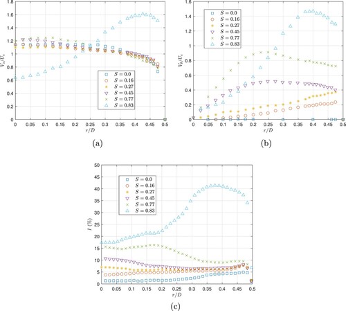
Regarding the boundary conditions (see Figure 2), the jet is modeled as a velocity-inlet condition, whose turbulence intensity, axial and azimuthal velocity components are those obtained experimentally in Ahmed et al. (2015). An example of the profiles is depicted in Figure 3. For different values of the volume fraction, the thermophysical fluid properties vary. Thus the characteristic velocity $U_c$ is varied too, in order to maintain the same Reynolds number throughout the study: $Re=\mathrm{35,000}$. For a full description of the boundary conditions, the symmetry axis is located at the left-hand side of the domain to coincide with the nozzle centerline, and the plate is located at the bottom. The plate is modeled as a non-slip heated wall condition, with an imposed heat flux of any known constant value. Since the dimensionless Nusselt number is the quantity of interest, the value of the heat flux is irrelevant. The boundary at the right-hand side and the upper boundary from the edge of the nozzle till the end of the plate are pressure-outlet at atmospheric pressure (see Figure 2).

Figure 3. Axial and azimuthal velocity dimensionless profiles, and turbulence intensity profiles imposed onto the inlet boundary for $\varphi =0\mathrm{\%}$ (water) and different swirl intensities S, according to Ahmed et al. (2015). (a) Axial velocity. (b) Azimuthal velocity and (c) Turbulence intensity.

The computational study is performed for an incompressible flow, for which a pressure-based formulation is applied. The SIMPLE algorithm (Semi-Implicit Method for Pressure-Linked Equations) is used for the pressure-velocity coupling (Patankar & Spalding, 1983), which employs a Predictor-Corrector approach. Due to the spatial discretization, cell values of the discretized scalar quantities are stored in the center of each cell in ANSYS-FLUENT (ANSYS, 2009). For the convective terms, the cell-center values must be interpolated at the cell faces by means of an upwind scheme. In the present work, Second Order Upwind schemes are used, which predict cell-face values by means of a Taylor series expansion. To construct the gradients, which are necessary not only for cell-face values estimation but also for velocity derivatives, a Least Squares Cell-based Algorithm is used.

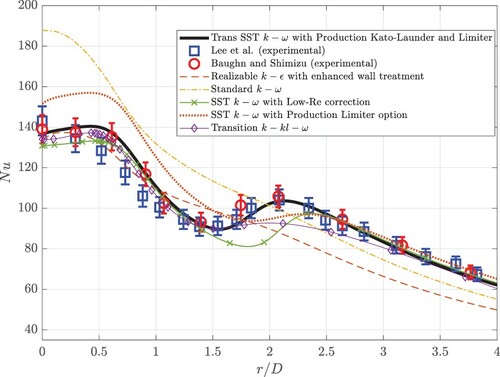
The turbulent model used in the CFD simulation of the impinging jet flow is the Transition SST $k-\omega$, which has been previously used with satisfactory results by several authors in impinging swirling/non-swirling jet flows for heat transfer, see e.g. Ortega-Casanova and Granados-Ortiz (2014), Ahmed et al. (2017), Granados-Ortiz et al. (2019), Ortega-Casanova and Castillo-Sanchez (2017), and Ortega-Casanova (2012), among others. In addition, it has been conducted a validation test by comparing the Nusselt profile distribution provided by our simulation with data from Hee et al. (2002), and Baughn and Shimizu (1989). Specifically, the simulated performance for that purpose is a non-swirling ($S=0$) air jet with $Re=\mathrm{23,000}$ and impinging against the heated plate located at $H/D=2$. The comparison depicted in Figure 4 shows that the present work agrees quite well with data reported by previous authors, including the location and intensity of the secondary peak. This permits to validate both the turbulent modeling and the numerical considerations used in this study.

Figure 4. Validation of the CFD model for $Re=\mathrm{23,000}$ and $H/D=2$. Present work (Transition SST $k-\omega$ with Production Kato-Launder and Production Limiter) and other tested RANS turbulence models (see ANSYS, 2009 for details) compared to experimental data from Hee et al. (2002), and Baughn and Shimizu (1989) (5% error bars are also included).

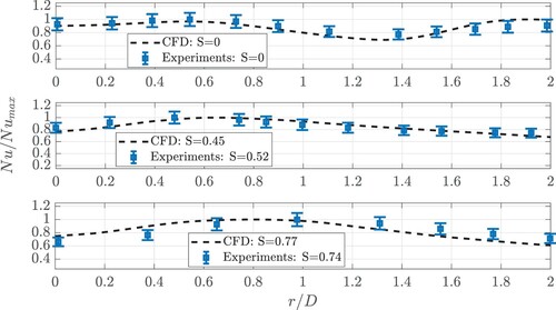
For the sake of rigor, a second validation has been carried out for $Re=\mathrm{35,000}$ and different values of S, since the numerical results provided in the next sections are under this Reynolds number regime and swirl intensities. The comparison is shown in Figure 5, where one can see that the current numerical results match very accurately with experimental data provided in Ahmed et al. (2016), for the normalized radial profile of the Nusselt number. Must be noted that there is a small discrepancy between the values of S in the reported profiles in Ahmed et al. (2015) and the values of S in the experiments in Ahmed et al. (2016), which may explain the small differences in the validation. By means of this validation is shown that the CFD simulation models accurately the thermal reality of the problem, being even able to reproduce the secondary peak of the Nusselt number for $S=0$.

Figure 5. Validation of the CFD model for $Re=\mathrm{35,000}$ and $H/D=2$ with different values of S. The inlet profiles are obtained from Ahmed et al. (2015), and experimental data was collected by the same authors in Ahmed et al. (2016).

In this section a discretization error analysis is also carried out. For this purpose, the CFD problem has been solved using four different structured rectangular grids, with increasing number of cells, so that one can study how a quantity of interest varies along with the amount of cells. When to further refine the mesh has no variation in the quantity of interest, grid convergence is assumed. Actually, a reliable reference value for comparison is obtained by Richardson's Extrapolation (which would be the value for infinite cells). Thus, to quantify the discretization error, the Grid Convergence Index (hereinafter GCI), is computed following the methodology proposed by Roache (1994). In our study, the representative parameter is $N_{total}$ (total number of cells), and the refinement ratio can be defined as $r=N_i/N_{i+1}$ (with $N_i$ the number of cells of each mesh), which is kept almost constant. The second-order numerical methods used in this study imply a formal accuracy of $p_f=2$, whereas the observed accuracy is $p_o=6.28$, using the area-weighted average Nusselt number as quantity of interest (see Equation (12(12) $\overline{Nu}=\frac{1}{A}{\int }_{A}Nu\mathrm{d}A=\frac{1}{A}\sum _{i=1}^{n}N{u}_i\left|A_i\right|,$(12) )). This shows that the accuracy obtained in this study is actually greater than the one expected for the second order discretization schemes employed. The GCI results are presented both in Table 2 and in Figure 6, where one can see that the coarse mesh (with around 120 thousand cells) is the optimal one since the GCI${}_{4,3}$ is small enough to consider the results of high reliability.

Figure 6. Grid convergence study.

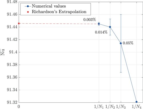
Table 2. Grid convergence study results.

i	Grid	$N_z$	$N_{total}$	$r_i$	$\overline{Nu}$	CGI${}_{i+1,i}$
1	Fine	651	$\mathrm{195,951}$	$\approx 1.3$	91.445	$0.003\mathrm{\%}$
2	Medium	501	$\mathrm{150,801}$	$\approx 1.3$	91.440	$0.014\mathrm{\%}$
3	Coarse	401	$\mathrm{120,701}$	$\approx 1.3$	91.414	$0.05\mathrm{\%}$
4	Very coarse	301	$\mathrm{90,601}$	–	91.321	–

It is relevant to point out from the mesh quality side that, in each mesh above considered, the distance of the first cell next to the flat plate wall is such that $y^{+}$ parameter remains approximately equals to unity. This permits to resolve the boundary layer and the heat exchange between the flat plate and the jet flow. The chosen $H/D=2$ mesh of $[N_r\times N_z]=[301\times 401]$ cells is depicted in Figure 7, where the full mesh and a zoom in on the near wall region is shown. The mesh for $H/D=4$ keeps the same nodal distribution for the boundary layer but the number of nodes in $N_z$ is increased: $[N_r\times N_z]=[301\times 601]$ cells.

Figure 7. Mesh for $H/D=2$. From left to right: Full mesh, zoom in of the mesh adjusted to the nozzle-to-plate height and zoom in on the near wall region. The red squares represent the region for which its zoom in is shown next. The green line is the inlet and the black line is the plate.

Finally, as discussed in the introduction section, the nanofluid can be simulated by either a single-phase or a multi-phase approach. The assumption of single-phase for impinging jets of nanofluids has been used the most in the literature in works of moderate/high Reynolds. Although all the aforementioned works used a single-phase approach, a comparison of results with the single-phase and multi-phase approach for the present investigation was developed as shown in Figure 8. This comparison has been carried out for two reasons: first, it was intended to analyze the present problem from all available numerical viewpoints. Second, there is an important dearth of literature regarding comparison of single and multi-phase modeling of impinging jets with nanofluids, which sometimes obscures the reliability on reported results.

Figure 8. Comparison between single-phase (SP) and multi-phase (Mixture and multi-phase Eulerian, MPE) simulations for $\varphi =2\mathrm{\%}$, $H/D=2$ and S = 0. PKL stands for Production Kato-Launder, and PKKL stands for both Production Kato-Launder and Production Limiter. Base fluid without nanoparticles ($\varphi =0\mathrm{\%}$) is included as reference in red solid line with circular markers. The radial distribution of Nusselt number, wall shear stress, turbulent kinetic energy and static pressure correspond to their values on the plate. The axial velocity profile is obtained from the jet centerline. (a) Nusselt. (b) Wall shear stress. (c) Turbulent kinetic energy. (d) Static pressure and (e) Axial velocity.

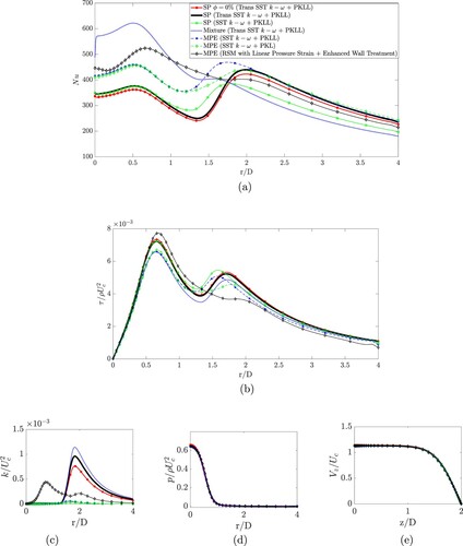
Many turbulence model combinations have been tested. In Figure 8 are shown the best results by single-phase (SP), mixture and multi-phase Eulerian (MPE) simulations for $\varphi =2\mathrm{\%}$ at $H/D=2$ and S = 0. Data for $\varphi =0\mathrm{\%}$ (water-only) is also included as reference, since results should not vary notably with a $2\mathrm{\%}$ in concentration of nanoparticles, as reported in all consulted experimental and numerical literature. Moreover, the use of a $\varphi =0\mathrm{\%}$ flow in the simulation was validated in Figure 5. Unfortunately, the Transition SST $k-\omega$ model, which performed the best in the validation studies, is not available in the MPE modeling in ANSYS-FLUENT. For this reason, the SST $k-\omega$ was tested. It can be observed in Figure 5 that this model performed different to the Transition one even in SP modeling. Thus, this is a drawback for MPE in ANSYS-FLUENT. The MPE results shown overpredicted the Nusselt distribution before the secondary peak, see Figure 8(a), but predicted accurately the position and magnitude of the secondary peak and heat transfer downstream. The overprediction is enough argument to discard the MPE modeling, since the SP performed more realistic. The mixture approach, although included the Transition $k-\omega$ turbulence model, provided a huge overprediction of the Nusselt number in the stagnation area and did not reproduce the secondary peak of the Nusselt number. However, this modeling yielded similar values of the turbulent kinetic energy on the plate to those reported with SP modeling, see Figure 8(c). The wall shear stress on the plate was similar for all the tested models, see Figure 8(b). In terms of static pressure and velocity fields, see Figure 8(d,e), respectively, the flow field with SP, mixture and MP was the same, with negligible differences.

To provide these results may help other researchers to figure out which modeling may or may not work. For instance, we do not recommend at all to use any model from the $k-ϵ$ turbulence model family in multi-phase modeling of this type of high-speed nanofluid jet. Their results deviated excessively from the expected performance. Amongst all the possibilities tested for Eulerian multi-phase modeling (Standard $k-ϵ$, RNG $k-ϵ$ and Realizable $k-ϵ$, all with different near wall treatments), none of these provided realistic heat transfer distributions on the plate. Concretely, the RNG $k-ϵ$ performance was totally unrealistic. The more sofisticated RSM turbulence model (Reynolds Stress Model) was also tested, despite other researchers in the literature showed that it is not a good option even for water/air-only impinging jets (Zuckerman & Lior, 2007). In Figure 8 can be seen that the trend of the Nusselt distribution for RSM with Linear Pressure Strain modeling is incorrect before the secondary peak. RSM with Quadratic Pressure Strain modeling was also tried, but the simulation did not converge.

Due to the single-phase approach is much less time consuming and provided more accurate results thanks to the availability in ANSYS-FLUENT of the Transitional SST $k-\omega$ turbulence model, in this work all the simulations are developed as single-phase model. One can also conclude that, from a thermal viewpoint, the SP performed the best. From a mechanical viewpoint, all modeling approaches provided similar results.

4. Results

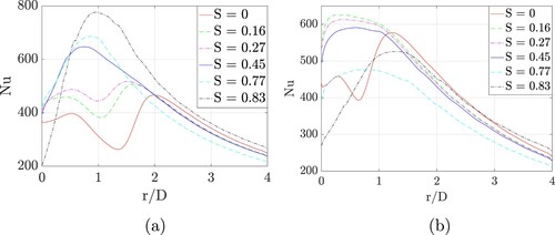
The aim of this section is to investigate and discuss the results of the cooling process by forced convection, quantified by means of the area-weighted averaged ($\overline{Nu}$) and stagnation ($N{u}_0$) Nusselt number, as well as its standard deviation (σ) in order to quantify the uniformity of the transfer. To that end, it has been simulated the impinging jet with six different volume fractions of nanoparticles, three swirl numbers and two nozzle-to-plate distances. A summary of the obtained results for the three above mentioned output parameters is shown in Figure 9.

Figure 9. Heat transfer results. Solid and dashed lines represent quadratic fitting of the numerical data. (a) $\overline{Nu}$ results. (b) $N{u}_0$ results and (c) σ results.

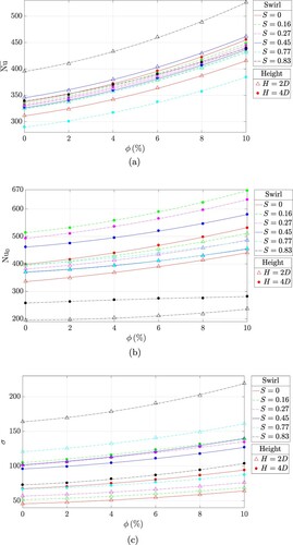
At the smallest nozzle-to-plate distance, $H/D=2$, the area-weighted averaged Nusselt number ($\overline{Nu}$) increases as the swirl intensity is increased, except for $S=0.77$, for which a decay is observed (see Figure 9(a)). This can be observed more clearly in Figure 10, where for instance $\varphi =8\mathrm{\%}$ is shown since all ϕ behave similarly. The increase of $\overline{Nu}$ as S is increased is due to the fact that the swirl enhances turbulence and mixing, as explained in Ahmed et al. (2017). This effect is found in the present simulations as shown in the turbulence intensity contours in Figure 11 (left column is $H/D=2$). One can see that $\overline{Nu}$ increases as swirl increases, but for $S=0.77$ it can be observed that the distribution of turbulence intensity on the plate is weak. This explains the decrease, since the largest values of the turbulence intensity are now only located in the shear layer and potential core. In Figures 9 and 10, a sudden change in trend is observed for $S=0.83$. This is because for such large swirl intensity a recirculation bubble appears, which changes the behaviour of the heat transfer (see Figures 12 and 13). This affects especially the $N{u}_0$, as will be discussed later. On the contrary, for $H/D=4$, $\overline{Nu}$ values are lower than for the short nozzle-to-plate distance when $S>0.27$. However, its value is greater when $S\le 0.27$. This may be because the large separation allows the jet spreading angle to increase (the stagnation area is smaller for $H/D=4$, see Figure 12, and the secondary peak in the Nusselt occurs at earlier r/D distance) and thus the heat transfer, as seen in contours levels of Figure 11(a,b). When the swirl number is increased, our results agree with those reported in Ahmed et al. (2017), where a transition is observed at $S=0.45$. The experimental approach described in Nuntadusit et al. (2012) led to equivalent results. In Ahmed et al. (2017) this feature is attributed to the more evident jet flow widening when impinging from a higher distance. This increase in the spreading angle is sensitive to the swirl generator used in Ahmed et al. (2017), as also pointed out in Granados-Ortiz et al. (2019).

Figure 10. Output parameters with respect to S for the indicated nozzle-to-plate distances and $\varphi =8$%.

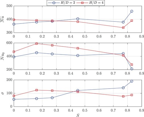
Figure 11. Turbulence intensity contours for $\varphi =8\mathrm{\%}$. (a) $S=0;H/D=2$. (b) $S=0;H/D=4$. (c) $S=0.16;H/D=2$. (d) $S=0.16;H/D=4$. (e) $S=0.45;H/D=2$. (f) $S=0.45;H/D=4$. (g) $S=0.77;H/D=2$. (h) $S=0.77;H/D=4$.

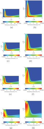
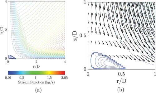
Figure 12. Dimensionless velocity magnitude contours for $\varphi =8\mathrm{\%}$. (a) $S=0;H/D=2$. (b) $S=0;H/D=4$. (c) $S=0.16;H/D=2$. (d) $S=0.16;H/D=4$. (e) $S=0.45;H/D=2$. (f) $S=0.45;H/D=4$. (g) $S=0.77;H/D=2$. (h) $S=0.77;H/D=4$.

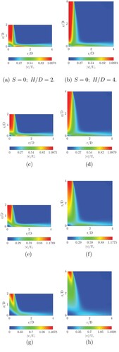
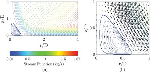
Figure 13. Streamlines for S = 0.83, $\varphi =8\mathrm{\%}$ and $H/D=2$. (a) Entire domain and (b) Detailed view of the recirculation bubble with velocity vectors.

Regarding the Nusselt number at the stagnation point, Figure 9(b) illustrates different trends. Regardless the nozzle-to-plate separation, it decreases as the swirl number increases in the range $0.16\le S\le 0.45$. This is because centrifugal forces spread the jet radially, thus preventing it from impinging directly on the center of the plate and reducing the heat transfer on that area. However, there is a improvement in $N{u}_0$ from non-swirling to swirling jet. Velocity magnitude contours depicted in Figure 12 illustrate this phenomenon, showing that the low velocity region around the stagnation point grows radially outwards as the swirl number increases, but can be observed that from $S=0$ up to $S=0.45$ the size of the stagnation region is reduced. Also, it can be seen in Figure 11 that from $S=0.45$ up to $S=0.77$ the turbulence intensity is increased in the stagnation region, thus compensating the radial growth of the stagnation region which would eventually decrease $N{u}_0$ for $H/D=2$. For $H/D=4$ such turbulence intensity is not enough, and $N{u}_0$ is decreasing even for $S=0.77$. In general terms, $N{u}_0$ increases as the nozzle-to-plate distance increases. In Figure 12 one can also see that the low velocity stagnation region becomes smaller when the jet impinges from a higher distance, as discussed in the analysis of $\overline{Nu}$. In addition, when the swirl intensity reaches $S=0.83$ and regardless the nozzle-to-plate separation, a recirculation bubble occurs (see Figure 12(e,f), which is also plotted in solid line in Figures 13 and 14, for $H/D=2$ and $H/D=4$, respectively. Streamlines outside the bubble-like are plotted in dashed line. As discussed by other authors (Ahmed et al., 2017), the heat transfer in the center of the plate is strongly diminished as a consequence of this bubble. According to Abrantes and Azevedo (2006), this is due to the low velocity at which this recirculation occurs. The bubble becomes, surprisingly, smaller for greater $H/D$ values, which achieve higher values of $N{u}_0$. This agrees with results reported by Ahmed et al. (2017).

Figure 14. Streamlines for S = 0.83, $\varphi =8\mathrm{\%}$ and $H/D=4$. (a) Entire domain and (b) Detailed view of the circulation bubble with velocity vectors.

The uniformity of the heat transfer, defined as the standard deviation of the Nusselt number distribution, is illustrated in Figures 9(c) and 10. The higher the standard deviation, the less uniform the heat transfer. The uniformity and the area-weighted averaged Nusselt number behave very similar, mainly because both parameters relate to the surface distribution of the Nusselt. Thus, the explanations presented in the discussion of $\overline{Nu}$ are also valid for σ. According to Figure 9(c), the addition of nanoparticles yields a less uniform heat transfer (σ increases). At short nozzle-to-plate distance, the increase of swirl intensity worsens the heat exchange, because of the aforementioned lower values of $N{u}_0$ and the fading of the secondary peak (see Figure 15). This result is directly related to the existence of two peaks for non-swirling/weakly swirling jet and a single peak for swirling flows in Figure 15. The secondary peak in Nusselt profiles has been observed by many authors (Abrantes & Azevedo, 2006; Ahmed et al., 2017; Granados-Ortiz et al., 2019; Ortega-Casanova & Castillo-Sanchez, 2017; Uddin et al., 2013) but there is not yet a clear universal accepted explanation. Some authors (Ahmed et al., 2017; O'Donovan & Murray, 2007b) attribute this to the increase in turbulence intensity. Specifically, in O'Donovan and Murray (2007a), Ashforth-Frost et al. (1997), Uddin et al. (2013), and Granados-Ortiz et al. (2019) it is pointed out that the secondary peak is consequence of the turbulence transition in the boundary layer development of the wall jet. At short nozzle-to-plate distance, when S is increased, the peak is shifted radially and progressively transformed into a single larger peak, so the the standard deviation increases. Generally speaking, for high separations, the potential core has more space to grow, which may be linked to the fast disappearance of the secondary peak when swirl is applied. This leads to a sudden increase in σ from $S=0$ to $S=0.16$, as a single large peak appears. For $S>0.16$, the large peak in heat transfer moves till the stagnation region (decreasing as S increases), thus decreasing σ. In the present problem under study, for $H/D=4$ and $S=0$ the secondary peak still appears so, as suggested in Ashforth-Frost et al. (1997), it may be because at this distance the plate remains in the area of influence of the potential core. For both H/D, the recirculation bubble also influences the uniformity of the Nusselt profiles. In Ianiro and Cardone (2012) it is remarked that uniformity fades away when the bubble appears, which agrees with results shown in Figure 9(c), where σ shows a sudden increase for $S=0.83$.

Figure 15. Nusselt profiles on the plate for different nozzle-to-plate distances and swirl intensities, but only one volume fraction, $\varphi =4$%. (a) $H/D=2$ and (b) $H/D=4$.

4.1. Correlation models

An additional objective in this paper is to provide correlations for heat transfer predictions (Ortega-Casanova, 2012). The proposed correlations relate, for each nozzle-to-plate distance $H/D$, the magnitudes of interest with the swirl intensity $S$ and the Prandtl number of the nanofluid (which depends on the considered volume fraction of nanoparticles ϕ). These models have the same terms for each $H/D$ value, but different values for the fitting coefficients. The correlation models have the form: (22) $\mathcal{F}={\text{β}}_1+{\text{β}}_2\cdot S+{\text{β}}_3\cdot P{r}_{nf}+{\text{β}}_4\cdot S^2+{\text{β}}_5\cdot S^3,$(22) where $\mathcal{F}$ can be any of the output parameters of interest, i.e. $\overline{Nu}$, $N{u}_0$ or σ; whereas ${\text{β}}_i$ are fitting constants. As can be seen, Equation (22(22) $\mathcal{F}={\text{β}}_1+{\text{β}}_2\cdot S+{\text{β}}_3\cdot P{r}_{nf}+{\text{β}}_4\cdot S^2+{\text{β}}_5\cdot S^3,$(22) ) is a third-order correlation in terms of S and linear order in term of $P{r}_{nf}$. This is so because the quantities of interest vary in a linear fashion when the concentration is varied. Additionally, due to the severe recirculation bubble appearing at $S=0.83$, which does not appear for $S\le 0.77$, values of $S>0.77$ are not considered in the correlation modeling. The appeareance of recirculation bubbles at larger swirl intensities makes not suitable to generalize the correlation models to large $S$ values.

All the fitting constants are shown in Table 3, where the mean relative error and the goodness of the fitting, in terms of $R^2$ and adjusted $R^2$ (denoted as $R_{adjusted}^2$), are included. The correlation for $\overline{Nu}$ does not need a third-order term for $S$. The parameter $N{u}_0$ could be also approximated by a correlation with second-order $S$ terms, but the $R^2$ measures would be around 0.75 for $H/D=2$, and 0.87 for $H/D=4$. The range of validity of the input parameters is $S\in [0,0.77]$ and $P{r}_{nf}\in [7,\sim 14]$. As aforementioned, the fitting constants ${\text{β}}_i$ of Equation (22(22) $\mathcal{F}={\text{β}}_1+{\text{β}}_2\cdot S+{\text{β}}_3\cdot P{r}_{nf}+{\text{β}}_4\cdot S^2+{\text{β}}_5\cdot S^3,$(22) ) have a specific value depending on the quantity of interest and the $H/D$ value, as can be seen in Table 3. The relative error between the numerical values and correlation values is calculated by (23) $error\left[\mathrm{\%}\right]=\frac{1}{N}\sum _{i=1}^N\left(\frac{\mid nu{m}_i-cor{r}_i\mid }{nu{m}_i}\right)\cdot 100,$(23) where N is the number of training points, $nu{m}_i$ is the ith numerical value and $cor{r}_i$ is the ith value predicted by the correlation. Figure 16 illustrates the goodness of each fit by plotting the 10% error bands. Moreover, a comparison between the numerical values and those predicted by Equation (22(22) $\mathcal{F}={\text{β}}_1+{\text{β}}_2\cdot S+{\text{β}}_3\cdot P{r}_{nf}+{\text{β}}_4\cdot S^2+{\text{β}}_5\cdot S^3,$(22) ) is shown in the figure for each output quantity of interest. It can be seen that, most predictions lie within the error bands. This, together with the error and the $R^2$ parameters as goodnesses of fit in Table 3, show that the proposed correlations are accurate, especially for $N{u}_0$ and $\overline{Nu}$.

Figure 16. Confrontation between numerical results and correlation values for (a) $\overline{Nu}$, (b) $N{u}_0$ and (c) σ.

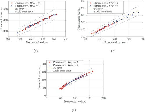
Table 3. Fitting constant values for the correlations depending on H/D values.

		Fitting constants
H/D	$\mathcal{F}$	${\text{β}}_1$	${\text{β}}_2$	${\text{β}}_3$	${\text{β}}_4$	${\text{β}}_5$	$R^2$	$R_{adjusted}^2$	error[%]
2	$\overline{Nu}$	206.43	154.31	14.53	168.58	–	0.9865	0.9849	1.01
	$N{u}_0$	249.60	635.40	13.26	−2130	1806	0.9726	0.9682	1.31
	σ	18.864	−162.87	3.55	1103.30	−975.19	0.9767	0.9730	6.25
4	$\overline{Nu}$	238.06	16.33	14.65	−114.88	–	0.9925	0.9916	0.85
	$N{u}_0$	289.80	1138	16.85	−3328	2284	0.9749	0.9708	1.92
	σ	39.93	367.61	3.94	−955.28	611.17	0.9742	0.9701	2.72

5. Conclusions

In the present study the cooling of surfaces by the application of a submerged turbulent swirling/non-swirling impinging jet of nanofluids has been studied numerically. To overcome successfully the difficulties in modeling of turbulent impinging jets and nanofluidic, the Transition SST $k-\omega$ turbulence model with the Production Kato-Launder and Production Limiter option with a single-phase approach have been used for numerical modeling in ANSYS-FLUENT. Concretely, the secondary peaks in the radial Nusselt number distribution for low swirl intensity have been reproduced with high accuracy, which is a very frequent issue in the literature. In this cooling process, the volume fraction of nanoparticles, the swirl intensity and the nozzle-to-plate distance have been varied in order to analyze the influence of these parameters on the applied heat transfer system performance, quantified by the area-weighted average value, the stagnation point value and uniformity of the Nusselt number on the flat plate.

The results from the computational analysis suggest that:

• In general terms, to add swirl is beneficial for the heat transfer at the stagnation point, except when a recirculation bubble appears at large $S$ or $S=0.45$ is exceeded at $H/D=4$. For $H/D=2$, the heat transfer at the stagnation point is worsened with increasing swirl number in the range $0.16<S<0.45$, due to the decrease of the size of the stagnation region and lower turbulence intensity. For $H/D=4$, this decrease occurs for $S>0.16$. A large nozzle-to-plate distance enhances the heat transfer at the stagnation region.

• For high swirl intensity jets the decrease in the heat transfer at the stagnation point is very noticeable as a consequence of the appeareance of a recirculation bubble.

• The surface averaged cooling process increases with increasing swirl number at $H/D=2$, only by increasing $S$ up to $S=0.45$. Then, it decreases for $S=0.77$ because of a reduction in turbulence intensity on the plate. When $S$ is further increased, the surface averaged heat transfer is again increased due to the appearance of a recirculation bubble. At $H/D=4$ distance, the surface averaged heat transfer decreases with increasing the swirl number, until the recirculation bubble appears.

• Regarding the uniformity of the surface cooling, at $H/D=2$ it decreases with increasing swirl intensity, and this is strongly related to the presence of peaks in the Nusselt profile. At $H/D=4$, for swirling jet flows uniformity is improved with increasing $S$, until the recirculation bubble appears.

• The increase in the fraction of nanoparticles enhances heat transfer at stagnation point and in average in all the tested configurations. It also decreases uniformity.

In addition to the conclusions above, from an optimization perspective:

• The maximum averaged heat transfer was observed for $S=0.83$ and $H/D=2$, whereas the maximum value at the stagnation point takes place for $S=0.16$ and $H/D=4$.

• The maximum level of uniformity (lowest σ) was reached at $S=0$ and $H/D=2$.

• Additionally, all the maximum values of $\overline{Nu}$, $N{u}_0$ and σ are obtained for the highest volume fraction of nanoparticles considered in the simulations, $\varphi =10\mathrm{\%}$.

Moreover, different correlation models have been proposed to predict the three quantities of interest, i.e. $\overline{Nu}$, $N{u}_0$ and σ, as function of the three input parameters, i.e. $S$, $H/D$ and ϕ (by means of $P{r}_{nf}$).

The use of nanofluids for such computational applications is still a field under developments to overcome some limitations, such as difficulties in modeling of the effect of turbulence on the secondary peak for the Nusselt number, the lack of universal models for the thermophysical properties and particle motion at microscale, or the lack of consensus in the performance of single-phase and multi-phase modeling. In addition, experimental analysis including low and high Reynolds numbers for the different swirl intensities would be of interest, since this would help to understand the impact of turbulence on this swirling nanofluid jet. Future work on using higher swirl intensities for the swirling jet flow analyzed in this paper is also encouraged, as the appearance of the circulation bubble leads to a different design performance.

Disclosure statement

No potential conflict of interest was reported by the author(s).

Additional information

Funding

The first and third author want to acknowledge the financial support from the UMA18-FEDERJA-184 grant.

References

- Abrantes, J. K., & Azevedo, L. F. A. (2006). Fluid flow and heat transfer characteristics of a swirl jet impinging on a flat plate. International Heat Transfer Conference 13. Begel House Inc.
- Ahmadi, M. H., Mohseni-Gharyehsafa, B., Farzaneh-Gord, M., Jilte, R. D., Kumar, R., & Chau, K.-w. (2019). Applicability of connectionist methods to predict dynamic viscosity of silver/water nanofluid by using ANN-MLP, MARS and MPR algorithms. Engineering Applications of Computational Fluid Mechanics, 13(1), 220–228. https://doi.org/https://doi.org/10.1080/19942060.2019.1571442
- Ahmadi, M. H., Sadeghzadeh, M., Maddah, H., Solouk, A., Kumar, R., & Chau, K.-w. (2019). Precise smart model for estimating dynamic viscosity of SiO 2/ethylene glycol–water nanofluid. Engineering Applications of Computational Fluid Mechanics, 13(1), 1095–1105. https://doi.org/https://doi.org/10.1080/19942060.2019.1668303
- Ahmed, Z. U., Al-Abdeli, Y. M., & Guzzomi, F. G. (2015). Impingement pressure characteristics of swirling and non-swirling turbulent jets. Experimental Thermal and Fluid Science, 68, 722–732. https://doi.org/https://doi.org/10.1016/j.expthermflusci.2015.07.017
- Ahmed, Z. U., Al-Abdeli, Y. M., & Guzzomi, F. G. (2016). Heat transfer characteristics of swirling and non-swirling impinging turbulent jets. International Journal of Heat and Mass Transfer, 102, 991–1003. https://doi.org/https://doi.org/10.1016/j.ijheatmasstransfer.2016.06.037
- Ahmed, Z. U., Al-Abdeli, Y. M., & Guzzomi, F. G. (2017). Flow field and thermal behaviour in swirling and non-swirling turbulent impinging jets. International Journal of Thermal Sciences, 114, 241–256. https://doi.org/https://doi.org/10.1016/j.ijthermalsci.2016.12.013
- An, Q. L., Fu, Y. C., & Xu, J. H. (2008). Research on cryogenic pneumatic mist jet impinging cooling and lubricating of grinding processes. In Key engineering materials (Vol. 359, pp. 460–464). Trans Tech Publ.
- ANSYS. (2009). ANSYS fluent user's guide (12th ed.). Ansys, Inc.
- ANSYS. (2013). ANSYS fluent theory guide (15th ed.). Ansys, Inc.
- Ashforth-Frost, S., Jambunathan, K., & Whitney, C. (1997). Velocity and turbulence characteristics of a semiconfined orthogonally impinging slot jet. Experimental Thermal and Fluid Science, 14(1), 60–67. https://doi.org/https://doi.org/10.1016/S0894-1777(96)00112-4
- Baghban, A., Jalali, A., Shafiee, M., Ahmadi, M. H., & Chau, K.-w. (2019). Developing an ANFIS-based swarm concept model for estimating the relative viscosity of nanofluids. Engineering Applications of Computational Fluid Mechanics, 13(1), 26–39. https://doi.org/https://doi.org/10.1080/19942060.2018.1542345
- Baughn, J., & Shimizu, S. (1989). Heat transfer measurements from a surface with uniform heat flux and an impinging jet. Journal of Heat Transfer, 111(4), 1096–1098. https://doi.org/https://doi.org/10.1115/1.3250776
- Behnia, M., Parneix, S., Shabany, Y., & Durbin, P. (1999). Numerical study of turbulent heat transfer in confined and unconfined impinging jets. International Journal of Heat and Fluid Flow, 20(1), 1–9. https://doi.org/https://doi.org/10.1016/S0142-727X(98)10040-1
- Bianco, V., Chiacchio, F., Manca, O., & Nardini, S. (2009). Numerical investigation of nanofluids forced convection in circular tubes. Applied Thermal Engineering, 29(17-18), 3632–3642. https://doi.org/https://doi.org/10.1016/j.applthermaleng.2009.06.019
- Choi, S. U., & Eastman, J. A. (1995). Enhancing thermal conductivity of fluids with nanoparticles (Tech. Rep.) Argonne National Lab.
- Craft, T., Graham, L., & Launder, B. E. (1993). Impinging jet studies for turbulence model assessment – II. An examination of the performance of four turbulence models. International Journal of Heat and Mass Transfer, 36(10), 2685–2697. https://doi.org/https://doi.org/10.1016/S0017-9310(05)80205-4
- Dutta, R., Dewan, A., & Srinivasan, B. (2016). CFD study of slot jet impingement heat transfer with nanofluids. Proceedings of the Institution of Mechanical Engineers, Part C: Journal of Mechanical Engineering Science, 230(2), 206–220. https://doi.org/https://doi.org/10.1177/0954406215583521
- Eastman, J., Choi, U., Li, S., Thompson, L., & Lee, S. (1996). Enhanced thermal conductivity through the development of nanofluids. MRS Online Proceedings Library Archive, 457. https://doi.org/https://doi.org/10.1557/PROC-457-3
- Ersayın, E., & Selimefendigil, F. (2013). Numerical investigation of impinging jets with nanofluids on a moving plate. Mathematical and Computational Applications, 18(3), 428–437. https://doi.org/https://doi.org/10.3390/mca18030428
- Facciolo, L. (2006). A study on axially rotating pipe and swirling jet flows [PhD thesis]. KTH.
- Friedman, S., & Mueller, A. (1951). Heat transfer to flat surfaces. Proceedings of the General Discussion on Heat Transfer (pp. 138–142). The Institute of Mechanical Engineers, London, England
- Gardon, R., & Akfirat, J. C. (1966). Heat transfer characteristics of impinging two-dimensional air jets. Journal of Heat Transfer, 88(1), 101–107. https://doi.org/https://doi.org/10.1115/1.3691449
- Göktepe, S., Atalık, K., & Ertürk, H. (2014). Comparison of single and two-phase models for nanofluid convection at the entrance of a uniformly heated tube. International Journal of Thermal Sciences, 80, 83–92. https://doi.org/https://doi.org/10.1016/j.ijthermalsci.2014.01.014
- Goldstein, R., & Franchett, M. (1988). Heat transfer from a flat surface to an oblique impinging jet. Journal of Heat Transfer, 110(1), 84–90. https://doi.org/https://doi.org/10.1115/1.3250477
- Granados-Ortiz, F.-J., & Ortega-Casanova, J. (2020). Quantifying and analysing mixed aleatoric and structural uncertainty in complex turbulent flow simulations. International Journal of Mechanical Sciences, 188, Article ID: 105953. https://doi.org/https://doi.org/10.1016/j.ijmecsci.2020.105953
- Granados-Ortiz, F.-J., Ortega-Casanova, J., & Lai, C.-H. (2019). Two-step numerical simulation of the heat transfer from a flat plate to a swirling jet flow from a rotating pipe. International Journal of Numerical Methods for Heat and Fluid Flow, 30(1), 143–175. https://doi.org/https://doi.org/10.1108/HFF-04-2019-0343
- Gupta, A. K., Lilley, D. G., & Syred, N. (1984). Swirl flows (488 p.). Abacus Press.
- Hamilton, R. L., & Crosser, O. (1962). Thermal conductivity of heterogeneous two-component systems. Industrial & Engineering Chemistry Fundamentals, 1(3), 187–191. https://doi.org/https://doi.org/10.1021/i160003a005
- Hee, L. D., Youl, W. S., Taek, K. Y., & Suk, C. Y. (2002). Turbulent heat transfer from a flat surface to a swirling round impinging jet. International Journal of Heat and Mass Transfer, 45(1), 223–227. https://doi.org/https://doi.org/10.1016/S0017-9310(01)00135-1
- Herrada, M., Del Pino, C., & Ortega-Casanova, J. (2009). Confined swirling jet impingement on a flat plate at moderate Reynolds numbers. Physics of Fluids, 21(1), Article ID: 013601. https://doi.org/https://doi.org/10.1063/1.3063111
- Hrycak, P. (1983). Heat transfer from round impinging jets to a flat plate. International Journal of Heat and Mass Transfer, 26(12), 1857–1865. https://doi.org/https://doi.org/10.1016/S0017-9310(83)80156-2
- Hussien, A. A., Abdullah, M. Z., & Moh'd A, A. -N. (2016). Single-phase heat transfer enhancement in micro/minichannels using nanofluids: Theory and applications. Applied Energy, 164, 733–755. https://doi.org/https://doi.org/10.1016/j.apenergy.2015.11.099
- Ianiro, A., & Cardone, G. (2012). Heat transfer rate and uniformity in multichannel swirling impinging jets. Applied Thermal Engineering, 49, 89–98. https://doi.org/https://doi.org/10.1016/j.applthermaleng.2011.10.018
- Ichimiya, K., & Nasu, T. (1993). Heat transfer characteristics of an oblique impinging jet with confined wall. In Experimental heat transfer, fluid mechanics and thermodynamics 1993 (pp. 605–610). Elsevier.
- Islami, S. B., Dastvareh, B., & Gharraei, R. (2013). Numerical study of hydrodynamic and heat transfer of nanofluid flow in microchannels containing micromixer. International Communications in Heat and Mass Transfer, 43, 146–154. https://doi.org/https://doi.org/10.1016/j.icheatmasstransfer.2013.01.002
- Keblinski, P., Eastman, J. A., & Cahill, D. G. (2005). Nanofluids for thermal transport. Materials Today, 8(6), 36–44. https://doi.org/https://doi.org/10.1016/S1369-7021(05)70936-6
- Kezios, S. P. (1956). Heat transfer in the flow of a cylindrical air jet normal to an infinite plane [PhD thesis]. Illinois Institute of Technology.
- Kilic, M., & Ali, H. M. (2019). Numerical investigation of combined effect of nanofluids and multiple impinging jets on heat transfer. Thermal Science, 23(5 Part B), 3165–3173. https://doi.org/https://doi.org/10.2298/TSCI171204094K
- Lee, S., Choi, S.-S., Li, S., & Eastman, J. (1999). Measuring thermal conductivity of fluids containing oxide nanoparticles. Journal of Heat Transfer, 121(2), 280–289. https://doi.org/https://doi.org/10.1115/1.2825978
- Levin, M., & Miller, M. (1981). Maxwell a treatise on electricity and magnetism. Uspekhi Fizicheskih Nauk, 135(3), 425–440. https://doi.org/https://doi.org/10.3367/UFNr.0135.198111d.0425
- Li, H., Zhang, J. C., Huang, P. H., & Liu, K. Y. (2013). Numerical simulation of bus windshield based on heat transfer with impinging jets. In Advanced materials research (Vol. 774, pp. 284–289). Trans Tech Publ.
- Li, Q., Xuan, Y., & Yu, F. (2012). Experimental investigation of submerged single jet impingement using Cu–water nanofluid. Applied Thermal Engineering, 36, 426–433. https://doi.org/https://doi.org/10.1016/j.applthermaleng.2011.10.059
- Lotfi, R., Saboohi, Y., & Rashidi, A. (2010). Numerical study of forced convective heat transfer of nanofluids: Comparison of different approaches. International Communications in Heat and Mass Transfer, 37(1), 74–78. https://doi.org/https://doi.org/10.1016/j.icheatmasstransfer.2009.07.013
- Lucca-Negro, O., & O'Doherty, T. (2001). Vortex breakdown: A review. Progress in Energy and Combustion Science, 27(4), 431–481. https://doi.org/https://doi.org/10.1016/S0360-1285(00)00022-8
- Manca, O., Mesolella, P., Nardini, S., & Ricci, D. (2011). Numerical study of a confined slot impinging jet with nanofluids. Nanoscale Research Letters, 6(1), 188. https://doi.org/https://doi.org/10.1186/1556-276X-6-188
- Mitra, S., Saha, S. K., Chakraborty, S., & Das, S. (2012). Study on boiling heat transfer of water– TiO2 and water–MWCNT nanofluids based laminar jet impingement on heated steel surface. Applied Thermal Engineering, 37, 353–359. https://doi.org/https://doi.org/10.1016/j.applthermaleng.2011.11.048
- Monnoyer, F., & Lochegnies, D. (2008). Heat transfer and flow characteristics of the cooling system of an industrial glass tempering unit. Applied Thermal Engineering, 28(17–18), 2167–2177. https://doi.org/https://doi.org/10.1016/j.applthermaleng.2007.12.014
- Narumanchi, S. V., Hassani, V., & Bharathan, D. (2005). Modeling single-phase and boiling liquid jet impingement cooling in power electronics (Tech. Rep.). National Renewable Energy Lab (NREL).
- Nasirzadehroshenin, F., Sadeghzadeh, M., Khadang, A., Maddah, H., Ahmadi, M. H., Sakhaeinia, H., & Chen, L. (2020). Modeling of heat transfer performance of carbon nanotube nanofluid in a tube with fixed wall temperature by using ANN–GA. The European Physical Journal Plus, 135(2), 1–20. https://doi.org/https://doi.org/10.1140/epjp/s13360-020-00208-y
- Nuntadusit, C., Wae-Hayee, M., Bunyajitradulya, A., & Eiamsa-Ard, S. (2012). Visualization of flow and heat transfer characteristics for swirling impinging jet. International Communications in Heat and Mass Transfer, 39(5), 640–648. https://doi.org/https://doi.org/10.1016/j.icheatmasstransfer.2012.03.002
- O'Donovan, T. S., & Murray, D. B. (2007a). Jet impingement heat transfer–part I: Mean and Root-Mean-Square heat transfer and velocity distributions. International Journal of Heat and Mass Transfer, 50(17-18), 3291–3301. https://doi.org/https://doi.org/10.1016/j.ijheatmasstransfer.2007.01.044
- O'Donovan, T. S., & Murray, D. B. (2007b). Jet impingement heat transfer–part II: A temporal investigation of heat transfer and local fluid velocities. International Journal of Heat and Mass Transfer, 50(17–18), 3302–3314. https://doi.org/https://doi.org/10.1016/j.ijheatmasstransfer.2007.01.047
- Ortega-Casanova, J. (2012). CFD and correlations of the heat transfer from a wall at constant temperature to an impinging swirling jet. International Journal of Heat and Mass Transfer, 55(21–22), 5836–5845. https://doi.org/https://doi.org/10.1016/j.ijheatmasstransfer.2012.05.079
- Ortega-Casanova, J., & Castillo-Sanchez, S. (2017). On using axisymmetric turbulent impinging jets swirling as Burger's vortex for heat transfer applications. Single and multi-objective vortex parameters optimization. Applied Thermal Engineering, 121, 103–114. https://doi.org/https://doi.org/10.1016/j.applthermaleng.2017.04.031
- Ortega-Casanova, J., & Granados-Ortiz, F.-J. (2014). Numerical simulation of the heat transfer from a heated plate with surface variations to an impinging jet. International Journal of Heat and Mass Transfer, 76, 128–143. https://doi.org/https://doi.org/10.1016/j.ijheatmasstransfer.2014.04.022
- Owsenek, B., Cziesla, T., Mitra, N., & Biswas, G. (1996). Numerical investigation of heat transfer in impinging axial and radial jets with superimposed swirl. International Journal of Heat and Mass Transfer, 40(1), 141–147. https://doi.org/https://doi.org/10.1016/S0017-9310(96)00086-5
- Panda, J., & McLaughlin, D. (1994). Experiments on the instabilities of a swirling jet. Physics of Fluids, 6(1), 263–276. https://doi.org/https://doi.org/10.1063/1.868074
- Patankar, S. V., & Spalding, D. B. (1983). A calculation procedure for heat, mass and momentum transfer in three-dimensional parabolic flows. International Journal of Heat and Mass Transfer, 15(10), 1787–1806. https://doi.org/https://doi.org/10.1016/0017-9310(72)90054-3
- Paulraj, M. P., Sahu, S. K., Marimuthu, U., Singh, P. K., & Sharma, A. K. (2018, May 21–24). Turbulent flow and heat transfer in an impinging jet on protruding hot surface using nanofluids. ICCHMT 2018.
- Peng, W., Jizu, L., Minli, B., Yuyan, W., & Chengzhi, H. (2014). A numerical investigation of impinging jet cooling with nanofluids. Nanoscale and Microscale Thermophysical Engineering, 18(4), 329–353. https://doi.org/https://doi.org/10.1080/15567265.2014.921749
- Razavi, R., Sabaghmoghadam, A., Bemani, A., Baghban, A., Chau, K.-w., & Salwana, E. (2019). Application of ANFIS and LSSVM strategies for estimating thermal conductivity enhancement of metal and metal oxide based nanofluids. Engineering Applications of Computational Fluid Mechanics, 13(1), 560–578. https://doi.org/https://doi.org/10.1080/19942060.2019.1620130
- Roache, P. J. (1994). Perspective: A method for uniform reporting of grid refinement studies. Journal of Fluids Engineering, 116(3), 405–413. https://doi.org/https://doi.org/10.1115/1.2910291
- Rose, W. (1962). A swirling round turbulent jet: Part 1. Mean-flow measurements. Journal of Applied Mechanics, 29(4), 615–625. https://doi.org/https://doi.org/10.1115/1.3640644
- Saberi, M., Kalbasi, M., & Alipourzade, A. (2013). Numerical study of forced convective heat transfer of nanofluids inside a vertical tube. International Journal of Thermal Technologies, 3(1), 10–15. https://inpressco.com/numerical-study-of-forced-convective-heat-transfer-of-nanofluids-inside-a-vertical-tube/
- Sadeghzadeh, M., Maddah, H., Ahmadi, M. H., Khadang, A., Ghazvini, M., Mosavi, A., & Nabipour, N. (2020). Prediction of thermo-physical properties of TiO2– Al2O3/water nanoparticles by using artificial neural network. Nanomaterials, 10(4), 697. https://doi.org/https://doi.org/10.3390/nano10040697
- Selimefendigil, F., & Öztop, H. F. (2014). Pulsating nanofluids jet impingement cooling of a heated horizontal surface. International Journal of Heat and Mass Transfer, 69, 54–65. https://doi.org/https://doi.org/10.1016/j.ijheatmasstransfer.2013.10.010
- Selimefendigil, F., & Öztop, H. F. (2018). Analysis and predictive modeling of nanofluid-jet impingement cooling of an isothermal surface under the influence of a rotating cylinder. International Journal of Heat and Mass Transfer, 121, 233–245. https://doi.org/https://doi.org/10.1016/j.ijheatmasstransfer.2018.01.008
- Selvaraj, P., Natesan, K., Velusamy, K., & Sundararajan, T. (2016). Conceptual design of helium cooling circuit for irradiation target. Progress in Nuclear Energy, 92, 54–61. https://doi.org/https://doi.org/10.1016/j.pnucene.2016.06.012
- Sharma, S., & Sharma, R. K. (2017). Cfd investigation to quantify the effect of layered multiple miniature blades on the performance of savonius rotor. Energy Conversion and Management, 144, 275–285. https://doi.org/https://doi.org/10.1016/j.enconman.2017.04.059
- Shuja, S., Yilbas, B., & Rashid, M. (2003). Confined swirling jet impingement onto an adiabatic wall. International Journal of Heat and Mass Transfer, 46(16), 2947–2955. https://doi.org/https://doi.org/10.1016/S0017-9310(03)00073-5
- Shum-Kivan, F., Duchaine, F., & Gicquel, L. (2014). Large-eddy simulation and conjugate heat transfer in a round impinging jet. ASME Turbo Expo 2014: Turbine Technical Conference and Exposition. The American Society of Mechanical Engineers.
- Singh, M. K., Yadav, D., Arpit, S., Mitra, S., & Saha, S. K. (2016). Effect of nanofluid concentration and composition on laminar jet impinged cooling of heated steel plate. Applied Thermal Engineering, 100, 237–246. https://doi.org/https://doi.org/10.1016/j.applthermaleng.2016.01.032
- Sorour, M. M., El-Maghlany, W. M., Alnakeeb, M. A., & Abbass, A. M. (2019). Experimental study of free single jet impingement utilizing high concentration SiO 2 nanoparticles water base nanofluid. Applied Thermal Engineering, 160, Article ID: 114019. https://doi.org/https://doi.org/10.1016/j.applthermaleng.2019.114019
- Sozbir, N., & Yao, S. (2017). Spray mist cooling heat transfer in glass tempering process. Heat and Mass Transfer, 53(5), 1699–1711. https://doi.org/https://doi.org/10.1007/s00231-016-1930-2
- Sun, B., Qu, Y., & Yang, D. (2016). Heat transfer of single impinging jet with Cu nanofluids. Applied Thermal Engineering, 102, 701–707. https://doi.org/https://doi.org/10.1016/j.applthermaleng.2016.03.166
- Teamah, M. A., Dawood, M. M. K., & Shehata, A. (2016). Numerical and experimental investigation of flow structure and behavior of nanofluids flow impingement on horizontal flat plate. Experimental Thermal and Fluid Science, 74, 235–246. https://doi.org/https://doi.org/10.1016/j.expthermflusci.2015.12.012
- Tiara, A., Chakraborty, S., Sarkar, I., Pal, S. K., & Chakraborty, S. (2016). Heat transfer in jet impingement on a hot steel surface using surfactant based Cu–Al layered double hydroxide nanofluid. International Journal of Heat and Mass Transfer, 101, 825–833. https://doi.org/https://doi.org/10.1016/j.ijheatmasstransfer.2016.05.094
- Uddin, N., Neumann, S. O., & Weigand, B. (2013). LES simulations of an impinging jet: On the origin of the second peak in the nusselt number distribution. International Journal of Heat and Mass Transfer, 57(1), 356–368. https://doi.org/https://doi.org/10.1016/j.ijheatmasstransfer.2012.10.052
- Wang, X., & Xu, X. (1999). Thermal conductivity of nanoparticle-fluid mixture. Journal of Thermophysics and Heat Transfer, 13(4), 474–480. https://doi.org/https://doi.org/10.2514/2.6486
- Wang, X.-Q., & Mujumdar, A. S. (2007). Heat transfer characteristics of nanofluids: A review. International Journal of Thermal Sciences, 46(1), 1–19. https://doi.org/https://doi.org/10.1016/j.ijthermalsci.2006.06.010
- Wasp, E. J., Kenny, J. P., & Gandhi, R. L. (1977). Solid–liquid flow: Slurry pipeline transportation. Pumps, valves, mechanical equipment, economics. Ser. Bulk Mater. Handl.;(United States), 1(4). https://www.osti.gov/biblio/6343851
- Wongcharee, K., Chuwattanakul, V., & Eiamsa-Ard, S. (2017). Heat transfer of swirling impinging jets with TiO2-water nanofluids. Chemical Engineering and Processing: Process Intensification, 114, 16–23. https://doi.org/https://doi.org/10.1016/j.cep.2017.01.004
- Xuan, Y., & Li, Q. (2000). Heat transfer enhancement of nanofluids. International Journal of Heat and Fluid Flow, 21(1), 58–64. https://doi.org/https://doi.org/10.1016/S0142-727X(99)00067-3
- Xuan, Y., & Roetzel, W. (2000). Conceptions for heat transfer correlation of nanofluids. International Journal of Heat and Mass Transfer, 43(19), 3701–3707. https://doi.org/https://doi.org/10.1016/S0017-9310(99)00369-5
- Yu, P., Zhu, K., Sun, T., Yuan, N., & Ding, J. (2017). Heat transfer rate and uniformity of mist flow jet impingement for glass tempering. International Journal of Heat and Mass Transfer, 115, 368–378. https://doi.org/https://doi.org/10.1016/j.ijheatmasstransfer.2017.08.065
- Yu, W., & Choi, S. (2003). The role of interfacial layers in the enhanced thermal conductivity of nanofluids: A renovated Maxwell model. Journal of Nanoparticle Research, 5(1-2), 167–171. https://doi.org/https://doi.org/10.1023/A:1024438603801
- Yu, W., & Choi, S. (2004). The role of interfacial layers in the enhanced thermal conductivity of nanofluids: A renovated Hamilton–Crosser model. Journal of Nanoparticle Research, 6(4), 355–361. https://doi.org/https://doi.org/10.1007/s11051-004-2601-7
- Zuckerman, N., & Lior, N. (2007). Radial slot jet impingement flow and heat transfer on a cylindrical target. Journal of Thermophysics and Heat Transfer, 21(3), 548–561. https://doi.org/https://doi.org/10.2514/1.20829